
Abstract
The perceived azimuth of a target sound is determined by the interaural time difference and the interaural level difference (ILD) and is subject to contextual effects from precursor sounds. This study characterized ILD-based precursor effects (PEs) for high-frequency stimuli in a total of seven normal-hearing listeners. In Experiment 1, precursor and target were band-pass-filtered noises approximately centered at 4 kHz (1.2- and 1-octave bandwidth, respectively) separated by a 10-ms gap. The effects of precursor location (ipsilateral, contralateral, and central) on the perceived target azimuth were measured using a head-pointing task. Relative to control trials without a precursor, ipsilateral precursors biased the perceived target azimuth toward midline (medial bias) and contralateral precursors biased it contralaterally (lateral bias). Central precursors caused a symmetric lateral bias. An auditory periphery model that determines the “internal” ILD at the auditory nerve level, including either realistic efferent compression control or auditory nerve adaptation, explained about 50% of the variance in the PEs. These within-trial PEs were accompanied by an across-trial PE, inducing medial bias. Experiment 2 studied the role of sequential segregation in the within-trial PE by introducing a pitch difference between precursor and target. Segregation conditions caused increased PE for ipsilateral, no effect for contralateral, and either no effect or reduced PE for central precursors. Overall, the ILD-based within-trial PE appears to be preshaped already in the auditory periphery and the mechanism underlying at least the ipsilateral PE appears to be immune against sequential segregation.
Introduction
The human auditory system is remarkably accurate in determining the azimuthal angle of incidence of a sound source. Absolute localization errors for a single sound source in the frontal (best) region are on the order of 4–5 degrees (for a review, see Stecker & Gallun, 2012). However, in everyday situations, sounds are often perceived in a context of preceding sounds, resulting in relative localization of the current sound with respect to the context. On the one hand, the auditory system is very sensitive to relative sound localization, as revealed by the so-called minimum audible angle, a measure of discrimination in azimuth of a target (T) sound relative to a reference sound, of down to 1 degree. On the other hand, there is a long-lasting line of research showing that the absolute perceived azimuth of a T sound can be systematically shifted (biased) by the presence of a preceding sound. Already in the 1920s, it was demonstrated that exposure to a “fatiguing” or “adapting” sound shifts the perceived azimuth of a T sound away from the azimuthal position of the adapter (e.g., Fluegel, 1920). To avoid implicit interpretation of the underlying mechanism, in the following the term, precursor (P) is used for referring to any sound preceding T and its effect on the perceived azimuth is referred to as precursor effect (PE). The PE has been observed in both sound-field localization tasks (Carlile et al., 2001) and sound lateralization tasks presenting stimuli via headphones (e.g., Dahmen et al., 2010; Dingle et al., 2012; Kashino & Nishida, 1998; Lingner et al., 2018; Phillips et al., 2014; Phillips & Hall, 2005; Vigneault-MacLean et al., 2007). For the latter, either of the two binaural cues for azimuthal localization, the interaural time difference (ITD) or the interaural level difference (ILD), was varied independently to control the perceived azimuth of P and T stimuli. Main findings were that a P presented at the side (lateral P) shifts the perceived azimuth of ipsilateral Ts toward the midline and a P presented at the midline (central P) shifts lateral Ts further to the side. It is noteworthy that besides those “repulsive” effects (away from P), also “attractive” PEs (toward the P) have been observed, particularly in studies using very short T stimuli (e.g., Hládek et al., 2017; Kopčo et al., 2007, 2015, 2017). The current study is, however, mainly concerned with the typically observed repulsive PEs.
It has been demonstrated that the PE is frequency-specific, meaning that the P and T stimuli must share the same spectral region for the effect to occur (Kashino & Nishida, 1998; Phillips & Hall, 2005; Vigneault-MacLean et al., 2007). This suggested that the effect involves some form of sensory interaction and is not attributable to a response bias at the decision level. On the other hand, this does not rule out a potential involvement of higher order effects in the behaviorally observed PE. For example, a more recent study (Hládek et al., 2017) involving free-field stimulus presentation reported some influence of the perceptual similarity between P and T stimuli on the observed PE.
Different mechanisms have been proposed to account for the PE, depending on what particular conditions were considered. Early studies suggested that differential adaptation at the two ears could explain the effect of lateral Ps: stronger monaural adaptation at the ear closer to P would shift the “effective” target ILD cue toward the other side, away from P (e.g., Curthoys, 1968). While this explanation appears attractive, it obviously does not easily account for the PE by a central P where adaptation should be interaurally symmetric. Relatively fast dynamic range adaptation has been proposed to contribute to the PE for ILDs (Dahmen et al., 2010; Gleiss et al., 2019), by adaptively fitting the working point of the neural firing rate versus ILD function of neurons in early binaural interaction stages to the mean and variance of the ILD distribution of the P stimulus. Dingle et al. (2012) suggested an abstract model based on the relative activity of three neural–perceptual channels, with broad tuning to the left and right hemifields and to the midline, to account for ITD- and ILD-based PEs for both lateral and central Ps. Most recently, Lingner et al. (2018) proposed a model that explains effects of both lateral and central Ps by brainstem-hemisphere-specific short-term adaptation in the earliest binaural processing stages (Magnusson et al., 2008; Stange et al., 2013) and subsequent across-hemisphere comparison. So far, this model has been tested only on PEs for low-frequency ITD-based stimuli. Taken together, while there seems to be strong physiological evidence for the neuronal representation of the PE at early binaural interaction, different mechanisms at different processing levels that involve different time scales may contribute to the behaviorally observed PE (as also suggested by Kopčo et al., 2017; see also Hládek et al., 2017).
The current study focuses on ILDs presented in the high-frequency region (around 4 kHz) where they represent the most prominent and salient azimuthal localization cue (Klingel & Laback, 2022; Macpherson & Middlebrooks, 2002). As ILD processing is shaped by quite early monaural mechanisms, for example, compression in the two cochleae and their control by efferent feedback loops (see below) or auditory nerve (AN) adaptation, those mechanisms might also be important for the PE. A potential role of peripheral monaural adaptation has been addressed by Phillips and Hall (2005), concluding that it does not explain the ILD-based PE, based on the finding that monaural T detection threshold was only marginally affected by the presence of a P with an ILD favoring the ear used for monaural threshold measurement. However, for the 500-ms gap between P and T stimuli in that study, no important role of monaural adaptation or of efferent feedback on T thresholds would be expected. In contrast, for stimuli with shorter gaps, as occurring in everyday environments and used in the present study, the highly nonlinear peripheral auditory processing (see below for level-dependent compression and the efferent pathway) may play an important role. The recent availability of realistic models of the auditory periphery allows to readdress the question of the contribution of peripheral auditory processing to the ILD-based PE as part of this study.
However, before addressing the particular goals of this study, insights from the literature on ILD-specific PEs are summarized. Published data show effects that are qualitatively similar to the ITD-based PE for low-frequency stimuli, namely shifts in perceived azimuth toward the midline (medial bias) for ipsilateral Ps and away from midline (lateral bias) for central Ps (e.g., Dingle et al., 2012; Thurlow & Jack, 1973). Like in most PE studies, the P stimuli were quite long, in the order of 10–30 s. In real-world situations with multiple sound sources, however, sources are often much shorter (in the order of one second), raising the question of the robustness of the PE for such short Ps. Dahmen et al. (2010) showed that even such short Ps impose robust effects on left/right judgements. As that study involved binary responses, it does, however, not allow to determine the amount of change in perceived azimuth (i.e., in terms of azimuthal space) induced by the presence of a P.
The first goal of the present study is, therefore, to characterize the ILD-based within-trial PE using a task in which listeners indicate the perceived azimuth of a T stimulus (Experiment 1). In contrast to most previous PE studies, different P conditions (left, central, and right) and the reference condition (without P) were presented in random order, to isolate the short-term (within-trial) component of the PE and to approximate the practical situation of switching sound sources. To obtain an estimate of a potential across-trial component of the PE, also pre- and posttest blocks containing only the reference condition (without P) were added.
The second goal is to clarify to what extent peripheral mechanisms (i.e., up to the level of the AN) can explain ILD-based PEs, as suggested in previous studies (e.g., Curthoys, 1968; Dahmen et al., 2010; Gleiss et al., 2019). To that end, the results of Experiment 1 were compared to the prediction of a physiology-inspired model of the auditory periphery that was used to determine the “effective” ILD at the level of the AN. The monaural frontend, incorporating fast-acting cochlear compression and AN adaptation, has been shown to provide a realistic account of peripheral spectro-temporal auditory processing (Zilany & Bruce, 2006; Zilany et al., 2014). Combining two such frontends, each for one ear, with a simple ILD extraction stage has previously been shown to predict a variety of auditory ILD phenomena (Laback et al., 2017). If AN adaptation contributes importantly to the PE, the frontend model (particularly the one by Zilany et al., 2014, which incorporates realistic spike-rate adaptation, see Zilany & Carney, 2010) has the potential to capture its contribution to the PE (see Figure 1). In the present study also a binaurally linked implementation of a pair of monaural frontends was used that incorporates efferent feedback via dynamic ipsi- and contralateral cochlear gain control (Smalt et al., 2014), which has been shown to be mediated via the MOC pathway (e.g., Guinan, 2006; L. D. Liberman & Liberman, 2019) and is known as MOC reflex. That model had been shown to reproduce trends in a variety of physiological data on ipsi- and contralateral compression control, including effects of timing, level, and characteristic frequency (CF; Smalt et al., 2014). All these parameters impact the “effective” ILD (see, e.g., Laback & Srinivasan, 2015; Lopez-Poveda et al., 2019), and their time constants are in the order relevant for the PE. For example, because the reduction of cochlear compression by narrowband elicitors is assumed to be stronger on the ear ipsilateral to the elicitor (e.g., Guinan, 2006; Lilaonitkul & Guinan, 2009; Salloom & Strickland, 2021), an ILD-based ipsilateral P (i.e., having an ILD favoring the ipsilateral ear) will shift the effective ILD of a subsequent T toward the center or even the contralateral side, as observed in studies of the ILD-based PE (e.g., Phillips & Hall, 2005). This would further reinforce effects already induced by AN adaptation (Figure 1). Studying the contribution of MOC feedback to the ILD-based PE is, thus, a crucial question. The extent up to which these models of the auditory periphery predict behaviorally observed ILD-based PEs, therefore, allows to estimate the relative contribution of peripheral mechanisms to the PE. The effects not explained by the models may then be attributed to adaptation in early binaural interaction (Lingner et al., 2018; Magnusson et al., 2008; Stange et al., 2013) or even to some higher order mechanisms such as auditory grouping.

Illustration of the effects of AN adaptation and/or MOC-feedback-based cochlear compression control on the “effective” ILD of a target T in presence of a central precursor P (left panel), an ipsilateral P (middle panel), and a contralateral P (right panel). Input levels are shown on the x-axis and output levels on the y-axis, using arbitrary units. The T stimulus has an ILD favoring the right ear (as specified by the left and right ear levels, Left and Right, respectively), which results—without P—in T ILDs indicated by the vertical blue bar in the left panel. All three panels show the condition without P (NoP) as a reference (I/O function shown in blue). The presence of a central P steepens the I/O function equally on both ears (red curve), resulting in a larger effective T ILD (red bar). A right-side P steepens the I/O function more on the right (ipsilateral) ear (red “R” curve) than on the left ear (red “L” curve), resulting in reduced effective T ILD (green bar). A left-side P switches the roles of the left- and right-side I/O functions, resulting in enhanced effective T ILD (cyan bar). While AN adaptation can already induce such effects, MOC feedback with presumably more gain reduction on the ipsi- than on the contralateral ear may further reinforce them.
The third goal is to address the question if the ILD-based PE depends on whether the P and T stimuli are perceived as separate auditory objects, thus on the amount of sequential segregation. It is well known that differences in acoustic properties of two sounds facilitate their perceptual segregation by the help of auditory grouping mechanisms (Carlyon, 2004; B. C. J. Moore & Gockel, 2012). It is, however, unclear, if and how the presumably relatively peripheral PE mechanisms interact with the presumably relatively central grouping mechanisms (Kopčo et al., 2017; Hládek et al., 2017). If the PE were considered as spatial-processing artefact that distorts absolute localization (e.g., as a side effect of the presumed primary purpose of optimal relative localization, see Lingner et al., 2018), it would appear conceivable that in situations where absolute localization is required a higher order grouping mechanism can compensate for it (i.e., the localization bias for T). Such a compensation (i.e., reduction of the PE) could theoretically be achieved via top-down control paths specialized on sound localization. An alternative possibility of higher order effects is that sequential segregation mechanisms help to “clean” the central representation of T (already affected by the PE) from P, thus improving attentional focus on T. Such an effect would be expected to increase the PE. To that end, Experiment 2 studied the role of perceptual segregation of P and T stimuli in the PE, by comparing conditions with and without a salient segregation cue, namely, a pitch difference between P and T.
Experiment 1: Within-Trial and Across-Trial PE
This experiment focused on the short-term (within-trial) effects of ILD-based lateral and central P stimuli on the perceived azimuth of an ILD-based T stimulus. By comparing trials with and without a P, the within-trial PE was quantified as the shift in perceived azimuth induced by adding a P. The experimentally observed within-trial PE was compared to the predictions of a model of the auditory periphery. Finally, as a secondary goal, a potential across-trial component of the PE, induced by the aggregate effect of preceding P and T stimuli, was determined by comparing trials without Ps to test blocks that contained no P trials at all, collected before and after the main experiment (pre- and posttest, respectively).
Methods
Equipment, Stimuli, and Procedure
Five participants, having no signs of past or present hearing disorders, completed the experiment (average age: 33.6 years; two women). All participants gave written informed consent before starting the experiment and received monetary compensation for their participation. The research protocol was approved by the Acoustics Research Institute's ethics committee. Participants stood on a platform surrounded by a circular railing inside a double-walled sound booth, wearing headphones (HD 580, Sennheiser) and a head-mounted display (HMD, Oculus Rift CV1 Consumer Version 1) that included a head tracker. The HMD immersed the participants in the center of a virtual visual sphere that was rendered in real time (implemented in Unity, Unity Technologies) according to the participants’ head rotation. Using a head-pointing lateralization task (see below), the purpose of the visual environment was to provide a visual reference frame and dynamic visual feedback, in addition to proprioceptive feedback.
Binaural auditory stimuli were generated using a computer and output via a digital audio interface (ADI-8, RME) at a sampling rate of 96 kHz. Both T and P were band-pass-filtered Gaussian noise stimuli that were generated independently in each trial. T was 1 octave wide and centered at 4 kHz (3-dB cutoff frequencies: 2828 and 5657 Hz). P had the same lower cutoff frequency but a slightly higher cutoff frequency of 6489 Hz (i.e., an extended bandwidth of 1.2 octaves). This higher cutoff was used to facilitate perceptual segregation from T in the lateralization task. The primary goal here was to make the task reliable, which should reduce uncertainty and across-listener variance.
P and T stimuli had durations of 600 and 300 ms, respectively, including raised-cosine onset and offset ramps of 50 ms. P and T were separated by a silent gap of 10 ms. These timing parameters were chosen to approximate real-life situations, where, for example, speech fragments from different speakers follow each other.
Trials without a P had a silent interval such that T was always presented at the same time after initiating a trial with a button press. Both P and T had an A-weighted level of 60 dB sound pressure level (SPL) (determined using a sound-level meter, 2260, connected to an artificial ear, 4153, Bruel & Kjær). ILDs were used to induce the percept of laterality (i.e., an internal representation of azimuth), by increasing the level by half the nominal ILD (in dB) in one ear and decreasing the level by the same amount in the other ear. ILDs denominated as negative and positive favored the left and right ear, respectively.
The virtual visual environment immersed the participant in a sphere with a light-gray surface that was illuminated from the top and bottom. A red ball represented the frontal reference position (0 degrees azimuth). There were only two more reference markers, one at the far left (−90 degrees) and one at the far right ( + 90 degrees). A cross-hair indicated the participant's head orientation within the sphere.
The general task was to indicate the azimuth of the perceived intracranial image of T (i.e., the perceived azimuth) via head turn. At the beginning of each trial the participant oriented toward the visually indicated reference position (the red ball). A button press on a hand-held control device initiated the auditory stimulus. The participant had to remain at reference position (with a tolerance of ± 5 degrees) until the end of the stimulus presentation (which was enforced by trial repetition if the participant left the tolerance range). The participant then indicated the perceived azimuth by an appropriate head turn and confirmed the indicated position by another button press. A minimal onset-to-onset interval of 2 s between subsequent trials was enforced.
Participants were instructed that T was presented at random lateral positions from left to right along the frontal arc on the sphere. They were asked to report the perceived azimuth of the T stimulus and to ignore the P stimulus. Participants were not aware of the purpose of the experiment and of any expectations on the effects of the Ps. As stimuli were relatively narrowband and involved no head-related transfer function (HRTF) filtering, participants likely experienced no perceptual externalization. Thus, participants had to map the perceived intracranial image to the visual response arc. Recent studies, partly from the author's lab, have shown that head-pointing in a virtual audiovisual environment without HRTF filtering provides intuitive and reliable judgments of perceived azimuth (e.g., Klingel et al., 2021; Klingel & Laback, 2021; T. M. Moore et al., 2020).
Four basic conditions were studied. In the NoP condition, T was presented without preceding P. The other three conditions involved presentation of a P stimulus: a central P (ILD = 0), a left-sided P (ILD = −10 dB), and a right-sided P (ILD = + 10). Each of the four conditions was tested with 11 T ILDs, ranging from −10 to + 10 dB in steps of two. Thus, the “spatial” distribution of the P and T stimuli across an entire block of trials was completely symmetric. This property is important for interpreting the across-trial PE imposed by all stimuli of the experiment, as determined by the help of the pre- and posttests described in the next paragraph.
Figure 2. provides an overview of the structure of Experiment 1. The experiment started with a short training period that contained the conditions NoP and central P and tested three repetitions per T-ILD (i.e., 66 trials in total). After checking the overall response distribution and presenting follow-up instructions, if required, the four blocks of the main experiment followed. Blocks 1 and 4 tested condition NoP only, using eight repetitions per T-ILD (i.e., 88 trials in total). These blocks (referred to as pre- and posttest, respectively) represented control tests, intended to measure the perceived azimuth of T without any influence of P stimuli. They were collected immediately before and after Blocks 2/3 that contained P stimuli, serving as means to estimate the amount of across-trial PE. Block 2 was also a control test, testing both the conditions NoP and central P, again using eight repetitions per T-ILD (i.e., 176 trials in total). The purpose was to test the impact of repeated presentation of a central P (but without lateral Ps as in the main block) on the lateralization of T in NoP trials. This was intended to help interpreting the nature of the across-trial PE (see below). Block 3, the main experimental block (referred to as MainBlock), tested the three P conditions and the NoP condition, using 12 repetitions per T-ILD (i.e., 528 trials in total). Within-trial PEs were estimated by comparing NoP and P trials within this main block. Estimations of within-trial PEs were assumed to be independent of the across-trial PE, reasoning that conditions with and without Ps within the main block were similarly affected by any across-trial PE. Furthermore, the estimated PEs should not be susceptible to any type of overall response bias because such a bias should affect the conditions with and without Ps by the same amount.
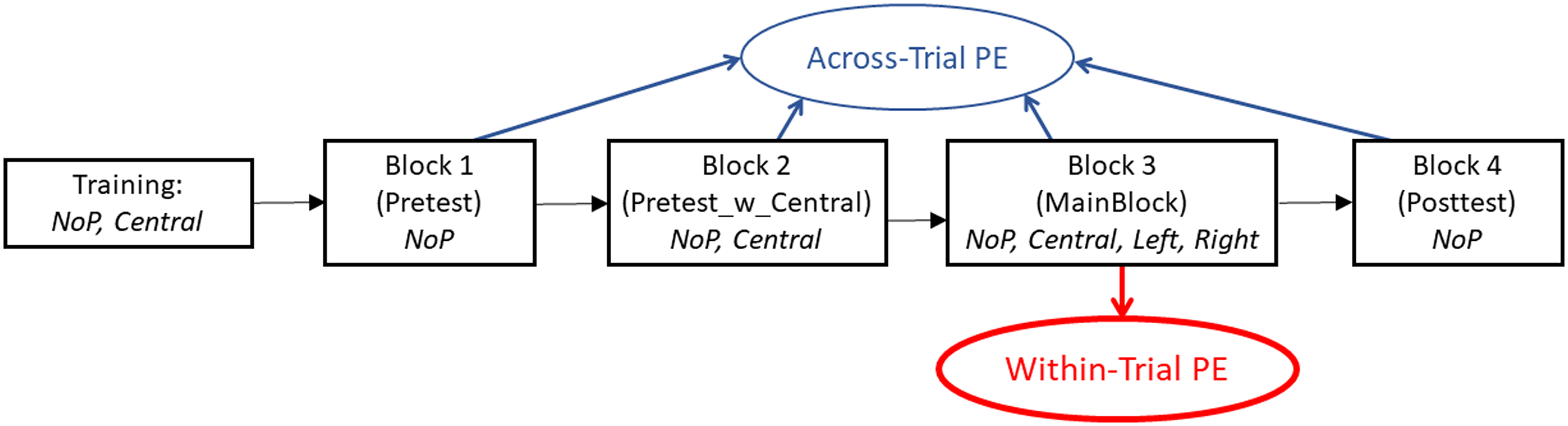
Outline of the blocks of Experiment 1. The conditions included in each block are denoted as follows: NoP = no precursor; central = central precursor; left = left-side precursor (ILD = –10 dB); right = right-side precursor (ILD = + 10 dB). The arrows indicate from which blocks the within-trial and across-trial PE are estimated.
The trials in Blocks 1, 2, and 4 were presented in completely randomized order. The trials within Block 3 were presented in pseudorandomized order. That is, the block was divided into 12 subblocks, each containing one repetition of all four P conditions combined with all T positions in completely random order (using a new randomization for each subblock and each participant). This subblocking was done to ensure a more balanced distribution of conditions across time, helping to identify any buildup of the within-trial PE. The overall duration of Experiment 1 was about 70 min (without breaks). Listeners took short breaks between the individual blocks and after completing half of the trials of the main block. Breaks between blocks were kept very short (maximally 3 min), while the break within the main block was not restricted (lasting about 5–10 min).
Modeling
The PEs observed in Experiment 1 were compared with predictions of a computational model of the auditory periphery, using the stimuli from the experiments as input signals. As the mappings of effective T ILD to perceived and to indicated azimuth (via head turn) are unknown, the model evaluation focuses on the relative shift in perceived azimuth induced by the presence of a P (i.e., the PE).
The basic modeling approach to predict the PE consists of three main components: (a) Monaural auditory frontend: For that purpose, a well-established model of the auditory periphery up to the level of the AN was used that has been shown to account for a wide variety of spectral and temporal stimulus dependencies, as measured in the AN of the anesthetized cat (Zilany & Bruce, 2006). In addition, a variant that probably provides a more realistic representation of AN spike-rate adaptation, incorporating power-law (PL) dynamics (Zilany et al., 2014; see also Zilany & Carney, 2010) was used. (b) Combination of two frontends: Left- and right-ear monaural frontends were combined to represent binaural processing. To study the impact of efferent feedback on the PE, an implementation of the MOC reflex linked to a pair of auditory frontends was used (Smalt et al., 2014). This MOC feedback mechanism dynamically controls the amount of nonlinear cochlear compression via both an ipsi- and a contralateral path. The time constants of the MOC reflex (100s of milliseconds; see Backus & Guinan, 2006) are in the order of the temporal structure of P and T stimuli used in the current study. The MOC reflex therefore potentially affects the effective ILD of T depending on the ILD of P. Smalt et al. (2014) implemented the MOC reflex by using the temporally weighted and level mapped afferent cochlear output signal at a given ear as a control signal to determine the instantaneous compression at the ipsi- and contralateral ears. To determine the impact of the MOC reflex on the PE prediction, model performance was compared between model variants with the MOC reflex turned on (NoPL_MOC_NoLSO; see Table 1 for a more complete specification of model variants) and with the MOC reflex turned off (NoPL_NoMOC_NoLSO). Smalt et al. (2014) used the Zilany and Bruce’s (2006) AN model as frontend, which incorporates exponential adaptation. To determine the potential contribution of the more realistic PL adaptation for the PE prediction, model performance was compared between two model variants without MOC reflex, one combining a pair of Zilany et al. (2014) frontends involving PL adaptation (PL_NoMOC_NoLSO) and the other involving a pair of Zilany and Bruce’s (2006) frontends (NoPL_NoMOC_NoLSO). Note that the frontend containing PL adaptation could not simply be combined with the MOC stage because the parametrization of the MOC stage in Smalt et al. (2014) was based on the frontend incorporating exponential AN adaptation. For most predictions of the current study, the output of the synapse model (i.e., without spike generator) was used as input to the next stage, the ILD extraction. Only for one model variant, which used an explicit binaural interaction stage (see below), the AN spike generator was used instead. In that case, only the Zilany et al. (2014) frontend was used, because it was found that the spike generator of the Smalt et al. model shows implausible behavior for stimulus durations exceeding 300 ms. 1 (c) ILD extraction: This stage extracts the effective (“internal”) T ILD cue in presence and absence of a P. A rectangular window was used to extract the AN response to T at the two ears. The first (and main) metric used in this study to derive the T ILD was the mean interaural spike rate difference of the windowed AN responses (referred to as ILD_AN). For the range of ILDs used in the present study (± 10 dB), this simple subtraction well represents a hemispheric-difference code for ILD (Laback et al., 2017). The second metric incorporated an explicit binaural interaction stage, namely a pair of simulated lateral superior olive (LSO) units which are known to be mainly responsible for ILD extraction (e.g., Tollin et al., 2008). For that purpose, the windowed AN responses at the two ears (Zilany et al., 2014, frontend with spike generator) were used as binaural input to both a left- and a right-side LSO model, each implementing as physiology-inspired coincidence and counting model (Ashida et al., 2017). The decision variable of this second metric corresponded to the simple difference between left- and right LSO outputs (see Klug et al., 2020), referred to as ILD_LSO (in spikes/s). To determine the impact of explicit LSO processing on the PE prediction, performance with that model variant (PL_NoMOC_LSO) was compared to the corresponding model variant based on the synapse model without the LSO stage (PL_NoMOC_NoLSO), that is, both variants incorporating PL adaptation but no MOC reflex.
Goodness of the prediction of the different model variants, in terms of RMSE and percent of variance accounted (see text).
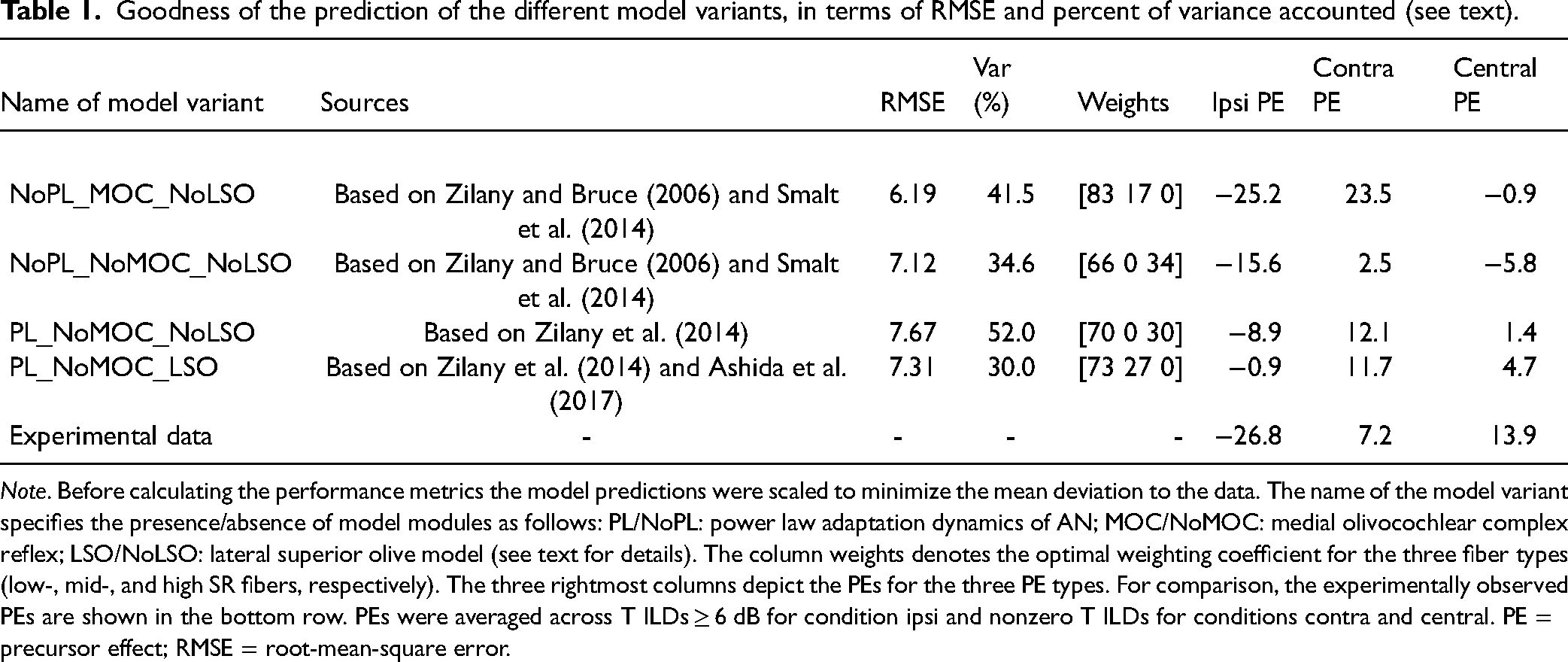
Note. Before calculating the performance metrics the model predictions were scaled to minimize the mean deviation to the data. The name of the model variant specifies the presence/absence of model modules as follows: PL/NoPL: power law adaptation dynamics of AN; MOC/NoMOC: medial olivocochlear complex reflex; LSO/NoLSO: lateral superior olive model (see text for details). The column weights denotes the optimal weighting coefficient for the three fiber types (low-, mid-, and high SR fibers, respectively). The three rightmost columns depict the PEs for the three PE types. For comparison, the experimentally observed PEs are shown in the bottom row. PEs were averaged across T ILDs ≥ 6 dB for condition ipsi and nonzero T ILDs for conditions contra and central. PE = precursor effect; RMSE = root-mean-square error.
All model variants employed standard parameters for normal hearing. A model sampling rate of 100 kHz was used. AN fibers with spontaneous rates (SRs) of 0.8, 10, and 130 spikes/s were simulated, covering the range of SRs found in cats (M. C. Liberman, 1978). For simulating the MOC reflex, the ratio of ipsi- versus contralateral pathway contributions was assumed to be 2:1 (in dB), based on physiological data approximated in Smalt et al. (2014). When using Zilany et al. (2014) as frontend, approximate implementation of PL functions and a fixed fractional noise to model the distribution of spontaneous rates were employed. The LSO parameters were taken either from Ashida et al. (2017) or from a recent study that optimized the parameters to predict ITD- and ILD thresholds (Klug et al., 2020). As in the latter study, 20 ipsilateral excitatory inputs and eight contralateral inhibitory inputs to the LSO were simulated. Predictions based on the simple AN spike rate difference metric were based on five model repetitions, each using independently generated noise stimuli. A range of CFs within + /-1 one octave around the geometric center of the T frequency band (4 kHz) were simulated, always using new random manifestations of the noise stimuli. The CF had only a small effect on the predictions. Final predictions were based on averaging of spike rates across CFs. Predictions based on the LSO-based metric were based on 30 model repetitions because of the much larger variance of that metric. For reasons of computational demand, only one CF (centered at 4 kHz) was simulated for the LSO-based metric (as was done in the model variant without LSO processing used for comparison).
The final model predictions for each model variant were obtained by weighted averaging across fiber types. Optimal weighting coefficients were determined separately for each model variant using an exhaustive search procedure that maximized the goodness of fit. The goodness of fit was quantified as the amount of explained variance. 2 Additionally, the root-mean-square (RMS) deviation between data and predictions (RMS error) was determined. As the scaling of the predictions (in spikes/s) in relation to the scaling of the data (response azimuth in degrees), both plotted on linear axes, is arbitrary, data and model predictions were normalized before determining the goodness of fit. Finally, it is worthwhile to mention that only within-trial PEs were considered in the modeling, thus, only conditions from the main block of Experiment 1 were predicted. The model was not appropriate for simulating the data from Experiment 2.
Results and Discussion
Within-Trial PE
Figure 3 shows the mean raw lateralization responses across participants (including 95% confidence intervals) from the main experimental block. The patterns of responses across conditions are reasonably symmetric across hemispheres. Given this hemispheric symmetry and for ease of interpretation, the left- and right-side P conditions were transformed into ipsilateral (ipsi) and contralateral (contra) P conditions (e.g., a left-side T combined with a right-side P represents condition contra and a left-side T combined with a left-side P represents condition ipsi). Figure 4A shows the transformed data after mirroring and averaging across sides. This hemispheric mirroring removes any overall bias and results in a completely symmetric pattern at an ILD of zero.
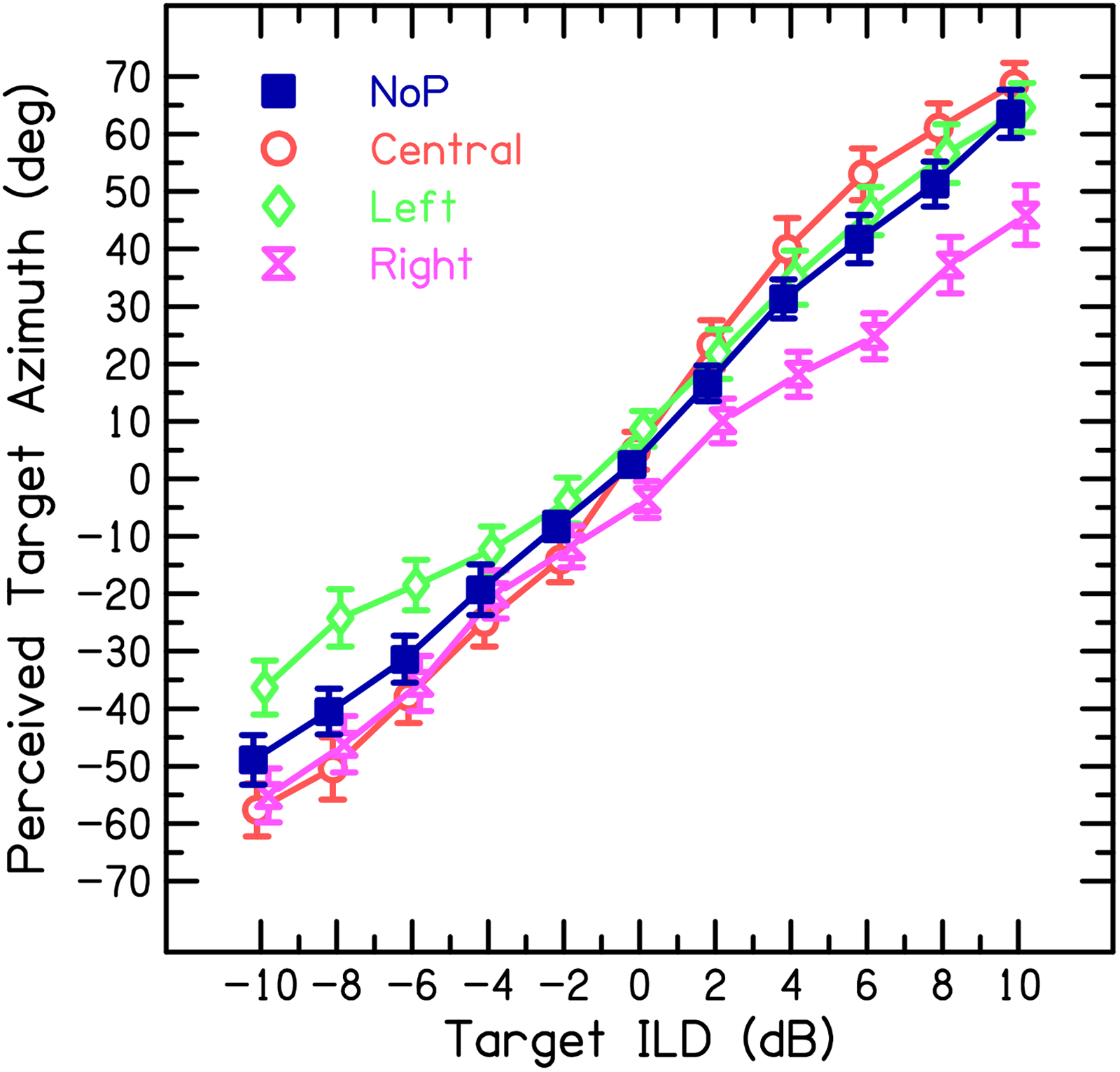
Raw results of Experiment 1, showing mean perceived azimuth of target T as a function of target ILD for five participants. Different conditions are without P (NoP), central P (Central), left-side P (Left) and right-side P (Right). Error bars indicate 95% confidence intervals. Negative ILDs indicate left-sided targets. Stimuli were band-pass-filtered noises with a center frequency of approximately 4 kHz (with 1.2- and 1-octave bandwidths of P and T, respectively).
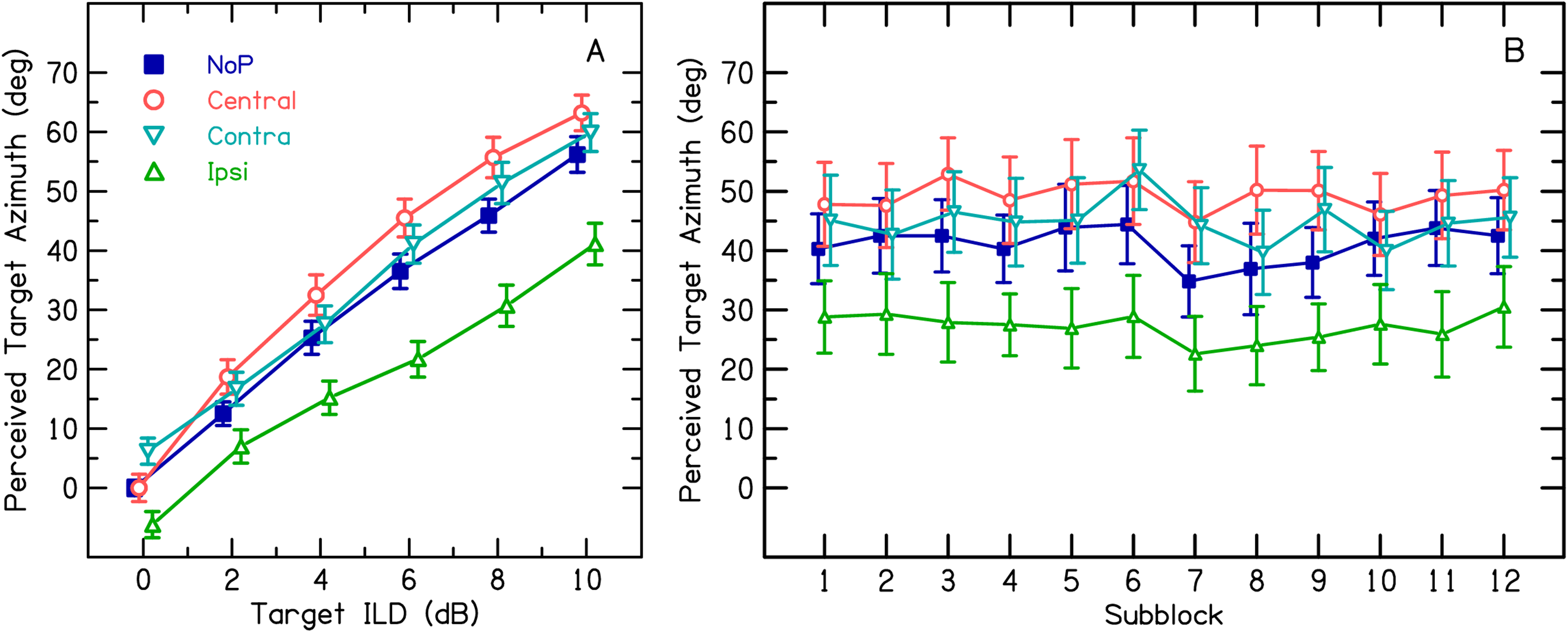
Panel A. Transformed results of Experiment 1. Data from Figure 3 were mirrored and averaged across sides and left/right precursor conditions were transformed into ipsi-/contra conditions (see text). The within-trial PEs were estimated by comparing conditions with a precursor with the NoP condition (see text). Other aspects as in Figure 3. Panel B. Time course of within-trial PEs across the subblocks of the main block (#3) in Experiment 1, based on ILDs ≥ ± 4 dB. Each subblock consisted of 44 trials, lasting about 2–3 min. Error bars indicate 95% confidence intervals.
For the reference condition without P (NoP), the perceived azimuth increases almost linearly with increasing ILD, in line with the natural azimuth versus ILD function in the tested frequency region (e.g., Blauert, 1996). The presence of Ps induced systematic shifts in perceived azimuth relative to condition NoP, that is, the PE. The PE is specified as the mean signed deviation between perceived azimuth with P compared to without P, either expressed absolutely (PE_abs; in degrees) or as proportion of the maximum perceived azimuth for condition NoP (PE_rel, in %). An ipsi P, that is, having an ILD favoring the same ear as the T ILD, shifted the perceived azimuth toward the midline. The absolute PE (in degrees) was strongest for T ILDs ≥ 6 dB (mean PE_abs: −15.1°), corresponding to a mean PE_rel of −26.8%, and decreased for smaller T ILDs. For a T ILD of zero, the perceived azimuth was shifted to the side contralateral to the P (note that the amount of this shift is exactly the same for conditions ipsi and contra because of the mirroring of data across sides). For “contralateral ILDs,” that is, when P was contralateral to T, PE_abs remained approximately constant across the entire azimuthal range of nonzero T ILDs (mean PE_abs: 4.4°), corresponding to a mean PE_rel of 7.2%. A central P shifted the perceived azimuth away from midline for all nonzero T ILDs (mean PE_abs: 7.8°; mean PE_rel: 13.9%).
The effects were supported by a repeated-measures analysis of variance (RM ANOVA) applied to the transformed lateralization data before averaging across the two sides, using the factors Target ILD, Precursor Condition, and Side. Data for an ILD of zero were excluded because the zero PE for condition central P at an ILD of zero would cause a not interpretable interaction. All the main effects were highly significant—Target ILD: F(4,160) = 587.6, p < .001; Precursor Condition: F(3,160) = 205.3, p < .001; Side: F(1,160) = 313.4, p < .001—as well as the interaction Target ILD vs. Precursor Condition—F(12,160) = 3.5, p < .001. The other two-way interactions were nonsignificant (p > .11). Tukey's post hoc test showed significant differences between all combinations of Precursor Conditions (p < .001). The interaction was found to be driven by the nonlinear lateralization function for condition ipsi: when removing condition ipsi from the ANOVA, the interaction was no longer significant (p = .87). The lack of significant interactions with the factor Side supports the hemispheric symmetry of the PE.
The results for a lateral P appear overall consistent with the previously shown medial bias for an ipsi P and sometimes even with some “bleed” across the midline, either under purely ILD- or ITD-based (e.g., Dahmen et al., 2010; Dingle et al., 2012; Kashino & Nishida, 1998; Lingner et al., 2018; Phillips et al., 2014; Phillips & Hall, 2005; Vigneault-MacLean et al., 2007) or free-field conditions (e.g., Carlile et al., 2001). Those results have mostly been explained by means of adaptation at the side of the P stimulus within the framework of hemispheric difference models (see, e.g., Vigneault-MacLean et al., 2007).
One remarkable finding of the present data is that the shift induced by a lateral P toward the contralateral side (i.e., the contra PE) persisted across the entire range of contralateral T ILDs. One potential explanation for the absence of such a complete shift in previous studies may be ceiling effects, that is, that there was not sufficient “room” for such shifts due to saturation in the lateralization function. Another potential explanation is that this effect could be specific to high-frequency ILDs, where an additional mechanism, for example, efferent compression control (see below), may come into play.
The lateral bias induced by the central P is consistent with other studies using ILD cues at low or high frequencies (Dingle et al., 2012) or low-frequency ITD cues (Kashino & Nishida, 1998; Lingner et al., 2018). This effect has been attributed to the presence of a third (midline) neural–perceptual channel, in addition to the left- and right-hemifield channels (Dingle et al., 2010, 2012) or to brainstem-specific adaptation combined with across-hemisphere comparison (Lingner et al., 2018).
Finally, Experiment 1 included a segregation cue, namely an edge pitch difference between P and T, to enhance the selective attention on T. The finding of a strong PE, despite this cue, may suggest that the PE is robust against perceptual segregation. Experiment 2 addressed this question further by selectively varying the availability of a segregation cue.
Buildup of Within-Trial PE
The within-trial effect of each P stimulus might be superimposed by an aggregate PE from preceding trials. To address the possibility of such a buildup of within-trial PEs, Figure 4B shows the mean perceived azimuths for the three P conditions and the NoP condition, calculated separately for each of the 12 subblocks of the main experimental block. Only ILDs ≥ ± 4 dB, revealing most pronounced PEs, were included for this analysis. Although there is considerable fluctuation across subblocks (note that each subblock represents only one presentation of a given condition and ILD per listener), there appears to be no systematic change across subblocks for any of the curves, suggesting no change in the amount of PE. These results were supported by a two-way RM ANOVA, including the factors Subblock and Precursor Condition. The factor Precursor Condition was highly significant—F(3,1867) = 115.6, p < .001—whereas neither the factor Subblock—F(11,1867) = 1.6, p = .09—nor the interaction—F(33,1867) = .4, p = .99—was significant. These results suggest that the time constant of any potential buildup of across-trial PE must be restricted to the duration of one subblock, which amounted to about 2–3 min. Therefore, the following modeling analysis was based on the mean PE estimate across all subblocks.
Model Predictions of Within-Trial PE
Figure 5 shows the predictions of the different model variants, each row representing a model variant. The format is similar to the experimental data plot in Figure 4A, but showing ILD_AN (in spikes/s) instead of the response azimuth on the ordinate. Results for the different fiber types (with low, mid, and high SRs) and their weighted means (for details, see below) are shown along the rows of panels. Error bars show the mean standard deviation across model repetitions. In the comparison between data and predictions, the scaling of the ordinate is somewhat arbitrary and depends on the fiber type (note also the different scale ranges on the ordinate). Performance measures for each model variant can be found in Table 1.

Model predictions of the results of Experiment 1. “Internal” ILDs (at the level of the AN or LSO, in spikes/s) are shown as a function of target ILDs. The internal ILDs are assumed to be indicative of perceived azimuth. Results for the different fiber types (with low, mid, and high SRs) and their weighted means are shown along the columns of panels (weighting coefficients for the low-, mid-, and high-SRs fibers, optimized using exhaustive search, are shown at the top of the rightmost panels). The ordinate scaling is somewhat arbitrary and depends on the fiber type. Error bars (mostly smaller than the symbols) show standard deviations across model repetitions. For each row of panels, a specific model variant was used, as specified in the lower-right corner of the leftmost panel (see Table 1 for model specification). Other aspects as in Figure 4.
We start with the model based on the Smalt et al. (2014) frontend with activated MOC feedback, as shown in the top row of panels (NoPL_MOC_NoLSO) of Figure 5. Without a P (NoP), ILD_AN increases linearly as a function of the ILD, similar to the almost linear lateralization function observed in the experimental data. The slope of the predicted function flattens from low-SR to high-SR fibers. This can be attributed to different slopes of the input/output (I/O) function (in spike rate/dB SPL) at the operation point for the different fiber types. The predicted functions for the three P types are largely parallel and show the same pattern across all three fiber types (although their slopes differ between fiber types, which again depends on the operation points along the I/O functions in presence of the particular P). While for all fiber types the relative patterns for ipsi- and contralateral Ps are qualitatively consistent with the experiment data, none of the three fiber types alone correctly predicts their relation to the interaurally symmetric conditions (NoP, central P). The rightmost panel shows predictions based on optimal weighted averaging across fiber types (i.e., 83/17/0 percent for the low-, mid-, and high-SR fibers, respectively). This “best” combination of fiber types accurately predicted the PE for condition ipsi (−25.2% vs. −26.8% observed experimentally), overestimated the size of the PE for condition contra (23.5% vs. 7.2% observed experimentally), and did not predict any central PE (−0.9% vs. 13.9% observed experimentally). Using this weighting, the model predicts 42% of the variance in the PEs (see Table 1 for performance measures). Note that while other weightings of fiber types could provide a much better prediction of the lateral bias induced by a central precursor, for example, by more emphasizing the higher-SR fibers, this would be at the price of lower predictability of ipsi and contra PEs. Thus, the optimized weighting coefficients represent a reasonable compromise. Note, however, that no conceivable weighting could explain the larger perceived azimuth for condition central P compared to condition contra P observed experimentally. Thus, the auditory periphery model is not able to predict that result. More generally, it should be mentioned that there is no commonly accepted way how the auditory system combines information from different fiber types. A conceivable argument for excluding the high-SR fibers is that at the tested stimulus level they are highly compressive and almost saturated (not shown), which makes these fibers not very sensitive to the coding of ILD cues used in the present study. Interestingly, applying a weighting of fiber types according to their prevalence as measured in the cat (16/23/61 percent; M. C. Liberman, 1978) accounts for essentially 0% of the variance in the data.
The predictions of the Smalt et al. (2014) model variant with MOC feedback deactivated (NoPL_NoMOC_NoLSO) are shown in the second row of Figure 5. For condition NoP, turning off the MOC reflex had no effect for the low-SR fibers but it flattened the predicted lateralization function for the mid-SR and even more so for the high-SR fibers (note the different scaling of the ordinate). This effect can be understood by considering the impact of compression and its control by the MOC reflex on the effective ILD (ILD_AN). With MOC reflex activated, gain from outer hair cells is reduced, resulting in a relatively steep I/O function and, consequently, also ILD_AN function. Turning off the MOC reflex increases outer hair cell activity, resulting in a flatter I/O function (and ILD_AN function) particularly for the high- and mid-SR fibers where outer hair cells may most affect the discharge rates. For the P conditions, deactivating the MOC reflex caused an overall reduction of differences between individual functions and—in case of the mid- and high-SR fibers—a flattening of functions. Although the relative pattern across P conditions is preserved, they are almost aligned with those for the NoP condition. The rightmost panel shows predictions based on optimal weighted averaging across fiber types (66/0/34 percent). Compared to the MOC reflex turned on, the predicted PEs for MOC turned off are smaller for conditions ipsi (−15.6%) and contra (2.5%) and become more negative in case of condition central P (−5.8%), together predicting 35% of the variance in the data. The reduction of predicted differences between P conditions with the MOC turned off is obviously a consequence of increased outer hair cell activity, thus indirectly demonstrating the contribution of the MOC reflex to the PE.
To study the potential role of PL dynamics in AN adaptation for the PE, the performance of the model variant including PL adaptation (PL_NoMOC_NoLSO; Zilany et al., 2014) was compared with the model variant with exponential AN adaptation (NoPL_NoMOC_NoLSO; Smalt et al., 2014), with both models having no MOC feedback. The predicted lateralization functions for variant PL_NoMOC_NoLSO (third row of Figure 5) appear to better represent the pattern of PEs than the comparison variant (NoPL_NoMOC_NoLSO). The accounted variance with optimal across-fiber weighting (0.70/0.0/0.30 percent) is clearly higher for the former variant (52% compared to 35%). This suggests that PL dynamics in AN adaptation, which was implemented in the former but not the latter model, may be responsible for the better predictability of the PEs. Interestingly, the PL_NoMOC_NoLSO model even outperforms the model variant with MOC feedback (NoPL_MOC_NoLSO) in terms of accounted variance, although these models perform quite comparably in terms of the size of predicted PEs across conditions (see Table 1).
Finally, the potential contribution of LSO processing was studied by comparing the performance of two model variants based on Zilany et al. (2014), either using the synapse model output without LSO processing (PL_NoMOC_NoLSO) or using the spike generator combined with LSO processing (PL_NoMOC_LSO). The latter model variant (bottom row of Figure 5, plotted as ILD_LSO), revealing optimal weighting coefficients of 73/27/0 percent, showed overall more variability in predictions compared to the variant based on the synapse model, as reflected by the lower explained variance of 30% (as compared to 52%). To estimate the potential contribution of the stochastic nature of the spike generator per se to the lower performance, the model variant PL_NoMOC_NoLSO was run again, but replacing the synapse with the spike generator, using the same number of repetitions as in case of model PL_NoMOC_LSO. The variability in the predictions involved by the spike generator turned out to be marginal, suggesting that the stochasticity of the spike generator per se did not significantly impact the comparison between models with and without the LSO stage. It is unclear and beyond the scope of this study to find out what aspects of LSO processing, as implemented in the coincidence and counting model by Ashida et al. (2017), and which parameter choices are critical.
In summary, the modeling results demonstrate that various aspects of PEs observed in Experiment 1 may be partly attributed to peripheral processing up to the level of the AN. It should be noted that the deliberately chosen short gap duration between P and T may have emphasized the contribution of peripheral processing. PEs measured in studies using much longer gap durations of up to 500 ms may not that easily be attributed to peripheral effects, but note that the MOC onset and decay time constants are in the order of 100s of milliseconds (see Backus & Guinan, 2006; Smalt et al., 2014). Evaluation of different model variants suggested that (a) including modeling of efferent compression reduction by the MOC reflex enhances predictability of the PEs, (b) including PL adaptation of the AN, in addition to exponential adaptation, increased predictability and resulted in best performance of all model variants, (c) including LSO processing, as implemented by the coincidence and counting model and based on previously determined parameters, results in lower predictability, and (d) none of the model variants was able to predict all types of PEs with a single set of AN fiber type weights.
Across-Trial PE
The perceived T azimuth in the NoP trials might be affected by an across-trial PE, if the time constant of the PE is longer than a trial. The subblock analysis for the NoP condition in Figure 4B showed no systematic change of perceived azimuth over time, suggesting that the time constant of a potential across-trial PE must be smaller than the subblock duration of about 2–3 min. To further evaluate a potential across-trial PE for the NoP condition, mean perceived T azimuths across the entire main experimental block (Block 3, MainBlock) was compared with the perceived T azimuths measured in the pre- and posttest (Blocks 1 and 4, respectively) that contained only NoP trials. Figure 6 shows that while pretest (cyan upward-pointing triangles) and posttest (red down-pointing triangles) perceived azimuth functions are rather similar, the function of the main experimental block (MainBlock, blue rectangles, replicated from Figure 4A) covers a smaller azimuthal range relative to the pre- and posttests. This smaller perceived azimuth range suggests an across-trial PE induced by the presence of P stimuli in the MainBlock. As the posttest block was run immediately after the main block (with a short break), the time constant of the recovery from that across-trial PE did not exceed a few minutes, that is, the duration of the break between the main block and the posttest. Figure 6 additionally shows the response function for NoP trials tested in Block 2 (Pretest_w_Central), where the NoP condition was combined with condition central P (green circles). The similarity of that response function with the corresponding pre- and posttest functions suggests that the smaller perceived azimuth range observed in condition MainBlock was caused by the lateral Ps. As the number of trials in the main block was twice as large as that of Block 2, it was also checked that restricting the analysis of the MainBlock to the first half does not change that outcome (data not shown), consistent with the subblock analysis provided above. Finally, as a sanity check the within-trial effect of central Ps in Block 2 (14.3%) was found to be very similar to the corresponding effect observed in the main block (13.9%).

Estimation of the across-trial PE. Mean-perceived T azimuth in trials without P stimuli is shown as a function of T ILD, as measured in the different blocks of Experiment 1: Pretest, Posttest, Pretest_w_Central, and Mainblock. Additionally, the dotted line shows the predicted lateralization function for the NoP trials of MainBlock, involving across-trial PE, based on weighted averaging of within-trial PEs measured in P trials of the same block (see text for details). Other aspects as in Figure 4.
To substantiate the effects, a two-way RM ANOVA was performed on the T-only trials, using the factors Test Block (Pre, Pretest_w_Central, MainBlock, and Post) and Target ILD. Both the factors Test Block—F(3,1984) = 18.2, p < .001—and Target ILD—F(5, 1984) = 11.0, p < .001—as well as their interaction—F(15,1984) = 2.4, p < .002—were highly significant. A post hoc test on the factor Test Block revealed that condition MainBlock differed significantly from all other conditions (p < .001), while the other three conditions did not differ significantly from each other (p ≥ .275 for all). A control RM-ANOVA, restricting the data from MainBlock to the first half, resulted in similar main effects and interaction, with slightly larger p-values for the post hoc differences between MainBlock and the other conditions (< .001, .002, .014 for conditions Pre, Pretest_w_Central, and Post, respectively). The differences between the latter three conditions did not change (p > .269 for all).
The effective reduction of perceived azimuth range in condition NoP of the main block compared to the pre- or posttests (i.e., the across-trial PE) appears to be reminiscent of the previously shown role of the spatial distribution within a preceding sound (Dahmen et al., 2010; Gleiss et al., 2019) or across a sequence of preceding sounds (Hládek et al., 2017; Kopčo et al., 2007). Increasing the variance of the ILD-distribution of an adapter stimulus with dynamically varying ILD was shown to flatten the left/right discrimination function and to increase the ILD threshold for a subsequently presented static test stimulus (Dahmen et al., 2010). In the current study, P ILDs were always static within a stimulus (P or T) but varied across trials. Hládek et al. (2017) demonstrated contextual localization effects over time scales far exceeding a single trial (in the order of minutes), thus, across-trial effects of the ILD distribution may also have impacted the current results. In our pre- and posttests (without Ps) the distribution was rectangular, whereas in the main block (with Ps) it was multimodal with peaks at −10, 0, and + 10 dB. Mathematically, the “peaky” distribution of the main block has a slightly larger variance (standard deviation: 7.2 dB) than the flat distribution of the pre- and posttests (standard deviation: 6.4 dB), thus, the reduction in perceived azimuth range in the main block appears consistent with the increase of the distribution's variance. However, particular aspects of the ILD distributions that are not well captured by the variance measure may be important. Based on the observed within-trial PEs, distribution peaks at + /–10 dB are expected to, on the one hand, reduce the perceived azimuth (i.e., causing a medial bias) due to the ipsi PE and, on the other hand, to increase the perceived azimuth (i.e., causing a lateral bias) due to the contra PE. Additionally, the distribution peak at 0 dB is expected to cause a lateral bias (due to the central PE). To find out if combining these observed within-trial PEs (in degrees) can predict the observed across-trial PE, their weighted average was determined and used to alter the reference lateralization function (mean of pre- and posttest functions) and to compare the outcome to the function from the main block. When using equal weights for the three P types, essentially no across-trial PE is predicted; thus, the medial and lateral biases seem to cancel each other out. Then, the relative weights of the three potential sources of bias were allowed to freely vary to find the lateralization function that showed the smallest rms deviation, across T ILDs, from the lateralization function measured in the MainBlock. The target ILD of zero was excluded from the weight optimization, because for a midline T in a symmetric arrangement a lateralization bias should not occur (and indeed was not observed) because any across-trial medial and lateral biases should cancel each other out on average across all trials. For the optimal weights (70/16/14 percent), the predicted lateralization function (dotted line in Figure 6) well aligned with the lateralization function from the main block (RMSE = 1.16 degrees). In other words, the medial bias in the T lateralization function in NoP trials of the MainBlock (i.e., the across-trial PE) could be well predicted by the accumulated within-trial PEs in P trials, when assuming a dominating contribution of ipsi Ps and low contributions of contra and central Ps.
Experiment 2: Role of Perceptual Segregation
A recent model of the PE, proposed by Lingner et al. (2018), assumes that the PE mechanism operates directly upon the within-channel localization information extracted in the brainstem. Therefore, this model implicitly assumes that the mechanism is independent of perceptual grouping which is often assumed to take place at higher processing stages (e.g., Cusack, 2005). This assumption of independence of the PE of perceptual segregation seems to be, however, not experimentally verified. Previous PE studies typically used the same stimulus as T and P. This may have promoted perceptual fusion and therefore have provided a restricted view on the PE, if the PE is indeed affected by sequential segregation. Experiment 1, on the other hand, included a spectral difference between P and T to promote segregation. Kopčo et al. (2017) and Hládek et al. (2017) reported some hints for a role of perceptual similarity between context and T stimuli, but a reduction of PE (“contextual bias” in their nomenclature) was observed mainly in configurations causing “attractive” bias, that is, a shift of perceived azimuth toward the P, which was not observed at all under the conditions of the present study.
Experiment 2 addressed the potential role of precursor-target segregation in the PE by introducing a pitch difference, which is known to be a very efficient segregation cue (e.g., Carlyon, 2004; B. C. J. Moore & Gockel, 2012) and avoids some of the abovementioned potential confounds of changing the P duration. There are three main scenarios regarding the potential effect of such a segregation cue. Scenario 1 assumes that the PE is directly modulated by perceptual grouping, in which case one would expect a smaller or even absent PE in case of a segregation cue that perceptually separates P and T, as compared to without such a cue. Such an influence could operate by means of a top-down control path, directly modulating the PE (one possibility would be via central control of the MOC reflex). This scenario, thus, assumes the importance of the perceptual similarity of P and T stimuli in the PE (Hládek et al., 2017; Kopčo et al., 2017). The observation of PEs in Experiment 1, despite the presence of a segregation cue, an edge pitch difference, may already argue against this scenario. However, in theory the PE could be even stronger without segregation cue. Scenario 2 assumes that the PE mechanism is completely independent of auditory grouping, as explicitly or implicitly assumed in several PE studies (e.g., Lingner et al., 2018; Maier et al., 2010). If it is further assumed that the segregation cue itself does not impact the perceived azimuth, no effect of the presence of a segregation cue (on the amount of PE) is expected in this scenario. Scenario 3, a variant of Scenario 2, also assumes that the PE is entirely independent of auditory grouping, but that the stimulus change required to induce the segregation cue per se affects the perceived azimuth in a way that modifies the PE. Alternatively, the stimulus change might affect the ability to segregate P and T independent of the PE, for example, by means of modulating attentional focus. All these effects could change the PE in both directions, causing either a reduction or an increase. Taken together, the only unambiguous outcomes would be an increase of the PE (Scenario 3) or no PE change at all (Scenario 2), whereas a decrease of the PE would be compatible with both Scenarios 1 and 3. As it was a priori unclear if the envelope rate of either T or P should better be varied, Experiment 2A varied the rate of T and kept P constant, and Experiment 2B varied the rate of P and kept T constant.
Experiment 2A
Methods
Given the dependence of the PE on the spectral overlap of P and T (e.g., Kashino & Nishida, 1998; Phillips & Hall, 2005), it was important to introduce a segregation cue that does not alter the stimulus’ spectral range. A suitable solution for that purpose appeared to be a temporal pitch difference between P and T, using so-called transposed-noise stimuli (van de Par & Kohlrausch, 1997) having different temporal envelope rates and being filtered in the same frequency region. Thus, in the condition promoting sequential grouping (No-PitchCue), P and T stimuli had the same envelope rate (125 Hz), whereas in the condition promoting sequential segregation (PitchCue) the T had the double envelope rate (250 Hz) of the P. Such an octave difference in temporal pitch approximates the fundamental frequency difference between male and female voices, thus producing a rather salient pitch difference.
The transposed-noise stimuli were generated by band-pass-filtering Gaussian white noise at a center frequency of either 125 or 250 Hz (sixth-order Butterworth filter with 3-dB bandwidth of 25 Hz), extracting the envelope signal by half-wave rectification and low-pass-filtering at 2000 Hz (12th-order Butterworth filter) and subsequently modulating a 4-kHz pure tone with that envelope signal. The choice of the parameters was guided by the additional requirement that the same stimuli should provide salient envelope ITD cues (Bernstein & Trahiotis, 2003), which were used for the purpose of another study.
The PitchCue and No-PitchCue conditions were each tested in all four P configurations (like in Experiment 1). Two blocks with the PitchCue condition and two blocks with the No-PitchCue condition were tested in counterbalanced order across participants. Each block included six repetitions of each of the 11 T ILDs for each P condition, resulting in 264 trials per block. The P and T ILDs, as well as all other aspects of the experiment (including the listeners), were the same as in Experiment 1. Listeners took breaks of about 5 min between the individual blocks.
Results and Discussion
The overall pattern of results for the different P conditions appears at first sight relatively similar across the two stimulus conditions PitchCue and No-PitchCue (shown in the upper left and right panels of Figure 7, respectively), but there were also some systematic differences. For ease of comparison, the left panel of Figure 8 compares the corresponding unsigned PEs, averaged across nonzero T ILDs, between the PitchCue (white bars) and No-PitchCue (black bars) conditions. In case of central and contra Ps, the PE tends to be slightly smaller for the PitchCue condition (mean difference between conditions No-PitchCue and PitchCue for nonzero T ILDs: 5.0 and 4.5 degrees, respectively). In case of the ipsilateral P, however, the PE is clearly larger for the PitchCue condition (mean difference: 10.0 degrees). This clearly larger ipsilateral PE in the PitchCue condition appears to be due to two effects in the lateralization functions (see Figure 7): in the PitchCue condition, the overall amount of lateralization was, first, larger with T alone (condition NoP) and, second, smaller with the ipsilateral P (condition ipsi), as compared to the No-PitchCue condition.

Results of Experiment 2 testing the effect of introducing a pitch difference between precursor and target stimuli. Stimuli were transposed noises with envelope rates for target and precursor as specified in each panel (see text for details). The upper panels show results from part A of the experiment: the PitchCue condition (left panel) has a higher target envelope rate (denoted in the panels) than the No-PitchCue condition (right panel), whereas the precursor rate is the same. The lower panels show results from part B of the experiment: the PitchCue and the No-PitchCue conditions have the same target envelope rate, whereas the precursor envelope rate is higher in the No-PitchCue condition than in the PitchCue condition. Other aspects as in Figure 4.

Mean unsigned PEs (in %) estimated from the data in Figure 7 (see text for details). Data from part A are shown in the left panel, and data from part B in the right panel. The PitchCue conditions are indicated with white bars and the No-PitchCue conditions with black bars. The statistical significance of the difference with/without pitch difference is indicated above the bars: n.s. = not significant, * = p ≤ .05, ** = p ≤ .01. Error bars indicate standard deviations.
A three-way RM-ANOVA was conducted using the factors Pitch Cue Presence, Target ILD, and Precursor Condition. All main effects were significant—Pitch Cue Presence: F(1,160) = 5.8, p = .016; Target ILD: F(4,160) = 1311.9, p < .001; Precursor Condition: F(3,160) = 200.5, p < .001—as well as the interactions Pitch Cue x Precursor Condition—F(3,160) = 7.6, p < .001—and Pitch Cue Presence x Precursor Condition x Target ILD—F(28,160) = 1.7, p = .009. The significant three-way interaction indicates that the pitch cue affected the PEs. Given this interaction, the two pitch cue conditions were also analyzed separately. For condition PitchCue, a two-way RM-ANOVA with the factors Target ILD and Precursor Condition showed significant effects of both factors—Target ILD: F(4,160) = 704.5, p < .001; Precursor Condition: F(3,160) = 143.2, p < .001—and of their interaction—F(12,160) = 2.1, p < .017. A Tukey's post hoc test (using the 5% significance criterion) showed significant differences between all combinations of P conditions except between NoP and contra. Thus, with the pitch cue, the contralateral P had no effect. The analog RM-ANOVA for condition No-PitchCue showed the same overall outcome—Target ILD: F(4,160) = 643.8, p < .001; Precursor Condition: F(3,160) = 71.4, p < .001; interaction: F(12,160) = 1.9, p < .029. However, in this case the post hoc test showed significant differences between all combinations of P conditions.
To find out which of the PEs were affected by the pitch cue, separate RM-ANOVAs were performed for each of the three Precursor Conditions, each paired with condition NoP, and evaluating the interaction Pitch Cue Presence x Precursor Condition. Thus, this analysis evaluated the significance of the effects of the pitch cue shown in Figure 8 (marked with asterisks). The interaction was nonsignificant for the pairs central/NoP (p = .071) and contra/NoP (p = .066), but highly significant for the pair ipsi/NoP (p ≤ .001). Finally, two RM-ANOVAs were conducted to evaluate the effect of the presence of a pitch cue on the perceived azimuth for two particular conditions; for condition NoP, there were significant main effects—Pitch Cue Presence: F(1,40) = 18.2, p < .001; Target ILD: F(4,4) = 373.6, p < .001—but no interaction—F(4,40) = 0.53, p = .71; similarly, for condition ipsi, there were significant main effects—Pitch Cue Presence: F(1,40) = 7.0, p = .008; Target ILD: F(4,40) = 309.0, p < .001—but no interaction—F(4,40) = 1.0, p = .383).
To summarize, the presence of a pitch cue caused a larger PE for ipsilateral Ps but had no significant effect for central and contra Ps, as compared to without a pitch cue. Furthermore, the pitch cue caused an overall larger perceived azimuth for NoP trials. This stronger T lateralization in the PitchCue condition was initially not anticipated, but it was soon realized that this effect could be an effect of the higher T envelope rate (250 Hz) as compared to the No-PitchCue condition (125 Hz). Increasing the stimulus envelope rate from 100 to 400 Hz has been shown to improve ILD thresholds (Laback et al., 2017) and increasing the stimulation pulse rate has been shown to increase extent of perceived stimulus laterality (azimuth) in electric hearing with cochlear implants (CIs) (Anderson et al., 2019). 3 Importantly, increased perceived azimuth with higher envelope rate should not directly affect the estimated PE because it affects all conditions (with and without Ps) by the same amount. Nevertheless, in case of the ipsilateral P the presence of the pitch cue resulted in reduced perceived azimuth, suggesting that for that condition some mechanism counteracted and dominated the T-envelope-rate based increase of perceived azimuth.
The outcome for the ipsi P appears to be most compatible with Scenario 3, according to which the PE mechanism is independent of auditory grouping. What mechanism(s) could have caused the larger ipsi PE in presence of a pitch cue, if grouping effects would predict the opposite effect? One possibility could be that the higher T envelope rate increased the efficiency of the ipsi P as a consequence of some type of across-trial (long-term) PE (Dahmen et al., 2010; Experiment 1 of the present study). Assuming that the higher T envelope rate widened the “effective” long-term ILD distribution, the resulting narrowing of auditory space (Dahmen et al., 2010) might have interacted with the within-trial ipsi PE, particularly to reduce the overall perceived azimuth in that condition.
Another explanation could be that the pitch cue modified the ability to segregate P and T independent of the PE, for example, by means of modulating the attentional focus on T. According to this explanation, without a segregation cue T lateralization is biased toward P because more binaural information of P “leaks” into the mental representation of T (i.e., reducing the relative contribution of the PE on T). Such a grouping effect has been proposed to explain a reduction of “attractive” PE (Hládek et al., 2017; Kopčo et al., 2017). Applying such an explanation to the present data, with a segregation cue the perceived azimuth should shift away from P, which means toward midline for the ipsi (which is consistent with the data) and toward the side for central and contra P conditions (which is consistent with the higher absolute perceived azimuth for those conditions, although not with the nonsignificant change in PE).
Taken together, the pattern of results of Experiment 2A appears to support the conclusion that the PE per se is not modulated by sequential segregation. In more detail, the observed effects of the pitch cue might be explainable by within-trial as well as across-trial effects of the T envelope rate and by higher order attentional effects.
Experiment 2B
Motivation and Methods
In Experiment 2A the envelope rate (and, thus, the pitch) of the P stimulus was kept constant (at 125 Hz), which had the advantage of avoiding any direct effects of the P envelope rate on the PE. On the other hand, the T envelope rate was varied (either 125 or 250 Hz), resulting in an overall larger perceived azimuth in the condition with the higher rate, that is, condition PitchCue. While it was argued that this increased perceived azimuth should have affected all conditions by the same amount, thus not affecting the estimated PE, it was also noted that other effects like medial bias due to across-trial effects of envelope rate changes or higher order attentional effects could be involved.
Therefore, to obtain a more complete picture, a control experiment was conducted in which the T envelope rate was kept constant at 250 Hz and the P envelope rate was either 125 Hz (PitchCue condition) or 250 Hz (No-PitchCue condition). The T was fixed at the higher rate based on informal pretests, suggesting that in case of unmatched rates of T and P, listeners find it easier to focus on a T with a higher rather than with a lower rate.
The experiment was conducted about 6 months after completing Experiment 2A. A total of five listeners completed the experiment. Three of them already participated in Experiments 1 and 2A, and two of them were new, replacing two listeners from the earlier experiments who were no longer available. The new listeners fulfilled the same inclusion criteria (see Methods of Experiment 1). All other aspects of the experiment were the same as in Experiment 2A.
Results and Discussion
The lower panels of Figure 7 show the results of Experiment 2B, in the same format as in Experiment 2A, with the left panel plotting the PitchCue condition and the right panel plotting the No-PitchCue condition. The effects of the pitch cue are summarized in the right panel of Figure 8, showing the mean PEs with and without pitch cue for the three P conditions. The overall pattern of PEs appears quite similar to Experiment 2A, with the most apparent effect being a stronger ipsi PE in presence of the pitch cue. Besides, the presence of the pitch cue tends to decrease the central PE and, probably, also the contra PE.
The statistical analysis was conducted analog to Experiment 2A. A three-way RM-ANOVA showed significant main effects of all three factors—Pitch Cue Presence: F(1,160) = 27.0, p = .001; Target ILD: F(4,160) = 1135.8, p < .001; Precursor Condition: F(3,160) = 251.6, p < .001—as well as the interactions Pitch Cue Presence x Precursor Condition—F(3,160) = 7.9, p < .001—and Pitch Cue Presence x Precursor Condition x Target ILD—F(28,160) = 4.2, p = .001. As in Experiment 2A, the significant three-way interaction indicates an effect of the pitch cue on the PEs. Given this interaction, the two pitch cue conditions were also analyzed separately. The two-way RM-ANOVA for the PitchCue condition showed highly significant main effects—Target ILD: F(4,160) = 615.8, p < .001; Precursor Condition: F(3,160) = 160.6, p < .001—and their interaction—F(12,160) = 5.0, p < .001. A post hoc test showed significant differences between all combinations of P conditions except between central and contra. For the No-PitchCue condition, the corresponding RM-ANOVA showed the same pattern of significant main effects—Target ILD: F(4,160) = 529.3, p < .001, Precursor Condition: F(3,160) = 101.5, p < .001; their interaction: F(12,160) = 4.4, p < .001—and the post hoc test on Precursor Conditions.
For direct comparison across the pitch cue conditions, separate RM-ANOVAs were performed for each of the three P conditions, each paired with condition NoP, and the interaction Pitch Cue Presence vs. Precursor Condition was evaluated. The interaction was highly significant for the pairs central/NoP (p = .009) and ipsi/NoP (p ≤ .001) but not for the pair contra/NoP (p = .132). Finally, two RM-ANOVAs were conducted to evaluate the effect of the pitch cue on the perceived azimuth for two particular conditions; for condition NoP, there were significant main effects—Pitch Cue Presence: F(1,40) = 43.6, p < .001; Target ILD: F(4,4) = 304.6, p < .001—and a significant interaction—F(4,40) = 3.8, p = .004. For condition ipsi, there was no significant main effect of Pitch Cue Presence—F(1,40) = 1.0, p = .317; a significant effect of Target ILD—F(4,40) = 187.3, p < .001; and no interaction—F(4,40) = 1.1, p = .346.
Overall, the statistical analysis is consistent with the main observation from Experiment 2A that the presence of a pitch cue significantly increased the ipsi PE. In contrast to Experiment 2A, however, it shows that the presence of the pitch cue significantly reduced the central PE. As for Experiment 2A, the lateralization functions of the individual conditions were inspected more closely.
The significantly larger perceived azimuth in NoP trials in presence of the pitch cue cannot be attributed to the T envelope rate, like in Experiment 2A because here it was held constant at 250 Hz. Rather, this effect might be attributed to the narrower “effective” across-trial ILD distribution as a result of the lower P rate, which could widen auditory space. However, to predict the observed increase of ipsi and the decrease of central/contra PEs (though the latter was not significant), this widening of auditory space needs to be assumed to have less impact on NoP compared to P conditions. One potential explanation could be that the perceived azimuth in NoP trials was more influenced by a widening of auditory space due to across-trial PE than the perceived azimuth in P conditions where the within-trial PE dominated.
Assuming the involvement of modulation in attentional focus, analog to Experiment 2A, improved sequential segregation by means of the pitch cue would shift the perceived azimuth away from P, thus, toward midline for the ipsi and toward the side for central and contra conditions. This effect alone could, thus, explain the increase in ipsi PE but it would not explain the decrease in central PE.
In summary, introducing a pitch cue by changing the P envelope rate produced an overall similar change in the pattern of PEs as by changing the T envelope rate in experiment 2A. In both cases the presence of a pitch cue was shown to increase the ipsilateral PE (i.e., the strongest type of PE), which supports the interpretation that the ipsilateral PE is independent of auditory grouping (Scenario 3). In experiment 2B the central PE decreased significantly in presence of the pitch cue (consistent with both Scenarios 1 and 3), while in Experiment 2A it did not change significantly. The contra PE did not change significantly by the presence of the pitch cue, consistent with Experiment 2A. Combining Experiments 2A and 2B, the effects of a pitch cue appear to be more consistent with within-trial and across-trial effects of envelope rate changes of P and T stimuli and attentional effects, rather than with auditory grouping mechanisms modulating the PE.
As a final sanity check, a direct comparison between the PitchCue conditions of Experiments 2A and B, both employing the same stimuli, reveals an overall smaller response range in the latter case (Figure 7). This turned out to be mainly due the replacement of two of the five participants who exploited the response range to a lesser extent. Still, this demonstrates that the absolute range of lateralization can considerably differ between separate blocks of trials. Importantly, the relative patterns across conditions are very similar between Experiments 2A and 2B (Figure 8) and all the analyses described above involved only within-experiment comparisons.
General Discussion
This study investigated the properties and mechanisms involved in contextual lateralization based on ILDs. A head-pointing paradigm was used to measure the perceived azimuth of a target (T) stimulus, using high-frequency stimuli presented via headphones. The first main goal was to characterize the effects of the presence and lateral position of a precursor (P) stimulus on the perceived azimuth (Experiment 1). The second main goal was to gain insight into the peripheral mechanisms contributing to the ILD-based PE, with the help of a model of the auditory periphery. The third main goal was to study the role of perceptual segregation of P and T for the PE (Experiment 2).
The subject pool tested was quite limited (five listeners per experiment). Although the results were sufficiently consistent across listeners to draw overall conclusions, future studies should study more subjects to better estimate the variability of effects across the normal-hearing population. Before discussing various aspects of the results, it is worthwhile to evaluate the general validity of the experimental paradigm used. To approximate the situation of relatively fast switching between sound sources in multisource environments, a short gap between P and T (10 ms) was chosen, and listeners were instructed to focus on T and ignore P. An important question is if the listeners managed to selectively focus on T. Had listeners just integrated binaural information of P and T, responses would be expected to be biased toward P. In fact, the observed response bias (i.e., the PE) was found to be always in the direction away from P (i.e., repulsive). This indicates that listeners were able to efficiently “window” the PE-adapted T information, although this does not exclude some leakage of P information into the presumably sluggish binaural temporal window applied on T (e.g., Kolarik & Culling, 2009), which is assumed to occur after the PE mechanism (see below). In the subsections that follow the findings regarding the three main goals are put into wider context and, finally, the implications for spatial hearing in real-life situations are outlined.
Within-Trial Versus Across-Trial PE
Contextual localization/lateralization of a T stimulus following a sequence of more than one P stimuli involves both a short-term (within-trial) component, that is, the effect of the immediately preceding P, and an across-trial component, that is, the effect of the “history” of Ps. In the present Experiment 1, the strategy to determine the within-trial PE (10-ms silent gap and 610-ms onset delay between P and T) for a range of P conditions was to compare responses from trials containing a P to those from trials without a P, with all these trials being randomly interleaved in one big block. The within-trial PE was then quantified as the difference in perceived azimuth obtained in trials with a P compared to trials without a P, expressed as percentage of the lateral response range.
The general patterns of within-trial PEs estimated for the three P types (ipsilateral, contralateral, and central), showing lateral bias for central Ps and considerable medial bias for ipsilateral Ps (amounting to 27% of the response range), were found to be overall consistent with previous studies, using either ILD or ITD as binaural cues (Dahmen et al., 2010; Dingle et al., 2012; Kashino & Nishida, 1998; Lingner et al., 2018; Phillips et al., 2014; Phillips & Hall, 2005; Vigneault-MacLean et al., 2007). The effect of a lateral P was shown to extend to the contralateral side, causing a slight lateral bias for targets across the entire contralateral hemisphere (see Figure 4A), and appears to be specific to high-frequency ILDs as this has not been reported for low-frequency ITDs (see particularly data of Lingner et al., 2018, who used a similar paradigm).
A follow-up analysis on the data of Experiment 1 checked for potential temporal dynamics of the within-trial PEs over the course of the experiment. The results showed no evidence for a buildup of the within-trial PE across the 12 subblocks of the main experimental block. Given the duration of about 2–3 min of each subblock, this suggests that if a buildup of within-trial PEs exists, it must be shorter than this duration.
Experiment 1 showed evidence, though, for an across-trial PE in trials without P (NoP condition). The overall range of perceived T azimuths of NoP trials from the main block, which were randomly interleaved with trials containing Ps, was about 18% smaller compared to the perceived T azimuths obtained in separate blocks without Ps that were measured before and after the main block (pre- and posttests, respectively). As there was no transfer of the across-trial PE from the main block to the posttest, between which there was only a very short break, the time constant of this across-trial PE must be quite restricted, ranging from a few minutes on the upper end to the interval between subsequent trial on the lower end. Such a restricted time constant is consistent with the reported lack of a change in perceived target azimuth in NoP trials across the course of experimental block.
Previous studies have shown that the ILD statistics of preceding stimuli systematically impact auditory spatial perception (Dahmen et al., 2010; Gleiss et al., 2019). Particularly, they showed that the mean of the P's ILD distribution biases the perceived azimuth, whereas its variance affects the slope of the lateralization function (which is supposed to determine spatial sensitivity). These studies varied the ILD distributions on a quite short time scale (within about one second), while a study on contextual localization suggested buildup times in the order of minutes (Hládek et al., 2017). Combining these insights from previous studies, the observed across-trial PE might be understood in terms of the shape of the across-trial ILD distribution in the main block compared to the pre- and posttest blocks. Notably, the presence of Ps in the main block did not increase the width of the across-trial ILD distribution and only slightly increased the distribution's variance compared to the pre- and posttests. It was found that the overall reduction of perceived azimuth by the presence of P stimuli can be predicted by weighted averaging of within-trial PEs when assuming dominance of the medial bias by ipsi Ps over lateral bias by contra and central Ps. Thus, the across-trial PE might be understood as an across-trial accumulation of within-trial PEs. However, future work is required to provide direct support for such an interpretation.
Finally, given the above results, one may wonder if the lateral bias induced by the central P was really a within-trial effect, or if it was just a consequence of an interaction of across-trial and within-trial PEs, resulting in smaller perceived azimuth for the NoP than for the central P condition. If this were the case then in Block 2 of Experiment 1, containing only conditions NoP and central P, no central PE (i.e., lateral bias) would be expected at all. In fact, the central PE was very similar in size whether measured in Block 2 (not shown, 14.3%) or in the main block (13.9%), indicating that it is a “real” within-trial PE. Interestingly, in Block 2 no lateral bias was observed for condition NoP (compared to the pre- and posttests), as might be expected by the presence of central Ps in the same block. This seems to be consistent with the assumption of a general dominance of the ipsi PE.
Insights on Mechanisms Underlying the Within-Trial PE Based on Modeling
The overall similarity in PEs for ILDs and ITDs (e.g., Phillips & Hall, 2005) might at first sight indicate that PEs arise entirely at the level of first binaural interaction, namely the LSO for ILDs (Magnusson et al., 2008) and the medial superior olive for low-frequency ITDs (Stange et al., 2013). However, in the current study it was conjectured that ILD-based PEs might at least partly already be shaped in the auditory periphery. To that end, the results of Experiment 1 were predicted by different variants of a model of the auditory periphery up to the level of the AN (incorporating the MOC reflex). The effective (“internal”) T ILD at the level of the AN (ILD_AN) was quantified as the mean interaural spike rate difference (Laback et al., 2017). Best predictions were obtained by model variants that contained either realistic AN adaptation (Zilany & Carney, 2010) or binaurally linked compression control characteristic of efferent (MOC-based) feedback (Smalt et al., 2014). Overall, the modeling outcomes show that already the auditory periphery significantly shapes the internal presentation of T ILDs, with and without Ps, in a way that partially predicts the behaviorally observed PEs. While PE models presented so far were either rather abstract (e.g., Dingle et al., 2010, 2012) or focused on processing stages beyond the AN (Lingner et al., 2018), the present results suggest that future more complete attempts to model the ILD-based PE would benefit from incorporating the nonlinear transformation of external ILDs in the auditory periphery.
With appropriate model configurations, both model variants qualitatively predicted the medial bias by an ipsilateral P and the lateral bias by a contralateral P. The lateral bias by a central P was not or only marginally predicted when optimizing the relative weighting of individual AN-fiber types for the entire data set. However, individual fibers, particularly the high-SR fibers, could predict that effect. Surprisingly, weighting of fiber types according to their prevalence in the cat (M. C. Liberman, 1978) provided rather poor predictions. It is currently not clear how the human central auditory system selects and combines relevant fiber types at a given stimulus level, which represents a general open issue in predicting auditory effects based on firing rates.
Different model configurations were tested, attempting to deduce the contribution of mainly two mechanisms to the PE. First, the role of AN adaptation, and particularly of PL dynamics that was shown to account for dynamic range adaptation (Zilany & Carney, 2010) and is therefore a candidate mechanism for explaining adaptive effects in ILD-based sound lateralization (Dahmen et al., 2010; Gleiss et al., 2019), was studied by predicting the model performance for the following two model variants without MOC feedback: the Smalt et al. (2014) model that incorporates short-term exponential adaptation (Zilany & Bruce, 2006) and the Zilany et al.’s (2014) model that additionally incorporates PL dynamics with a longer time constant. The better prediction power of the latter model seems to indicate that PL dynamics of the AN contributes to the PE. One caveat is that some other differences between the Zilany et al.’s (2014) and the Zilany and Bruce’s (2006) frontends, besides PL adaptation, may have influenced their comparison.
Second, the particular contribution of efferent cochlear compression control by the MOC reflex was studied by comparing the performance of the Smalt et al., 2014 model with MOC feedback either turned on or off. The higher prediction power for the former (42%) compared to the latter variant (35%) suggests that MOC-like compression control indeed contributes to the PE. For condition NoP activation of the MOC reflex was shown to steepen the predicted lateralization functions, thus partly undoing the compression of ILDs, particularly for mid- and high-SR fibers. For the P conditions it caused overall increased effects of ipsi- and contralateral Ps which better reflected the experimental data than the model variant with MOC turned off. On a more detailed level, the results of Experiment 1 showed that the lateral bias caused by contralateral Ps persisted across the entire contralateral hemifield and this effect was predicted by the model variant that includes MOC feedback. Thus, the MOC (but also PL adaptation) might contribute to this specificity of the ILD-based PE.
The potential contribution of the MOC reflex suggested by the current modeling of ILD-based PEs is interesting in the light of a recent histological study in humans (L. D. Liberman & Liberman, 2019), showing that the prevalence of cochlear projections of MOC fibers is highest in the mid-to-high frequency region that typically conveys most salient ILD cues. The time constants of the MOC, as implemented in the Smalt et al. (2014) model (based on Backus & Guinan, 2006), are in the order of a few dozens to a few hundreds of milliseconds, thus well matching the time constants of the within-trial PEs studied here. On the other hand, the time constants of PL adaptation also fall into this range. For future studies it would be interesting to explore the ability of models including MOC, PL adaptation or even their combination to predict PEs for various temporal configurations of P and T, possibly even including the across-trial PE.
On a more general level, the overall similarity between current within-trial ILD-based PEs and ITD-based PEs reported in the literature may appear to undermine the roles of AN adaptation and the MOC reflex to some extent. However, in more detail, the situation could be more complex. First, it is possible that AN adaptation and the MOC particularly enhance ILD-based PEs, in addition to other mechanisms that operate independent of the particular binaural cue, like adaptation in early binaural interaction (e.g., Magnusson et al., 2008). Direct comparison of ILD- and ITD-based PEs in one experiment would be required to evaluate the relative strengths of ILD- and ITD-specific effects. Second, it is possible that at least the MOC contributes also to the ITD-based PE, for example, by introducing interaural delays as a consequence of changes in the impulse response of auditory filters when outer hair cell gain is changed.
Finally, it was tested whether replacing the simple ILD_AN metric by a more physiology-based ILD extraction stage, based on the relative outputs of simulated left- and a right-ear LSOs, may further enhance the prediction power of the PL adaptation model. However, including an LSO-stage, based on the coincidence and counting model by Ashida et al. (2017), actually reduced the prediction power. It should be noted, though, that this quite focused modeling approach was based on a multitude of fixed parameter settings that had been optimized in previous studies based on different data. To obtain a more complete view, more extensive future modeling should systematically explore the effects of the most critical model parameters as well as their interactions.
Role of Perceptual Segregation of P and T Stimuli
Any perceptual difference between P and T could serve as sequential segregation cue (Carlyon, 2004; B. C. J. Moore & Gockel, 2012). Based on the working hypothesis that such a cue somehow modulates the PE, the expected effect would be a PE reduction. To that end, Experiment 2 tested the effect of a salient segregation cue, namely a difference in temporal envelope pitch between P and T, characteristic of typical male versus female speech. The results showed the hypothesized decrease in PE when providing the pitch cue for one out of six experimental conditions (i.e., for the central P in Experiment 2B, see Figure 8). Therefore, for that condition, auditory grouping might modulate the PE or, alternatively, the reduction of PE might stem from other effects caused by the pitch change of the P stimulus. Future studies should attempt to disentangle these potential explanations in case of the central precursor.
For the other five experimental conditions, either no effect (condition contra) or a strong increase of the PE (condition ipsi) were observed, both providing no support for the idea that auditory grouping modulates the PE. The increase of PE could be due to effects caused by the change in envelope rate of either the T stimulus (Experiment 2A) or the P stimulus (Experiment 2B), which might have modified the ILD-based perceived azimuth (Anderson et al., 2019; Laback et al., 2017) and might also have involved across-trial effects related to the shape of the “effective” ILD distribution (Dahmen et al., 2010; Gleiss et al., 2019). Some evidence for across-trial effects was actually found both in Experiment 1 and in Experiment 2B, the latter revealing reduced extent of lateralization for the NoP condition in the no-pitch cue condition, for which the T stimulus was the same as in the corresponding pitch-cue condition. According to another suggested mechanism the availability of a pitch cue enhances the attentional focus on T, resulting in less leakage of ILD information of P into the temporal window placed on T (as suggested by Kopčo et al., 2017; see also Hládek et al., 2017, to explain a reduction in “attractive” PE when introducing a perceptual difference between T and P stimuli, see below). The current data do, however, not allow to disentangle the individual contributions of each of these mechanisms.
Overall, the failure to observe a systematic pitch-cue based decrease of PE in Experiment 2 for ipsi- and contralateral Ps indirectly supports the conclusion from the modeling of Experiment 1 that the ILD-based PE emerges relatively early (partly in the auditory periphery and partly in the early binaural interaction stages). Experiment 2 more directly and strongly suggests that at least for the ipsilateral precursor, the PE per se is immune to its modulation by higher order auditory grouping mechanisms. Additionally, Experiment 1 itself provides indirect support for this interpretation; although it also employed a segregation cue, namely a relatively higher upper edge frequency for P than for T, it revealed strong PEs, which were actually very similar to those of the pitch-cue conditions of Experiment 2.
Kopčo et al. (2017) and Hládek et al. (2017), using stimuli and methods quite different from the current and employing sound-field localization rather than ILD-based lateralization, compared different precursor stimuli (they referred to as “distractors”), aiming to study the effect of perceptual similarity between P and T stimuli on the PE (they refer to as “contextual localization bias”). While the patterns of effects were quite complex, the data of Kopčo et al. (2017), for the anechoic condition that is best comparable to the present study, showed no change or even an increase in bias for conditions involving repulsive bias in the perceptually similar (reference) condition. For conditions involving attractive bias in the reference condition, the perceptually dissimilar condition caused either no change or even repulsive bias. The data of Hládek et al. (2017) mainly showed attractive bias which was lower for the perceptually dissimilar than for the similar condition. This effect appears explainable by an improved attentional focus on T, causing less leakage of spatial information of P into the temporal window placed on T. Note, that the present study involved only repulsive bias (PE), in which case leakage of spatial information cannot cause this bias (if at all, it would have the opposite effect). However, perceptual segregation of T and P can decrease leakage effects acting on top of a peripheral PE mechanism, which might result in increased repulsive bias (as found for the ipsilateral P condition). In conclusion, with respect to repulsive PEs that are the topic of the present study, the data of Kopčo et al. (2017) and Hládek et al. (2017) appear to provide no evidence that auditory grouping modulates the PE. However, it is too early to finally conclude that the PE mechanism is completely independent of auditory grouping, given the observed PE reduction by introducing a pitch cue in case of the central precursor in Experiment 2B.
Implications for Real-World Spatial Hearing
This study extends a growing body of literature that characterizes contextual effects in the perception of stimulus azimuth. Focusing on ILD cues with high-frequency stimuli, the overall pattern of within-trial PEs for different azimuthal P locations was shown to surprisingly well match the corresponding patterns of PEs previously observed using either ITD cues with low-frequency stimuli or even free-field stimuli. Central Ps always symmetrically widen the perceived azimuth range whereas lateral Ps shift the perceived azimuth range toward the midline and to some extent even to the contralateral side. It is tempting to interpret these effects as general repulsion phenomenon in spatial hearing, serving to enhance spatial contrast between successive stimuli (Carlile et al., 2001; Lingner et al., 2018). However, Phillips et al. (2014) showed, using ITD-based stimuli, that Ts lateral of a modestly lateralized P are in fact not repulsed, but shifted toward midline, similar to Ts central of the same P. They observed this pattern also retrospectively in the free-field data of Carlile et al. (2001). Laback (2020) showed the same effect with ILDs, which is predicted by the MOC feedback model of the present study (NoPL_MOC_NoLSO; results not shown). All these evidences argue against a general repulsion mechanism and support the generality of the above described shift of perceived azimuth toward midline by ipsilateral Ps. At a more detailed level, the current study, relying on ILDs, showed that this shift toward midline extents to the contralateral side, in contrast to ITD where it appears to be spatially more restricted. Thus, the spatial range of the PE for broadband stimuli containing both ILD and ITD cues remains an open question.
In addition to these effects of an immediately preceding P, the current data demonstrated an across-trial PE, which was manifested as a medial bias for NoP trials when lateral Ps were included in the experimental block. How would these within-trial and across-trial PEs impact the local (hemisphere-specific) bias estimated in a typical localization experiment that usually contains no explicit P stimuli but where each stimulus may represent a P for the subsequent stimulus? For a symmetric and even distribution of stimulus positions, as in the pre- and posttests of Experiment 1, no dramatic effects might be expected. Short-term PEs (by preceding trials) would largely cancel out each other when averaging across a sufficient number of samples. In fact, the local bias in well-designed absolute localization experiments is typically quite low (Makous & Middlebrooks, 1990; Wightman & Kistler, 1989), supporting the idea that a longer term PE (across multiple trials) might play no important role. However, experiments involving an uneven distribution of positions, particularly a high prevalence of lateral stimuli, might induce a medial bias.
Open questions remain regarding the consequences of PEs on the perceptual organization of everyday communication situations that often involve temporally interleaved sound sources. The results of Experiment 2 suggest that the expected amount of PE can be even larger when P and T stimuli differ perceptually than when they are identical. Thus, at least for ipsilateral Ps the PE appears to be “immune” against sequential segregation of P and T. However, most studies so far used stimuli with a fixed and typically narrow bandwidth. As real-life sound sources continuously vary in spectral shape and, given the spectral specificity of the PE (Kashino & Nishida, 1998; Phillips & Hall, 2005), future studies should investigate the effective PEs for such spectrally dynamic stimuli. Another important area for future research is to study the role of the PE in dynamic situations, involving source or head movements, as has already been tackled in vision research under the term serial dependencies (e.g., Alais et al., 2017).
Finally, the current findings might be relevant for CI listeners who mostly rely on ILD cues to localize sound sources because current CI systems do not provide sufficiently salient ITD cues (for a review, see Laback et al., 2015). As the fast compressive amplification by outer hair cells operating in intact ears is bypassed with CIs, amplitude compression is typically employed externally in the sound processor, however, this compression is not ipsi- and contralaterally controlled by the MOC reflex like in normal hearing (but see Lopez-Poveda et al., 2019, for recent developments). Therefore, measuring the ILD-based PE in CI listeners and comparing it to normal-hearing listeners would be insightful to advance the understanding of the role of MOC feedback in normal-hearing sound localization and segregation and to guide future CI stimulation strategies aiming to restore potentially advantageous effects.
Footnotes
Acknowledgments
Data Availability Statement
Implementations of both the model (laback2023) and the model simulations (exp_laback2023) are publicly available as part of the Auditory Modeling Toolbox (AMT, https://www.amtoolbox.org) [Majdak et al., 2022], version 1.x [The AMT Team, 2023].
Declaration of Conflicting Interests
The author declared no potential conflicts of interest with respect to the research, authorship, and/or publication of this article.
Funding
The author received no financial support for the research, authorship, and/or publication of this article