Sage Journals: Discover world-class research

Abstract

Background:

Radiographic studies have reported a high prevalence of cam morphology in athletes, especially in male athletes, suggesting these individuals are at an elevated risk of developing femoroacetabular impingement syndrome (FAIS). However, recent research has shown that 2-dimensional measurements do not accurately characterize cam deformities, motivating the need for 3-dimensional (3D) analyses.

Purpose:

To develop a 3D statistical shape model of the proximal femur to evaluate cam morphology in collegiate athletes through (1) quantifying shape variation, (2) establishing sex-based shape differences, and (3) comparing shapes between male athletes and male cam FAIS patients.

Study Design:

Cross-sectional study; Level of evidence, 3.

Methods:

Double-echo steady-state magnetic resonance images were prospectively acquired of the hips of Division I collegiate athletes (28 male, 23 female). An existing data set of computed tomography scans of cam FAIS patients (26 male) and morphologically screened controls (30 male, 17 female) was also evaluated. The proximal femur was segmented, reconstructed into a 3D surface, and analyzed to generate a correspondence model using ShapeWorks. Principal component analysis, parallel analysis, and linear discriminant analysis quantified variation in proximal femoral shape.

Results:

Variation in the full cohort primarily occurred in the head-neck junction, femoral offset, and location of the greater trochanter relative to the head/neck (mode VIII, adjusted P = .01; modes I and IV, adjusted P = .002 and adjusted P = .003, respectively; modes IV and VIII, adjusted P = .0003 and adjusted P = .0007, resepctively. P < .001). Modes represented anatomic variation significantly different between pairs within a group. Variation between male and female athletes occurred in the concavity of the head at the head-neck junction, length of the femur, and length of the femoral offset (modes I and II, adjusted P = .006 and adjusted P = .009, respectively). Variation between male athletes and male patients and between male patients and male controls occurred in the concavity of the head at the head-neck junction and femoral torsion (mode IV, adjusted P = .02 and adjusted P = .003, respectively). Shape scores, which represented a generalized value of the entire shape, were significantly different between athletes and patients (adjusted P = .003) and patients and controls (adjusted P < .0001).

Conclusion:

Athletes in our study had a proximal femur shape more similar to morphologically screened controls than FAIS patients. Sex-based differences occurred in athletes in regions where cam morphology typically occurs.

Keywords

femoroacetabular impingement syndrome hip shape magnetic resonance imaging principal component analysis correspondence model

Femoroacetabular impingement syndrome (FAIS) is defined as a painful, motion-related disorder of the hip wherein patients present with cam, pincer, or combined cam/pincer morphology.²⁵ Cam morphology is described as an aspherical femoral head, whereas pincer morphology is characterized by acetabular overcoverage of the femoral head. Both cam and pincer morphologies may cause abnormal contact between the femoral head and head-neck region with the acetabular rim and labrum, leading to debilitating pain and degeneration of the hip joint, including acetabular labral tears, chondrolabral delamination, and cartilage lesions at both the acetabular and the femoral cartilage.^9,18,21 Cam morphology likely represents a higher risk of irreversible damage than isolated pincer morphology, as research suggests that the latter is not associated with an increased risk of hip osteoarthritis (OA).³

In athletes, FAIS is known to negatively affect athletic performance from pain and associated degenerative changes to the hip.^37,39,42 Safran et al⁴² reported that 3% of National Collegiate Athletic Association (NCAA) Division I collegiate athletes are diagnosed with FAIS. Previous studies have demonstrated a high radiographic prevalence of cam, pincer, and combined cam/pincer morphology in athletes without symptoms, with cam morphology being the most prevalent.^2,4,31,33,46 For example, Kapron et al^31,33 found that 49% of asymptomatic female collegiate athletes and 78% of asymptomatic male collegiate American football players had ≥1 radiographic sign of cam morphology. Such deformities are unlikely to change over the course of life, as older competitive athletes have a similarly high prevalence of cam morphology. Notably, Anderson et al⁴ showed that 67% of senior-aged athletes (aged >60 years) presented radiographic evidence of cam morphology without any symptoms.

Previously, it was thought that cam FAIS and cam morphology were more prevalent in male patients.⁴⁹ Recent research has shown that cam morphology is also prevalent in female patients, but the location of cam lesions differs between males and females.^12,35 Additionally, research has also found a relationship between reported hip pain and the location of the cam deformity in football players with cam-type FAIS.⁴⁴ Differences in the location of the cam deformity may limit the scope of traditional subjective diagnostic tools used to identify and measure cam lesion severity. When diagnosing cam FAIS, measurements of plain film radiographs, including the alpha angle and head-neck offset distance, are frequently used to identify abnormal hip morphology.²⁵ Unfortunately, research has shown that these 2-dimensional (2D) measurements do not fully describe the severity and areal coverage of the 3-dimensional (3D) deformity, even when considering measurements from multiple radiographic views.⁸ Additionally, studies have shown that radiographic measurements exhibit considerable variability, with some research suggesting poor inter- and intrarater repeatability.^7,16,17,28

While computed tomography (CT) and magnetic resonance imaging (MRI) have been used in place of plain films, it is important to note that single image slices are often utilized, resulting in the use of 2D measurements, similar to those used on plain film radiographs.^38,41 Volumetric CT and MRIs can be used to reconstruct 3D surfaces of the hip to be used for 3D analysis; however, there is no clinical standard for 3D quantitative analysis of bone morphology. Previous studies have fit the 3D surface of the femoral head to a sphere to quantify asphericity in patients with cam FAIS.²⁸ While this is quantitative, it should be recognized that even “normal” femoral heads are not perfectly spherical.²⁸

Statistical shape modeling (SSM) is a mathematical method used to quantify 3D geometric variation within a class of surfaces.¹⁴ SSM provides the ability to define mean group shapes, statistically compare the mean shapes of ≥2 groups, and identify and isolate the location of regions of morphologic differences. In contrast to radiographic measurements, SSM allows for objective analysis of shape and shape variation for the entire shape of interest, enabling the discovery of anatomic features driving the disease process without the need to predefine specific areas of interest on the shape. Previous research has applied 2D SSM to evaluate the relationship between hip anatomy and signs of early OA in subelite athletes and 3D SSM to the study of cam FAIS, comparing FAIS patients with morphologically screened controls; however, to our knowledge, prior studies have yet to develop a 3D SSM to evaluate femoral anatomy in athletes.^27,47

The purpose of this study was to use a 3D statistical shape model of the proximal femur to evaluate how the femoral shape of asymptomatic collegiate athletes compares with the shape of radiographically screened controls and cam FAIS patients by (1) quantifying shape variation, (2) establishing sex-based shape differences, and (3) comparing shapes between male athletes and male cam-type FAIS patients.

Methods

Participants

The study population consisted of 3 cohorts: athletes, controls, and patients. Athletes from the sports of soccer (10 female), football (9 male), baseball (9 male), volleyball (9 female), lacrosse (7 male), Nordic skiing (3 male), alpine skiing (2 female), and tennis (2 female) were recruited and imaged between February 2019 and January 2021. Athletes were included if they were competing at the NCAA Division I level, between 18 and 30 years of age with a body mass index (BMI) ≤40 kg/m² who also lacked the following: a history of recurring hip pain, musculoskeletal pain at the time of enrollment, history of major injury to either leg that required surgery, and radiographic evidence of hip osteoarthritis (Tönnis grade = 0). Routine plain film radiographs were obtained on all athletes to be used for comparison with 3D imaging metrics. The alpha angles for athletes were measured on frog-leg lateral radiographs. Patient (26 male) and control (30 male, 17 female) groups were based on those reported in previous studies; detailed inclusion and exclusion criteria are discussed therein.^19,27,32 Briefly, patients were included based on a positive diagnosis of cam FAIS consisting of (1) hip and groin pain, (2) a positive clinical impingement examination, and (3) radiographic evidence of a cam lesion on a frog-leg lateral radiograph. The patient cohort was from a previous study that only included 4 female cam FAIS patients. Thus, we chose to exclude female cam FAIS patients from this study. Control participants were screened for bony abnormalities and excluded if they showed radiographic evidence of cam FAIS (frog-leg lateral alpha angle >60°).⁶ All clinical measurements were measured on radiographs to follow current clinical diagnostic standards of FAIS. Patients and controls for whom the femur was not imaged distally through the lesser trochanter were excluded. Complete participant characteristics are provided in Table 1.

Table 1

Patient Demographics^a

Cohort			n	Age, y	BMI, kg/m²	Alpha Angle, deg
Athlete		Soccer (F)	10	20 (1)	22.7 (1.6)	43.1 (3.8)
		Football (M)	9	22 (1)	31.5 (5.3)	40.7 (5.2)
		Baseball (M)	9	20 (1)	27.4 (2.3)	52.2 (10.0)
		Volleyball (F)	9	19 (1)	24.2 (3.1)	42.3 (5.0)
		Lacrosse (M)	7	20 (1)	24.5 (2.7)	51.5 (10.1)
		Nordic skiing (M)	3	21 (2)	23.5 (0.9)	54.1 (1.3)
		Alpine skiing (F)	2	20 (0)	26.1 (4.4)	42.4 (0.6)
		Tennis (F)	2	21 (1)	24.6 (0.3)	38.4 (4.3)
	Total		51	20 (2)	25.9 (4.2)	45.7 (8.1)^b
	M		28	21 (2)	27.6 (4.6)	48.5 (9.6)
	F		23	20 (1)	23.8 (2.6)	42.3 (4.2)
Patient	Total		26	27 (7)^c	24.7 (2.9)	61.0 (15.6)
	M		26	27 (7)	24.7 (2.9)	61.0 (15.6)
	F		0	–	–	–
Control	Total		47	30 (10)^c	25.1 (5.4)	44.8 (7.5)^b
	M		30	29 (9)	25.5 (4.6)	45.8 (8.4)
	F		17	32 (12)	24.4 (6.7)	43.0 (5.4)

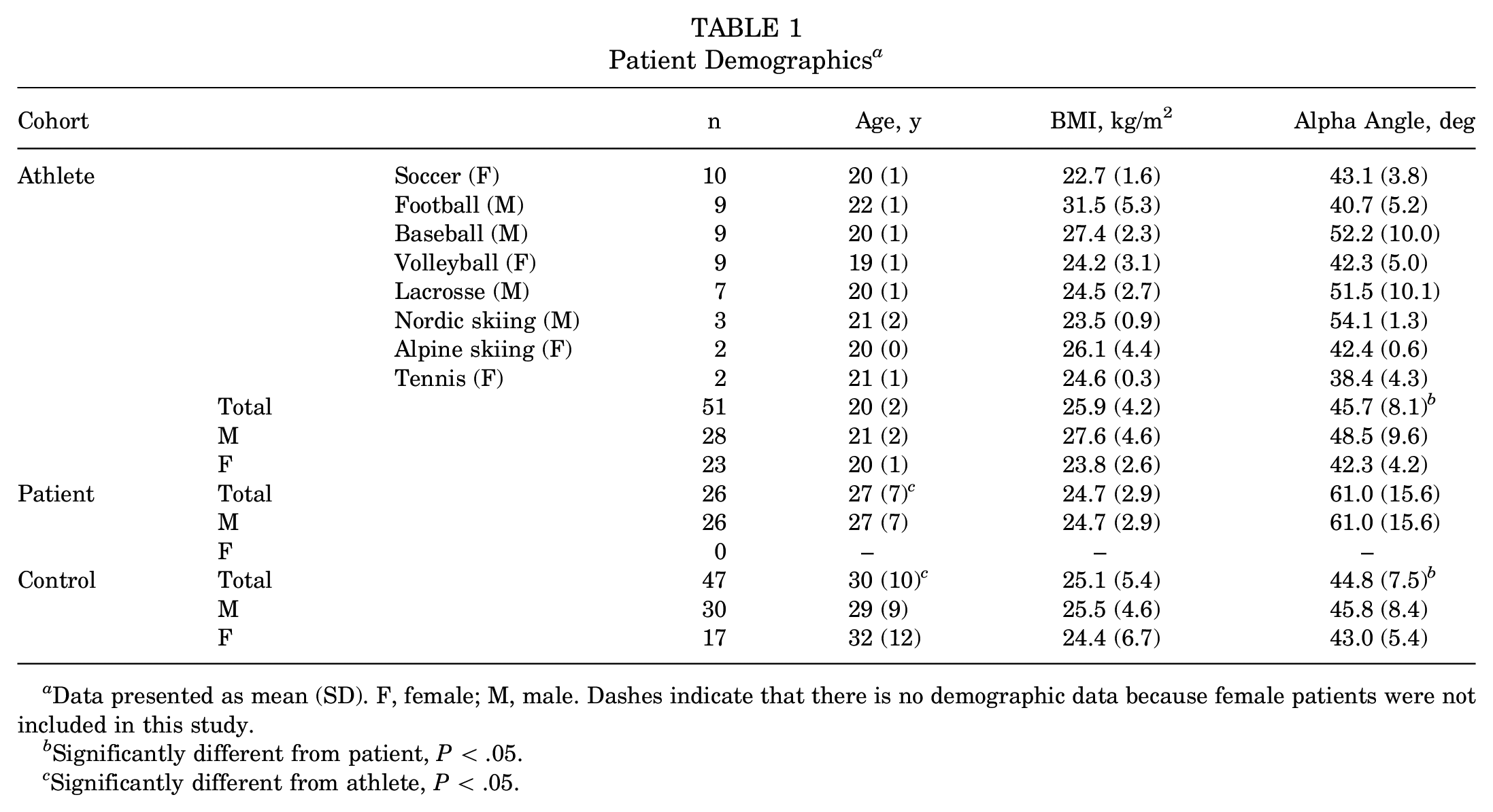
Data presented as mean (SD). F, female; M, male. Dashes indicate that there is no demographic data because female patients were not included in this study.

Significantly different from patient, P < .05.

Significantly different from athlete, P < .05.

Participant Imaging

An MRI scan of the proximal femurs was obtained for each athlete. All scanning was performed on a Siemens 3T Magnetom Prisma Fit using a 3D double echo steady state (DESS) sequence (512 × 512 × 288 matrix, 0.7-mm slice thickness, 0.7-mm³ voxel resolution, 16.3-ms repetition time, 4.7-ms echo time, and 25° flip angle). For all participants, 3D models of the proximal femur of the dominant limb were created via segmentation using Amira 6.0.1 (Thermo Fisher Scientific). The proximal femurs of controls and patients were imaged with CT and reconstructed through segmentation.^19,27,32 The previous studies used to collect the controls and patients utilized CT. To eliminate radiation exposure for volumetric imaging, we used a high-resolution MRI sequence instead. The DESS MRI sequence has been validated, with segmentation reconstructions showing accuracy similar to that of a CT.¹

Statistical Shape Modeling

Proximal femoral meshes were input to ShapeWorks 6.3.2 to generate a particle-based correspondence model (shapeworks.sci.utah.edu).^14,23 Before optimization, meshes were smoothed and decimated, reflected if right-sided, and aligned via the iterative closest point algorithm.¹⁰ Cutting planes were defined to constrain particle placement to consistent regions of the proximal femur. To do so, the best-fit cylinder to the femoral shaft was determined for each mesh. The orientation of the long axis of the cylinder defined the normal vector of the plane. Next, the first principal curvature was computed over the entirety of each mesh using FEBio Studio 1.6.1 (febio.org).³⁶ The proximodistal position of the plane was standardized using the division between the lesser trochanter and femoral shaft as visualized by the curvature map. Correspondence particles (n = 1024) were then placed at consistent anatomic sites across meshes using a fully automated hierarchical splitting strategy and entropy-based optimization.¹⁵ Generalized Procrustes analysis was used during optimization to remove the effect of pose and scale on particle position.²⁴ The suitability of the chosen sample size of 124 participants for the developed model of the proximal femur herein was tested and confirmed to be sufficient through analyses of compactness, generalization, and specificity. For SSM, these metrics can replace the approach to estimate study sample size through traditional a priori power analyses.⁴⁵ Compactness ensures the model represents the data distribution in the least number of parameters, generalization measures the ability of the model to generalize to more than just the shapes that it was optimized on, and specificity ensures that the model still represents the population.

Statistical Analysis

Demographic and radiographic variables were compared between groups via separate 1-way analyses of variance (ANOVAs) with a type 1 error rate set at .05, followed by the Tukey-Kramer method for multiple comparisons.

Principal component analysis (PCA) was used to consolidate the dimensionality of the model to a set of linearly uncorrelated modes of variation. Simply, PCA determines where variation occurs within a large, complex set of data by determining where strong patterns exist between data points. Modes of variation or modes are determined by PCA and describe the dominant shape variations among a data set. In this instance, PCA describes the variation amongst the particle sets between groups. The first mode of variation describes the most variation within the population with each subsequent mode representing less than the previous mode. Modes that represent a small percentage of the variation among the population can still encompass significant variation. PCA was performed on the correspondence particles determined by the shape model for distinct groups and subgroups of femoral surfaces, which included the following:

Group I - All participants (male and female controls, male and female athletes, and male patients)

Group II - Athletes and controls

Subgroup I - Male athletes and female athletes

Subgroup II - Female athletes and controls

Subgroup III - Male athletes and controls

Group III - Male participants only (controls, athletes, and patients)

In contrast to groups 1 and 3, group 2 (athletes and controls) was distilled down further than the cohort level to enable sex-based comparisons between athletes and controls. PCA determined modes of variation for each group and subgroup.

Modes containing significant variation were identified via parallel analysis.³⁰ Only those modes containing significant variation identified using parallel analysis were used for further statistical testing. For groups 1 and 3, 1-way ANOVA compared PCA component scores between cohorts for those modes found to be significant by parallel analysis. When ANOVA determined significant differences within a group, the Tukey-Kramer method was applied for multiple comparisons to determine which pairs exhibited significant differences. For group 2, PCA component scores were compared between cohorts for a given mode using 2-tailed unpaired t tests. Given that multiple t tests were performed for each mode, a Holm-Sidak correction was applied. Type 1 error rate was set at .05 for all statistical testing. Heat maps representing ±2 SDs from the group mean were generated for each mode describing significant variation. Heat maps were generated by measuring the Euclidean distance between the mean and ±2 SD using CloudCompare Version 2.12 (www.cloudcompare.org). Next, the distance between surfaces was measured to analyze how cohort means compared with one another. For each group and subgroup, the mean femoral shape of each cohort was determined by averaging the coordinates of each correspondence particle across individual meshes. The Euclidean distance between mean femoral meshes was measured in CloudCompare.

For the group with only male participants (group 3), linear discriminant analysis was performed to distill the high-dimensional particle data to a single numeric “shape score.” Linear discriminant analysis uses combinations of features to separate a cohort into groups based on unique features, which enables analysis and comparison of individual femoral morphologies. In our analysis, a shape score represented a generalized shape for each male participant in comparison with the mean male patient and mean male control femur. Specifically, the 1024 correspondence particles representing each participant’s femoral surface were mapped to a vector and normalized to represent the variation between the mean patient and mean control particle configurations. The linear discrimination vector was defined as the difference between the male patient and male control mean vectors. Individual participant shapes were then mapped along this vector (normalized to −1 and +1 for male patients and male controls, respectively) by taking the dot product between the participant-specific vector and linear discrimination vector. This approach has been previously applied in SSM studies to quantify overall 3D shape similarity/dissimilarity relative to cohort means on a participant-by-participant basis.^6,7 Shape scores were compared between groups via a 1-way ANOVA with type 1 error rate set at .05, followed by the Tukey-Kramer method for multiple comparisons. Linear discriminant analysis was only performed on the male cohort because female cam FAIS patients were not included in this study. All statistical analyses were performed in MATLAB 2023b (MathWorks).

Results

Age and alpha angle exhibited significant differences between cohorts (P < .0001 and P < .0001, respectively) (Table 1). Mean ± SD age was 20 ± 2 years, 27 ± 7 years, and 30 ± 10 years for 51 athletes, 26 patients, and 47 controls, respectively. The age of athletes was significantly less than that of patients (adjusted P = .0003) and controls (adjusted P < .0001). Mean ± SD alpha angles were 45.7°± 8.1°, 61.0°± 15.6°, and 44.8°± 7.5° for athletes, patients, and controls, respectively. The alpha angle of patients was significantly greater than athletes (adjusted P < .0001) and controls (adjusted P < .0001). Mean ± SD BMI was 25.9 ± 4.2 kg/m², 24.7 ± 2.9 kg/m², and 25.1 ± 5.4 kg/m² for athletes, patients, and controls, respectively. BMI was not significantly different between athletes and controls, athletes and patients, or patients and controls.

All Participants (Group 1)

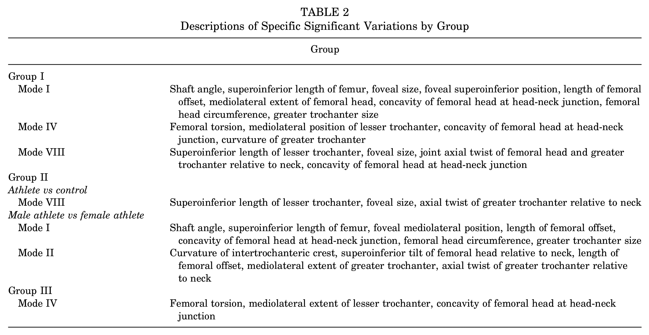
Considering all participants collectively, parallel analysis identified the first 8 PCA modes as having statistically significant shape variations (modes I-VIII accounted for 80.5% of the cumulative variance, with the modes separately describing 33.4%, 16.9%, 11%, 6.5%, 5.2%, 3.2%, 2.6%, and 1.8% of the variance, respectively). However, only modes I, IV, and VIII exhibited significant between-group differences in PCA scores (P = .004, P = .0006, and P = .0007, respectively). Specifically, between athletes and controls, PCA scores for only mode VIII were significantly different (adjusted P = .01); between athletes and patients, modes I and IV were significantly different (adjusted P = .002 and adjusted P = .003, respectively), and between patients and controls, modes IV and VIII were significantly different (adjusted P = .0003 and adjusted P = .0007, respectively). These modes highlighted variation in femoral offset, the concavity of the femoral head at the head-neck junction, and the length of the lesser trochanter, among other minor regions (Figure 1). A detailed description of the specific locations where variation occurred can be found in Table 2. Cohort differences, as represented by a color fringe plot (Figure 2), showed shape differences ranging from 0.6 mm to 2.5 mm.

Figure 1.

Posteromedial (left column) and superior (right column) views of distance maps representing the mean and ±2 SD of the modes of variation that exhibited significant pairwise differences when considering all participants (modes I, IV, and VIII). White represents the mean shape, and the positive (purple) and negative (orange) values represent areas where the SD extended beyond the mean and where the SD was not as pronounced as the mean, respectively. Significant modes highlighted variation at the femoral head-neck junction.

Table 2

Descriptions of Specific Significant Variations by Group

Group
Group I
Mode I	Shaft angle, superoinferior length of femur, foveal size, foveal superoinferior position, length of femoral offset, mediolateral extent of femoral head, concavity of femoral head at head-neck junction, femoral head circumference, greater trochanter size
Mode IV	Femoral torsion, mediolateral position of lesser trochanter, concavity of femoral head at head-neck junction, curvature of greater trochanter
Mode VIII	Superoinferior length of lesser trochanter, foveal size, joint axial twist of femoral head and greater trochanter relative to neck, concavity of femoral head at head-neck junction
Group II
Athlete vs control
Mode VIII	Superoinferior length of lesser trochanter, foveal size, axial twist of greater trochanter relative to neck
Male athlete vs female athlete
Mode I	Shaft angle, superoinferior length of femur, foveal mediolateral position, length of femoral offset, concavity of femoral head at head-neck junction, femoral head circumference, greater trochanter size
Mode II	Curvature of intertrochanteric crest, superoinferior tilt of femoral head relative to neck, length of femoral offset, mediolateral extent of greater trochanter, axial twist of greater trochanter relative to neck
Group III
Mode IV	Femoral torsion, mediolateral extent of lesser trochanter, concavity of femoral head at head-neck junction

Figure 2.

Distance maps illustrating shape differences between the mean shapes of specified cohort pairs for all participants (left column), athletes and controls (middle column), and males (right column). The first cohort in each pair is mapped on the second, showing areas where the first cohort differs from the second. Purple and orange represent areas where the first cohort extended beyond the second cohort and areas where the first cohort was not as pronounced as the second cohort, respectively. The greatest differences between pairs commonly occurred at the head-neck junction. F, female; M, male.

Athletes and Controls (Group 2)

Athlete Versus Control (Group 2)

Considering athletes and controls only, parallel analysis identified the first 8 PCA modes as having statistically significant shape variations (modes I-VIII accounted for 80.7% of the cumulative variance, with the modes separately describing 32%, 18.1%, 10.9%, 6.2%, 5.3%, 3.3%, 2.8%, and 2% of the variation, respectively). PCA component scores for mode VIII exhibited significant differences between athletes and controls (adjusted P = .04) (Figure 3). Significant modes highlighted variation in the length of the lesser trochanter. A detailed description of the specific locations where variation occurred can be found in Table 2. Cohort differences, as represented by a color fringe plot (Figure 2), showed notable shape differences ranging from 1.2 mm to 1.5 mm.

Figure 3.

Posteromedial (left column) and superior (right column) views of distance maps representing the mean and ±2 SD of the mode that exhibited significant pairwise differences when considering all athletes and controls (mode VIII). White represents the mean shape, and the positive (purple) and negative (orange) values represent areas where the SD extended beyond the mean and where the SD was not as pronounced as the mean, respectively. Mode VIII primarily highlights variation in the lesser trochanter.

Male Athlete Versus Female Athlete (Subgroup 1)

Considering male athletes and female athletes only, parallel analysis identified the first 6 PCA modes as having statistically significant shape variations (modes I-VI accounted for 78.5% of the cumulative variance, with the modes separately describing 31.7%, 17.9%, 13.8%, 6.4%, 5.2%, and 3.5%, respectively). PCA component scores for modes I and II exhibited significant differences between male and female athletes (adjusted P = .006 and adjusted P = .009, respectively) (Figure 4). Significant modes highlighted variation in femoral offset and concavity of the femoral head at the head-neck junction. A detailed description of the specific locations where variation occurred can be found in Table 2. Cohort differences, as represented by a color fringe plot (Figure 2), showed shape differences ranging from 1.0 mm to 2.4 mm throughout the entire proximal femur.

Figure 4.

Posteromedial (left column) and superior (right column) views of distance maps of the mean and ±2 SD of the modes that exhibited significant differences between male and female athletes (modes I and II). White represents the mean shape, and the positive (purple) and negative (orange) values represent areas where the SD extended beyond the mean and where the SD was not as pronounced as the mean, respectively. The significant modes primarily highlight variation in the greater trochanter, head-neck junction, and the length of the proximal femur.

Female Athlete Versus Female Control (Subgroup 2)

Considering female athletes and female controls only, parallel analysis identified the first 5 PCA modes as having statistically significant shape variations (modes I-V accounted for 73.8% of the cumulative variance, with the modes separately describing 30.7%, 15.6%, 13.3%, 8.3%, and 5.9%, respectively). PCA component scores were not significantly different between female athletes and controls. Cohort differences, as represented by a color fringe plot (Figure 2), showed shape differences ranging from 0.7 mm to 2.2 mm.

Male Athlete Versus Male Control (Subgroup 3)

Considering male athletes and male controls only, parallel analysis identified the first 7 PCA modes as having statistically significant shape variations (modes I-VII accounted for 79.6% of the cumulative variance, with the modes separately describing 31.9%, 18.1%, 11.2%, 6.2%, 5.3%, 3.8%, and 3.3%, respectively). PCA component scores were not significantly different between male athletes and male controls. Cohort differences, as represented by a color fringe plot (Figure 2), showed no notable differences between male athletes and male controls.

Male Participants Only (Group 3)

Considering male participants only, parallel analysis identified the first 7 PCA modes as having statistically significant shape variations (modes I-VII accounted for 78.8% of the cumulative variance, with the modes separately describing 32.3%, 17.1%, 11.2%, 6.6%, 5.3%, 3.6%, and 2.7% of shape variation, respectively). PCA component scores for mode IV exhibited significant group differences (P = .002). Post hoc analysis determined that differences were between athletes and patients (adjusted P = .02) and patients and controls (adjusted P = .003) (Figure 5). Mode IV highlighted variation in the concavity of the femoral head at the head-neck junction and femoral torsion. A detailed description of the specific locations where variation occurred can be found in Table 2. Cohort differences, as represented by a color fringe plot (Figure 2), showed shape differences ranging from 0.5 mm to 2.3 mm.

Figure 5.

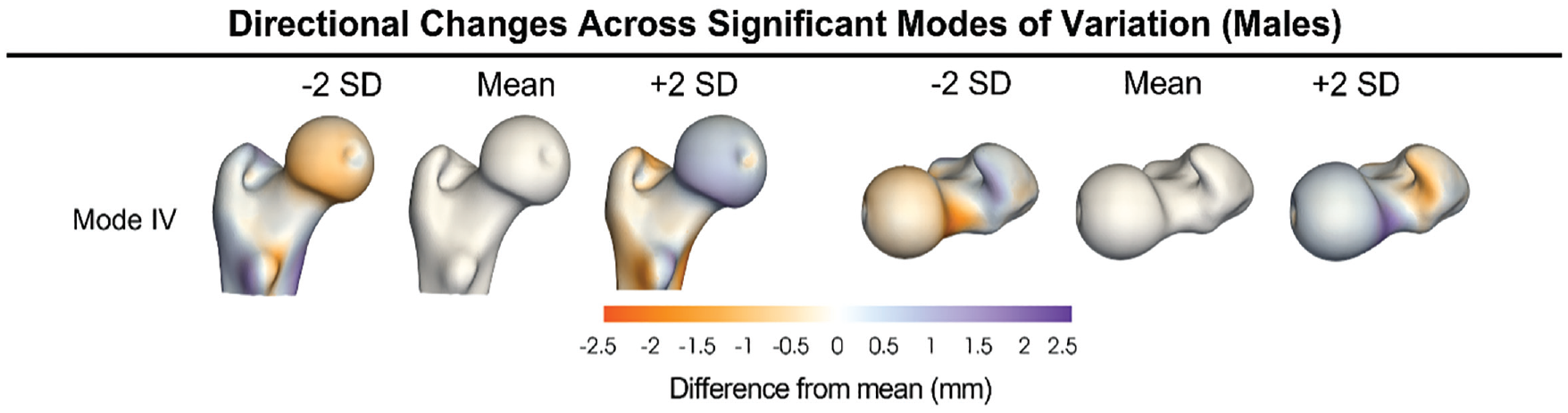
Posteromedial (left column) and superior (right column) views of distance maps representing the mean and ±2 SD of the modes of variation that exhibited significant pairwise differences when considering male participants (mode IV). White represents the mean shape, and the positive (purple) and negative (orange) values represent areas where the SD extended beyond the mean and where the SD was not as pronounced as the mean, respectively. Variation in male participants is primarily observed in the rotation of the femur and at the head-neck junction.

Significant group differences in overall 3D shape were identified by linear discriminant analysis (P < .0001). The mean ± SD of shape scores among athletes, patients, and controls were 0.4 ± 1.6, –1.0 ± 1.7, and 1.0 ± 1.4, respectively. Shape scores were significantly different between athletes and patients (adjusted P = .003) and patients and controls (adjusted P < .0001) but not athletes and controls (adjusted P = .40) (Figure 6). Six out of 9 baseball players exhibited negative shape scores indicating more cam-like morphology, whereas 8 of 9 football players and 5 of 7 lacrosse players exhibited positive scores indicating more control-like morphology (Figure 7). Most athletes (64%) fell between a shape score of 0 and 5 (mean ± SD, 0.4 ± 1.6), indicative of a control-leaning shape score. Select athletes (32%) had shape scores indicative of patient-leaning anatomy. Alpha angle, but not BMI, exhibited a fair to moderate correlation with shape score (rho = −0.55) (Figure 8).

Figure 6.

Histogram of male control (black), male athlete (white), and male patient (gray) shape scores as determined by linear discriminant analysis. The bars on the right (asterisks) represent a significant difference between cohorts.

Figure 7.

Surface reconstructions representing the mean shape of the male patient (blue), male control (gray), and male athlete (red) proximal femur, as well as sports icons representing each individual athlete’s shape score as determined by linear discriminant analysis. Positive shape scores indicate femurs resembling controls, and negative shape scores indicate femurs resembling patients. Horizontal dotted lines represent the SD for each group. Vertical lines (asterisks) indicate a significant difference between athletes and patients and controls and patients. Significant differences in shape were found between patients versus controls and patients versus athletes among male participants.

Figure 8.

(A) Scatterplot illustrating the moderate negative correlation (rho = −0.55; P < .001) between alpha angle and shape score in male participants. (B) Scatterplot illustrating no significant relationship (rho = 0.04; P = .71) between body mass index (BMI) and shape score.

Discussion

Recent studies have used 2D SSM, radiographic measurements, and linear regression to assess the correlation between femoral shape and the presence of cartilage defects in athletes.^29,47 However, this is the first study to our knowledge to use 3D SSM techniques to quantify the proximal femoral shape and shape variation in collegiate athletes, controls screened for cam morphology, and cam-type FAIS patients together. The results of our 3D SSM demonstrated significant modes of variation between studied cohorts that described femoral offset, concavity, and mediolateral extent of the femoral head and trochanter size and location. These regions of the proximal femur correspond to clinical observations of cam morphology, but with a higher level of fidelity and detail than that offered by measurements of plain film radiographs alone. As such, we posit that SSM could be used as a valuable clinical screening tool to evaluate deformities in athletes who are at risk of developing cam FAIS. A key finding from our analysis is that athletes had proximal femoral morphology that more closely resembled that of controls screened for cam morphology. This key finding contradicts previous studies investigating the prevalence of cam morphology in asymptomatic athletes that were based on 2D measurements of plain film radiographs.^31,33,40,46

Previous studies have examined the radiographic prevalence of cam morphology in asymptomatic baseball and football players.^31,37,46 We found that 67% (6/9) of baseball players had patient-leaning shape scores, which is consistent with the results of a previous study that showed approximately 70% of baseball players had ≥1 radiographic sign of cam morphology.⁴⁶ However, in our study, the vast majority of football players (89%; 8/9) had a control-leaning shape score, whereas Kapron et al³¹ reported that approximately 75% of football players in their study had ≥1 radiographic sign of cam morphology. The disparities between our study and previous studies examining football players may be due to a few factors. First, measurements of plain film radiographs may not accurately describe the cam deformity.⁷ As such, deformities observed on plain film radiographs may not be as severe as once predicted. Another reason for the discrepancy in results is that we used a higher threshold to define cam morphology in controls (>60°), whereas the aforementioned studies used >50° or >55°.^31,37,46 Still, none of the football players in our study had an alpha angle >55°. It is possible that we had too few football players, which created a selection bias that effectively skewed the SSM results toward more control-leaning anatomy. Additionally, a selection bias could have also been created due to our screening protocols for BMI, which excluded participants with a BMI >40 kg/m². However, it is also possible that previous studies overestimated cam deformities due to lack of reliability in radiographic measurements. SSM is more specific and represents a more accurate measurement of deformity.

Males and females exhibit distinct hip shapes due to a range of biological needs.²⁰ This may explain why the anatomical appearance of cam lesions differs between male and female participants and may clarify why athletes develop cam FAIS at different rates between the sexes.^12,34,49 In our study, PCA determined modes I and II (male and female athlete subgroup) to exhibit significant differences in shape between male and female athletes. These modes highlighted differences in the shape of the femoral head, concavity of the head-neck junction, and amount of femoral offset. SSM enhanced our ability to visualize differences and objectively analyze areas of variation that are typically associated with cam morphology.

Limitations

There are limitations in our study that warrant consideration. First, only the proximal femur was analyzed. While the proximal femur is where cam morphology occurs, the shape of the acetabulum and distal femur may also play important roles in the development of symptomatic hip impingement. Additionally, studies suggest that femoral version contributes to the development of impingement.^5,11,22,43 By confining our analysis solely to the proximal femur, we acknowledge that we are overlooking aspects of the anatomy that may contribute to the development of FAIS. Future research could evaluate the entire pelvis, the full length of the femur, and the hip joint using SSM. Second, surfaces were generated from 2 different imaging modalities, CT (controls and patients) and MRI (athletes), which could theoretically lead to differences in shape due to segmentation/reconstruction quality. However, a previous study by Abraham et al¹ determined that the accuracy of reconstructions from DESS MRI were comparable with those based on CT. Third, we used an older data set of patients with FAIS that had only 4 female patients. Given the small sample, we chose to exclude female patients from this study. It was previously thought that cam FAIS/morphology was primarily identified in males; however, recent research has shown that cam morphology is prevalent in females as well.^35,48 Additionally, each sport evaluated herein included athletes from a single sex. Comparisons of female athletes with female patients along with comparisons of both sexes between a single sport should be examined as part of future research. Finally, only Division I collegiate athletes were included in the study. Exclusive evaluation of collegiate athletes may have introduced a bias since they may not be representative of all athletes. The elite nature of these athletes may represent a worst-case scenario of higher level and sustained athletic participation, which would, in theory, maximize femoral deformities related to athletic participation. It is possible that many high-performing athletes with cam morphology become symptomatic, whereas more recreational athletes with cam morphology can continue their sport. Future work would benefit from the inclusion of skeletally immature as well as senior athletes, as analysis of these individuals would provide additional insight into the development and progression of FAIS across the athlete’s lifespan.

Implementation of a 3D diagnostic tool for identifying cam deformities in clinic would require a more automatic pipeline for reconstruction and statistical shape analysis than that utilized in our study. Recent advancements in automatic segmentation and new methods for cam deformity identification show promise in this regard. Bugeja et al¹³ developed an algorithm to automatically segment cam deformities from MRIs and identify the size of a cam deformity. Guidetti et al²⁶ developed a method to automatically identify the region of a cam deformity by noninvasively fitting femurs with cam deformities to a general femoral shape. Currently, we are working on a deep-learning approach to SSM for which correspondence points are automatically placed on anatomy directly from image data, obviating the need for segmentation and optimization to place correspondence particles on the anatomy. This approach would enable efficient SSM evaluations of femoral anatomy on a per-patient basis.

Conclusion

This study used SSM to characterize shape and shape variation in the proximal femur in asymptomatic Division I collegiate athletes. We determined that the athletes in our study had femurs that resemble control femurs that had been screened for cam morphology, which refutes previously published research. Our results provide evidence that SSM allows us to analyze regions of the femur that 2D radiographic measurements may not capture. Utilizing SSM, we can objectively analyze the 3D femoral morphology of athletes to identify and better understand morphology that may predispose individuals to FAIS. Future studies should include the pelvis, entire femur, and a larger sampling of athletes as part of the SSM to better understand the role of deformities in the development of FAIS in athletes.

Footnotes

Final revision submitted July 26, 2024; accepted July 31, 2024.

One or more of the authors has declared the following potential conflict of interest or source of funding: This study received funding from the PAC-12 Student Athlete Health and Well-Being Initiative and the National Institutes of Health under grant No. NIBIB-U24EB029011, NIBIB-R01EB016701, NIAMS-R01AR076120, NHLBI-R01HL135568, NIGMS-P41GM103545, and R24 GM136986. K.B.F. has received education payments from Intuitive Surgical. S.K.A. has received consulting fees from Stryker. T.G.M. has received nonconsulting fees from Arthrex, consulting fees from Arthrex, and education payments from Active Medical. AOSSM checks author disclosures against the Open Payments Database (OPD). AOSSM has not conducted an independent investigation on the OPD and disclaims any liability or responsibility relating thereto.

Ethical approval for this study was obtained from the University of Utah (IRB No. 00109768).

References

Abraham

Bangerter

McGavin

, et al. Accuracy of 3D dual echo steady state (DESS) MR arthrography to quantify acetabular cartilage thickness. J Magn Reson Imaging. 2015;42(5):1329-1338.

Agricola

Bessems

JHJM

Ginai

, et al. The development of cam-type deformity in adolescent and young male soccer players. Am J Sports Med. 2012;40(5):1099-1106.

Agricola

Heijboer

Roze

, et al. Pincer deformity does not lead to osteoarthritis of the hip whereas acetabular dysplasia does: acetabular coverage and development of osteoarthritis in a nationwide prospective cohort study (CHECK). Osteoarthritis Cartilage. 2013;21(10):1514-1521.

Anderson

Kapron

, et al. The 2015 Frank Stinchfield Award: radiographic abnormalities common in senior athletes with well-functioning hips but not associated with osteoarthritis. Clin Orthop Relat Res. 2016;474(2):342-352.

Arshad

Maughan

Sunil Kumar

Pettit

Arora

Khanduja

Over one third of patients with symptomatic femoroacetabular impingement display femoral or acetabular version abnormalities. Knee Surg Sports Traumatol Arthrosc. 2021;29(9):2825-2836.

Atkins

Elhabian

Agrawal

, et al. Quantitative comparison of cortical bone thickness using correspondence-based shape modeling in patients with cam femoroacetabular impingement. J Orthop Res. 2017;35(8):1743-1753.

Atkins

Shin

Agrawal

, et al. Which two-dimensional radiographic measurements of cam femoroacetabular impingement best describe the three-dimensional shape of the proximal femur? Clin Orthop Relat Res. 2019;477(1):242-253.

Barton

Salineros

Rakhra

Beaulé

PE.

Validity of the alpha angle measurement on plain radiographs in the evaluation of cam-type femoroacetabular impingement. Clin Orthop Relat Res. 2011;469(2):464-469.

Beck

Kalhor

Leunig

Ganz

Hip morphology influences the pattern of damage to the acetabular cartilage. J Bone Joint Surg Br. 2005;87(7):1012-1018.

10.

Besl

McKay

ND.

A method for registration of 3-D shapes. IEEE Trans Pattern Anal Mach Intell. 1992;14(2):239-256.

11.

Boschung

Antioco

Novais

, et al. Large hip impingement area and subspine hip impingement in patients with absolute femoral retroversion or decreased combined version. Orthop J Sports Med. 2023;11(2):23259671221148502.

12.

Bugeja

Xia

Chandra

, et al. Analysis of cam location characteristics in FAI syndrome patients from 3D MR images demonstrates sex-specific differences. J Orthop Res. 2024;42(2):385-394.

13.

Bugeja

Xia

Chandra

, et al. Automated volumetric and statistical shape assessment of cam-type morphology of the femoral head-neck region from clinical 3D magnetic resonance images. Quant Imaging Med Surg. 2022;12(10):4924-4941.

14.

Cates

Elhabian

Whitaker

. Chapter 10—ShapeWorks: particle-based shape correspondence and visualization software. In: Zheng

Székely

, eds. Statistical Shape and Deformation Analysis. Academic Press; 2017:257-298.

15.

Cates

Fletcher

Styner

Shenton

Whitaker

Shape modeling and analysis with entropy-based particle systems. Inf Process Med Imaging. 2007;20:333-345.

16.

Clohisy

Carlisle

Trousdale

, et al. Radiographic evaluation of the hip has limited reliability. Clin Orthop Relat Res. 2009;467(3):666-675.

17.

Dudda

Albers

Mamisch

Werlen

Beck

Do normal radiographs exclude asphericity of the femoral head-neck junction?

Clin Orthop Relat Res. 2009;467(3):651-659.

18.

Ecker

Tannast

Puls

Siebenrock

Murphy

SB.

Pathomorphologic alterations predict presence or absence of hip osteoarthrosis. Clin Orthop Relat Res. 2007;465:46-52.

19.

Fiorentino

Kutschke

Atkins

Foreman

Kapron

Anderson

AE.

Accuracy of functional and predictive methods to calculate the hip joint center in young non-pathologic asymptomatic adults with dual fluoroscopy as a reference standard. Ann Biomed Eng. 2016;44(7):2168-2180.

20.

Fischer

Mitteroecker

Allometry and sexual dimorphism in the human pelvis. Anat Rec (Hoboken). 2017;300(4):698-705.

21.

Ganz

Parvizi

Beck

Leunig

Nötzli

Siebenrock

KA.

Femoroacetabular impingement: a cause for osteoarthritis of the hip. Clin Orthop Relat Res. 2003;417:112-120.

22.

Goldsmith

Cheng

Mintz

Moley

Correlation of femoral version measurements between computed tomography and magnetic resonance imaging studies in patients presenting with a femoroacetabular impingement-related complaint. J Hip Preserv Surg. 2022;9(4):219-224.

23.

Goparaju

Iyer

Bône

, et al. Benchmarking off-the-shelf statistical shape modeling tools in clinical applications. Med Image Anal. 2022;76:102271.

24.

Gower

JC.

Generalized procrustes analysis. Psychometrika. 1975;40(1):33-51.

25.

Griffin

Dickenson

O’Donnell

, et al. The Warwick Agreement on femoroacetabular impingement syndrome (FAI syndrome): an international consensus statement. Br J Sports Med. 2016;50(19):1169-1176.

26.

Guidetti

Malloy

Alter

Newhouse

Nho

Espinoza Orías

AA.

Noninvasive shape-fitting method quantifies cam morphology in femoroacetabular impingement syndrome: implications for diagnosis and surgical planning. J Orthop Res. 2023;41(6):1256-1265.

27.

Harris

Datar

Whitaker

Jurrus

Peters

Anderson

AE.

Statistical shape modeling of cam femoroacetabular impingement. J Orthop Res. 2013;31(10):1620-1626.

28.

Harris

Kapron

Peters

Anderson

AE.

Correlations between the alpha angle and femoral head asphericity: implications and recommendations for the diagnosis of cam femoroacetabular impingement. Eur J Radiol. 2014;83(5):788-796.

29.

Heerey

Kemp

Agricola

, et al. Cam morphology is associated with MRI-defined cartilage defects and labral tears: a case-control study of 237 young adult football players with and without hip and groin pain. BMJ Open Sport Exerc Med. 2021;7(4):e001199.

30.

Horn

JL.

A rationale and test for the number of factors in factor analysis. Psychometrika. 1965;30(2):179-185.

31.

Kapron

Anderson

Aoki

, et al. Radiographic prevalence of femoroacetabular impingement in collegiate football players: AAOS exhibit selection. J Bone Joint Surg Am. 2011;93(19):e111.

32.

Kapron

Aoki

Peters

Anderson

AE.

In-vivo hip arthrokinematics during supine clinical exams: application to the study of femoroacetabular impingement. J Biomech. 2015;48(11):2879-2886.

33.

Kapron

Peters

Aoki

, et al. The prevalence of radiographic findings of structural hip deformities in female collegiate athletes. Am J Sports Med. 2015;43(6):1324-1330.

34.

Kopec

Hong

Wong

, et al; IMPAKT-HIP Study Team. Prevalence of femoroacetabular impingement syndrome among young and middle-aged white adults. J Rheumatol. 2020;47(9):1440-1445.

35.

Levy

Hellman

Harris

Haughom

Frank

Nho

SJ.

Prevalence of cam morphology in females with femoroacetabular impingement. Front Surg. 2015;2:61.

36.

Maas

Ellis

Ateshian

Weiss

JA.

FEBio: finite elements for biomechanics. J Biomech Eng. 2012;134(1):11005.

37.

Nepple

Brophy

Matava

Wright

Clohisy

JC.

Radiographic findings of femoroacetabular impingement in National Football League Combine athletes undergoing radiographs for previous hip or groin pain. Arthroscopy. 2012;28(10):1396-1403.

38.

Nepple

Martel

Kim

Zaltz

Clohisy

JC.

Do plain radiographs correlate with CT for imaging of cam-type femoroacetabular impingement?

Clin Orthop Relat Res. 2012;470(12):3313-3320.

39.

Philippon

Schenker

Briggs

Kuppersmith

Femoroacetabular impingement in 45 professional athletes: associated pathologies and return to sport following arthroscopic decompression. Knee Surg Sports Traumatol Arthrosc. 2007;15(7):908-914.

40.

Philippon

Briggs

Stull

LaPrade

RF.

Prevalence of increased alpha angles as a measure of cam-type femoroacetabular impingement in youth ice hockey players. Am J Sports Med. 2013;41(6):1357-1362.

41.

Riley

McWalter

Stevens

Safran

Lattanzi

Gold

GE.

MRI of the hip for the evaluation of femoroacetabular impingement; past, present, and future. J Magn Reson Imaging. 2015;41(3):558-572.

42.

Safran

Foard

Robell

Pullen

WM.

Incidence of symptomatic femoroacetabular impingement: a 4-year study at a National Collegiate Athletic Association Division I institution. Orthop J Sports Med. 2022;10(4):23259671221084979.

43.

Schaver

Oshodi

Glass

Duchman

Willey

Westermann

RW.

Cam morphology is associated with increased femoral version: findings from a collection of 1,321 cadaveric femurs. Arthroscopy. 2022;38(3):831-836.

44.

Scholes

Kemp

Mentiplay

, et al. Are cam morphology size and location associated with self-reported burden in football players with FAI syndrome? Scand J Med Sci Sports. 2022;32(4):737-753.

45.

Styner

Rajamani

Nolte

, et al. Evaluation of 3D correspondence methods for model building. Inf Process Med Imaging. 2003;18:63-75.

46.

Uquillas

Sun

Van Sice

ElAttrache

Banffy

MB.

Prevalence of femoroacetabular impingement in elite baseball players. J Hip Preserv Surg. 2022;9(3):145-150.

47.

van Buuren

MMA

Heerey

Smith

, et al. The association between statistical shape modeling-defined hip morphology and features of early hip osteoarthritis in young adult football players: data from the femoroacetabular impingement and hip osteoarthritis cohort (FORCe) study. Osteoarthr Cartil Open. 2022;4(3):100275.

48.

Yanke

Khair

Stanley

, et al. Sex differences in patients with CAM deformities with femoroacetabular impingement: 3-dimensional computed tomographic quantification. Arthroscopy. 2015;31(12):2301-2306.

49.

Zhou

Melugin

Hale

, et al. Sex differences in the prevalence of radiographic findings of structural hip deformities in patients with symptomatic femoroacetabular impingement. J Hip Preserv Surg. 2021;8(3):233-239.

Cam Morphology and Sex-Based Differences in the Proximal Femur Anatomy of Collegiate Athletes Without Hip Pain: A 3-Dimensional Statistical Shape Modeling Analysis

Abstract

Background:

Purpose:

Study Design:

Methods:

Results:

Conclusion:

Keywords

Methods

Participants

Participant Imaging

Statistical Shape Modeling

Statistical Analysis

Results

All Participants (Group 1)

Athletes and Controls (Group 2)

Athlete Versus Control (Group 2)

Male Athlete Versus Female Athlete (Subgroup 1)

Female Athlete Versus Female Control (Subgroup 2)

Male Athlete Versus Male Control (Subgroup 3)

Male Participants Only (Group 3)

Discussion

Limitations

Conclusion

Footnotes

References