Sage Journals: Discover world-class research

Abstract

Background:

The opportunity to quantitatively predict next-season injury risk in the National Hockey League (NHL) has become a reality with the advent of advanced computational processors and machine learning (ML) architecture. Unlike static regression analyses that provide a momentary prediction, ML algorithms are dynamic in that they are readily capable of imbibing historical data to build a framework that improves with additive data.

Purpose:

To (1) characterize the epidemiology of publicly reported NHL injuries from 2007 to 2017, (2) determine the validity of a machine learning model in predicting next-season injury risk for both goalies and position players, and (3) compare the performance of modern ML algorithms versus logistic regression (LR) analyses.

Study Design:

Descriptive epidemiology study.

Methods:

Professional NHL player data were compiled for the years 2007 to 2017 from 2 publicly reported databases in the absence of an official NHL-approved database. Attributes acquired from each NHL player from each professional year included age, 85 performance metrics, and injury history. A total of 5 ML algorithms were created for both position player and goalie data: random forest, K Nearest Neighbors, Naïve Bayes, XGBoost, and Top 3 Ensemble. LR was also performed for both position player and goalie data. Area under the receiver operating characteristic curve (AUC) primarily determined validation.

Results:

Player data were generated from 2109 position players and 213 goalies. For models predicting next-season injury risk for position players, XGBoost performed the best with an AUC of 0.948, compared with an AUC of 0.937 for LR (P < .0001). For models predicting next-season injury risk for goalies, XGBoost had the highest AUC with 0.956, compared with an AUC of 0.947 for LR (P < .0001).

Conclusion:

Advanced ML models such as XGBoost outperformed LR and demonstrated good to excellent capability of predicting whether a publicly reportable injury is likely to occur the next season.

Keywords

NHL machine learning regression injury prediction

Ice hockey is one of the fastest and most physical team sports in the world.⁶ With players reaching speeds of up to 30 miles per hour, puck speeds reaching 100 miles per hour, and an ingrained cultural encouragement of physical contact and aggressive play, the risk of injury in ice hockey played at any level of competition is very high.^9,16,26 To mitigate injury risk and increase the availability of these elite athletes, professional hockey teams invest millions of dollars per year on injury prevention.²⁰ In the National Hockey League (NHL), the premier ice hockey league in the world, injuries are estimated to cost the league $218 million in missed player time every year, with concussion alone costing $42.8 million a year.¹¹ In a league where teams are challenged to obtain any incremental competitive advantage, the ability to quantitatively predict which players are most vulnerable to injury at a given moment represents a promising possibility.¹⁴ For this purpose, machine learning may be a suitable tool.

Machine learning, a subset of artificial intelligence, is the application of computational algorithms that can recognize patterns in data without explicit human instruction or supervision.^3,5 From these data, patterns and inferences are incorporated into the creation of intelligent, predictive models. In essence, machine learning is a technique that is capable of analyzing large sets of data, learning from historical data to make predictions about the future.^3,5,22 First, real-world data sets are divided into “training sets” and “test sets.” The training sets are fed into machine learning models, which recognize subtle patterns in the data. Then, the accuracy of the algorithm is assessed with a test set, whose outcomes are already known and can be compared with the output of the algorithm. With larger training sets and an increased number of training/testing repetitions, these algorithms can self-correct and reach higher levels of predictive accuracy.⁵

Previous research has examined the application of machine learning techniques to the NHL. In 2019, Gu et al¹³ described an expert system that used a support vector machine to predict game outcomes. In 2015, Demers¹⁰ compared the performance of 2 Stanley Cup prediction systems using a relevance vector machine algorithm and a support vector machine algorithm. In these studies, machine learning concepts were applied with the goal of accurately predicting the outcomes of hockey games. However, research is lacking on the use of machine learning to predict future injuries in professional hockey players, likely because of the absence of an official centralized NHL injury reporting database. To the end of leveraging available analytics to permit data-driven injury prevention strategies and informed decisions for NHL franchises beyond supervised logistic regression analysis, the objective of this study of NHL players was to (1) characterize the epidemiological patterns of publicly reported NHL injuries from 2007 to 2017, (2) determine the validity of a machine learning model in predicting next-season injury risk for both goalies and position players, and (3) compare the performance of modern machine learning algorithms versus logistic regression analyses. We hypothesized that an algorithm, trained on previous injury history, player performance metrics, and player characteristics, would be able to predict the likelihood of a player being injured in the subsequent season of play.

Methods

Injury data for players in the NHL from the years 2007 to 2017 were compiled from the Pro Sports Transactions²¹ archives in the absence of an official NHL-approved database. Relevant data included player name, team at the time of injury, date of the injury, and descriptive characteristics of the injury. Because date of return was not reported, we could not document overall time or games missed. Although Pro Sports Transactions is not officially regulated by the NHL, the database is widely considered reliable, and several previous studies have used data from Pro Sports Transactions over its 15-year history.^4,27 Performance and player availability metrics were compiled from Hockey Reference,¹⁷ a publicly accessible website. These data were systematically extracted using a custom Python (Version 3.7.3; Python Software Foundation) script. Injuries were designated as day-to-day injuries versus more interruptive injuries. Raw data were compiled using R (Version 3.5.1; R Foundation for Statistical Computing) and Python. All player injuries were grouped by year and totaled to arrive at the total number of injuries for each year. These data were then matched with player statistics for each season, resulting in a list of player statistics and injuries for each season players were in the NHL. Table 1 further explains the technical machine learning terms and concepts.

TABLE 1

Definitions of Machine Learning Terms and Concepts

Term	Definition
Variance inflation factor (VIF)	A measure of multicollinearity in a regression analysis. A higher VIF indicates that predictors are highly correlated with each other, generally indicating a less reliable result.
Python StatsModel package	A Python module that provides resources for conducting statistical analysis in Python.
K Nearest Neighbors	A pattern recognition algorithm used for both classification and regression. This algorithm classifies a case based on the classification of a majority of its neighbors.
Naïve Bayes	An algorithm that classifies cases based on the application of Bayes’ theorem with the assumption of conditional independence.
XGBoost	A machine learning algorithm that uses a gradient boosting framework to solve prediction problems.
Top 3 Ensemble	An ensemble algorithm that incorporates multiple machine learning algorithms (top 3) to augment predictive performance.
Broyden-Fletcher-Goldfarb-Shanno optimizer	An iterative algorithm that allows for the solving of unconstrained optimization problems.
Brier score loss	A calculation of the mean squared error between predicted and expected values. A low Brier score indicates better predictions.
Area under the curve (AUC) of the receiver operating characteristic curve	An aggregate measure of a model’s classification performance. AUC ranges in value from 0 to 1.0, with an AUC 1 meaning that a model is capable of distinguishing between classes 100% of the time.
Shapley Additive Explanations (SHAP) score	A measure of feature importance in predictive modeling. A higher SHAP value indicates a factor that predicts higher injury probability, whereas a lower SHAP value indicates a factor that predicts a lower injury probability.

Data Processing and Feature Selection

Data attributes were selected from the model for each player. All predictor variables used in the model were assessed for multicollinearity using the variance inflation factor (VIF) for each variable in an ordinary-least-squares regression context using the Python StatsModel package.²⁵ In doing so, we identified 23 variables with a VIF of >10 that did not contribute to the predictive power of the model but did increase its variance²³ and thus were excluded from the model in a sequential fashion until all variables had a VIF ≤10. Final features selected for position players and goalies can be found in Appendix Tables A1 and A2.

Machine Learning Model: Development and Validation

Machine learning modeling was performed on a Macintosh computer with 2.4-GHz Intel Core i5 processor. Several different machine learning models were created using the scikit-learn Python library (Version 0.21.2), including logistic regression, random forest, K Nearest Neighbors, Naïve Bayes, XGBoost, and Top 3 Ensemble.^19,24 Logistic regression models were created through use of the limited memory Broyden-Fletcher-Goldfarb-Shanno optimizer using 4000 iterations.¹ Random forest models were created with 10,000 estimators. K Nearest Neighbors models, multinomial Naïve Bayes, and extreme gradient boosting (XGB) machines were all created with default parameters. XGB models were created with the XGBoost library.⁸ Top 3 Ensemble models were created with the generalized “top 3” models for the overall data set: logistic regression, random forest, and XGBoost using the above parameters.^12,15 The ensemble was created through use of soft voting.

To avoid model overfitting and thereby increasing generalizability, we used k-fold cross-validation for each model using 10 folds. In this cross-validation approach, we split the data into 2 sets: 90% as the training set and 10% as the test set. The model was then fine-tuned using the training set and tested for accuracy, reliability, and responsiveness using the test set. This process was then repeated for an arbitrary total of 10 times, using each unique 10% subset of the data as the test set. Figure 1 schematically illustrates the predictive model process.

Figure 1.

Schematic describing the predictive injury model for National Hockey League players.

Machine Learning Algorithm Calibration

The machine learning algorithms were tested for calibration against one another to ensure that the probability of player injury was appropriately calculated. Noncalibrated classifiers may be able to accurately predict player injury, but their probability outputs can be incorrect without calibration. Figure 2 illustrates the calibration curve for the included classifiers for position players and goalies, respectively, tested against overall player injury.

Figure 2.

(A) Calibration curve for position players. The x-axis depicts the fraction of positive values at the designated probability. As an example, assume a subcohort of 100 players with a predicted probability of 30% of being injured in the future. A perfectly calibrated classifier will correctly classify 30 of these 100 players as having a future injury. A perfectly calibrated classifier will also behave similarly across all player subcohorts with differing probabilities of being injured. Thus, a theoretical perfectly calibrated classifier will have a diagonal line in a calibration curve (dashed line). The bottom panel of the calibration curve shows the count of predicted probabilities across each predicted probability. For position players, logistic regression (blue line) is the best calibrated, as this line most nearly matches the 45° diagonal in the top plot, along with K Nearest Neighbors (green line). Random forest (orange line), XGBoost (purple line), and the Top 3 Ensemble (brown line) are the next best calibrated, with curves appearing in a sigmoid shape. Naïve Bayes (red line) is poorly calibrated. (B) Calibration curve for goalies. Logistic regression (blue line) is the best calibrated curve, followed by random forest (orange line). The remaining curves are more poorly calibrated. This is likely a consequence of fewer data points in the goalie cohort. The mean predicted value range for both nongoalies and goalies is from 0 to 1, representing the spectrum of predicted results for player injury between 0 (not injured) and 1 (injured). In both the goalie and the nongoalie cohort, a bimodal distribution can be seen for most models at 0 and 1.

Statistical Analysis

Descriptive statistics were calculated for the cohort. Each model was compared using accuracy, area under the receiver operating characteristic curve (AUC), F1 score, and Brier score loss (BSL). AUC for each model was calculated using a trapezoidal Riemann sum. Values of 0.6-0.7 are poor, 0.7-0.8 fair, 0.8-0.9 good, and >0.9 excellent.²⁸ AUC values were compared using analysis of variance with a Tukey post hoc analysis.

The accuracy of the model summarizes the number of players correctly classified divided by the total number of players in each analysis. An F1 score represents the weighted average of precision and recall.¹² F1 scores are calculated by multiplying precision and recall by 2 and dividing by precision plus accuracy. Poor F1 scores are closer to 0, whereas better F1 scores are closer to 1. Unlike AUC, accuracy, and F1, a lower BSL indicates a better model and signifies the mean squared difference between the predicted probability and the actual probability. Because actual probabilities are necessarily 0 or 1, a perfect BSL (indicating a perfectly calibrated model) is 0 when predicted probabilities are equal to actual probabilities.¹⁵ Conversely, a BSL of 1 means that the predicted probabilities are the opposite of the actual probabilities.¹⁵ The weight of the input variables contributing to overall injury risk was calculated using Shapley Additive Explanations (SHAP) scores. R (Version 3.5.1; R Foundation for Statistical Computing) was used for all statistical analyses.

Results

Player Cohort

The cohort consisted of 2322 male hockey players: 2109 position players and 213 goalies. Position players had a mean age of 27 years (range, 18-48 years). Of the position players, 1317 were injured, with a total of 6673 injuries that contributed to the analysis. Within position player injuries, an average of 4.12 prior injuries had occurred (range, 0-32 prior injuries). A majority of the position player (85%) injuries were designated as “day-to-day” injuries. Injury pattern for position players is summarized in Table 2.

TABLE 2

Most Common Injury Types Seen in the Data for Position Players

Injury Type	n (% of total)
Lower extremity	1925 (29)
Upper extremity	1805 (27)
Systemic illness	795 (12)
Concussion	450 (7)
Day-to-day designation	5673 (85)
Total injuries	6673

Of the 213 goalies, 104 had injuries, for a total of 509 injuries contributing to the analysis. Goalies had a mean age of 28 years (range, 19-42 years). Within goalie injuries, an average of 3.66 prior injuries had occurred (range, 0-18). The majority of injuries were day-to-day injuries (84%). The most common injury type for goalies was a lower extremity injury (34%). Injury pattern for goalies is summarized in Table 3.

TABLE 3

Most Common Injury Types Seen in the Data for Goalies

Injury Type	n (% of total)
Lower extremity	171 (34)
Systemic illness	82 (16)
Sports hernia	67 (13)
Upper extremity	56 (11)
Day-to-day designation	426 (84)
Total injuries	309

Predicting Next-Season Player Injury

Next-season player injuries were predicted using each player’s injury and performance data from the most recent season. Each player-year was treated independently from every other (ie, past injuries were not propagated through to future years). Table 4 shows the accuracy, AUC, F1 score, and BSL of each model for predicting future anatomic injury. For models predicting next-season injury risk for position players, XGBoost had the highest AUC of 0.948, compared with an AUC of 0.937 for logistic regression (P < .0001). The XGBoost model predicted next-season injury with an accuracy of 94.6% (SD, 0.5%)

For models predicting nest-season injury risk for goalies, XGBoost performed the best with an AUC of 0.956, compared with an AUC of 0.947 for logistic regression (P < .0001). The XGBoost model predicted next-season injury for goalies with an accuracy of 96.7% (SD, 1.3%). SHAP analyses identifying risk factors for future injury count are depicted for goalies and position players in Figure 3.

TABLE 4

Accuracy and Area Under the Receiver Operating Characteristic Curve (AUC) for Predicting Next-Season Injury Risk for Position Players and Goalies ^a

Model	Accuracy	AUC	F1 Score	Brier Score Loss
Position players
Logistic regression	0.946 ± 0.005	0.937 ± 0.011	0.898 ± 0.016	0.050 ± 0.004
Random forest	0.946 ± 0.005	0.936 ± 0.012	0.898 ± 0.016	0.053 ± 0.004
K Nearest Neighbors	0.700 ± 0.020	0.752 ± 0.028	0.577 ± 0.036	0.223 ± 0.014
Naïve Bayes	0.854 ± 0.027	0.917 ± 0.015	0.775 ± 0.035	0.126 ± 0.023
XGBoost	0.946 ± 0.005	0.948 ± 0.010	0.898 ± 0.016	0.048 ± 0.004
Top 3 Ensemble	0.946 ± 0.005	0.946 ± 0.010	0.898 ± 0.016	0.049 ± 0.004
Goalies
Logistic regression	0.968 ± 0.015	0.947 ± 0.045	0.920 ± 0.045	0.033 ± 0.015
Random forest	0.967 ± 0.013	0.937 ± 0.033	0.917 ± 0.040	0.036 ± 0.012
K Nearest Neighbors	0.808 ± 0.041	0.816 ± 0.076	0.618 ± 0.105	0.147 ± 0.030
Naïve Bayes	0.943 ± 0.023	0.936 ± 0.031	0.869 ± 0.054	0.053 ± 0.023
XGBoost	0.967 ± 0.013	0.956 ± 0.026	0.917 ± 0.040	0.030 ± 0.011
Top 3 Ensemble	0.968 ± 0.015	0.952 ± 0.029	0.920 ± 0.045	0.032 ± 0.013

^a Values are reported as mean ± SD across 10 K-folds.

Figure 3.

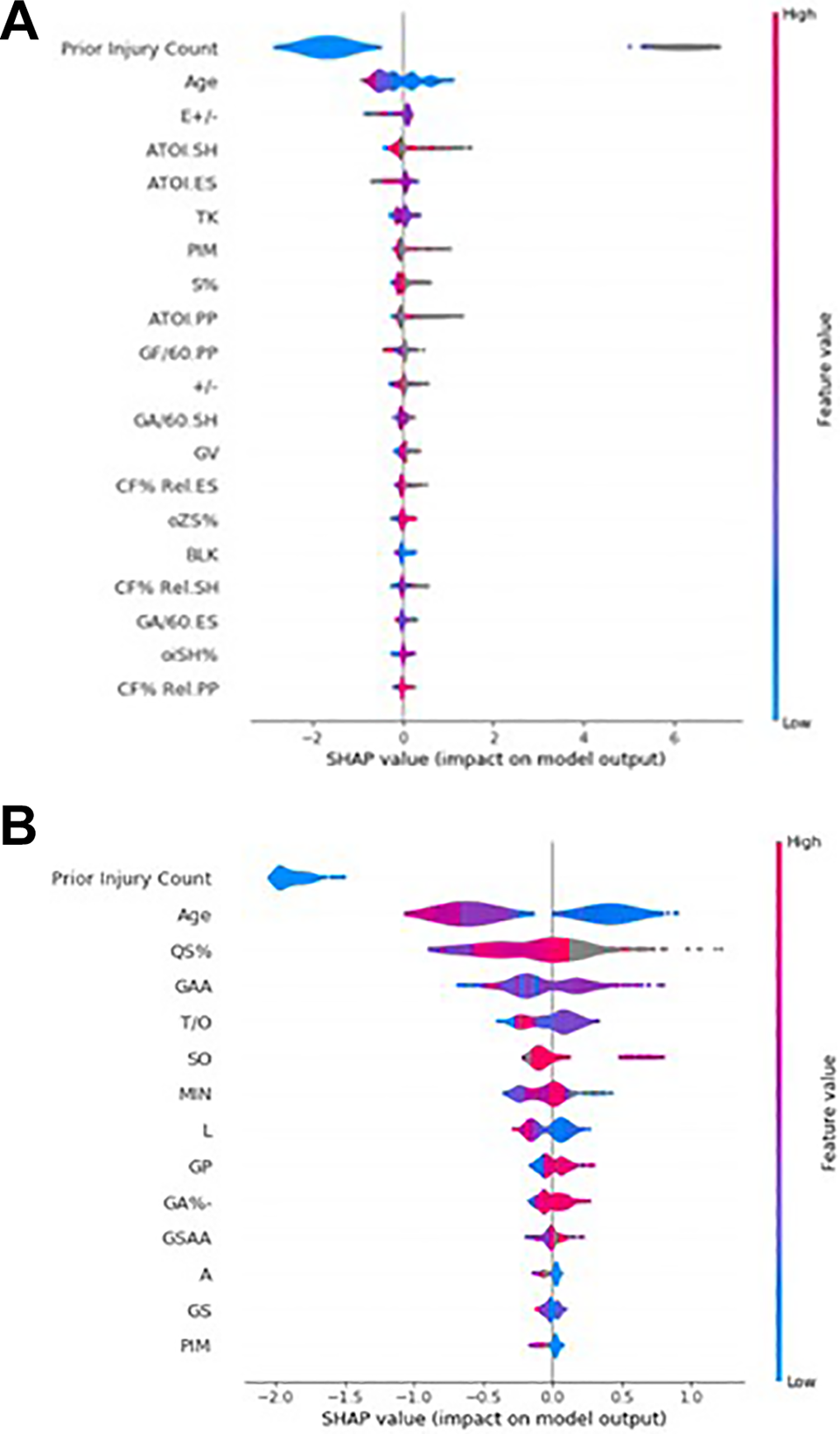
A summary Shapley Additive Explanations (SHAP) plot for National Hockey League goalies (A) and position players (B). The top 14 most important factors for model output are on the y axis. Factor impact on the model is on the x axis. For each factor, the distribution of values is displayed. A higher SHAP value indicates a factor that predicts higher injury probability, whereas a lower SHAP value indicates a factor that predicts a lower injury probability. Each datapoint is colored by the feature value. For example, age is colored blue for lower age values and red for higher age values.

Discussion

Historically, injury prevention for athletes was performed on a case-by-case basis, with the coaching and training staff working collaboratively to create training regimens and manage workloads for each individual athlete. As the implementation of “advanced analytics” in professional hockey begins to become standard across the NHL, teams must turn to new areas of potential improvement.⁷ We hypothesized that a machine learning algorithm, when applied to hockey players in the NHL, would be a powerful tool in injury risk assessment and prevention. Such an algorithm would provide an opportunity for team physicians and coaching staff to provide targeted preventive care, acutely manage player workloads, and potentially arbitrate contracts to reflect the value of availability.

From publicly available online resources, we compiled a comprehensive database detailing NHL player injury history, age, and 85 player performance metrics. From this database, we applied modern machine learning algorithms to create models capable of predicting next-season injury with good to excellent accuracy. For position players, XGBoost and Top 3 Ensemble provided improved performance over logistic regression. For goalies, only XGBoost provided improved performance over logistic regression. For both position players and goalies, the XGBoost algorithm provided the best performance, with excellent AUCs of 0.948 and 0.956, respectively. Based on SHAP analysis for both position players and goalies, prior injury count was the greatest predictor of future injury count (Figure 3). The superiority of machine learning in rudimentary predictive models suggests that regression analysis should not be the gold standard in injury prediction analytics.

Data science and the application of machine learning comprise a growing area of study that has already begun to revolutionize both industry and academia.¹⁸ As machine learning and artificial intelligence loom large over the field of medicine, doctors must learn not only to adjust but to improve. Although some physicians may be recalcitrant in accepting the integration of artificial intelligence into their practice, the impact that artificial intelligence will have on the field in the coming years is unarguable. Although physicians might not need to understand the theory or technical aspects involved in the construction of machine learning models, their practice of medicine would be greatly augmented by an ability to interpret the outputs of those models and communicate the risk of a given injury on the trajectory of an athlete’s career. Additionally, novel clinical inferences can be extracted from characteristics of the optimized model.

For example, imagine an orthopaedic surgeon working with a professional hockey team using the optimized model created in this study. From the model, the physician can receive an objective prediction of the level of injury risk for a given player, which can be used to guide course of care on a day-to-day basis as well as longitudinally throughout the season. Beyond providing individualized care, the physician can also analyze performance metrics and certain aspects of the model, such as the SHAP score, to better counsel their coaches and team general managers on injury prevention, team strategy, and player acquisition. For each variable used in the construction of the model, a SHAP score is calculated that effectively reflects the weight of that variable’s contribution in determining the output of the model. For example, suppose “Average time on ice per game while short-handed” (ATOI.SH) is found to be an important feature in the creation of the definitive injury prediction model. Coaches can then alter their rotations to prevent high-risk players from playing when the opposing team has a numerical advantage. Given the competitive nature of the sport, coaches might hesitate to not play their best players; however, machine learning can offer an objective evaluation of player-specific risk that may better inform coaches’ decision making in a long, grueling NHL season. Potential clinical insights such as this should incentivize physicians and physicians-in-training to familiarize themselves with the field of machine learning and data analysis.

This study is not without limitations. One such limitation was the lack of publicly accessible data surrounding the NHL. Many NHL teams hire teams of analysts that record custom, in-house metrics.^7,14 These metrics, which differ team by team, go far beyond the metrics available to the public. For example, certain teams are currently experimenting with puck and player tracking technology; others are contracting outside companies to track offensive zone time, in an attempt to assess player tendencies and possession quality.^2,20 Although our model was trained using >85 player metrics and was able to reach an excellent degree of accuracy in predicting future injury, the integration of a larger database of boutique statistics would only add to the predictive power and build upon all the model has already “learned” to correct and fine-tune predictions. One potential area of interest for future study could be the incorporation of specific player position (such as forward vs defense) in the assessment of future injury risk. Another limitation to our model is that all past injury history was considered equally, not accounting for degree of severity. A target of future study, given the acquisition of more explicit injury data, would be the assessment of degree of severity of past injury and its effect on future injury risk. Certainly, we expect more severe injuries to have a greater effect on future injury risk than minor ones; this remains a target of future model refinement.

Finally, the level of granularity of our data can be considered a limitation. Our injury data were often not specific; entries included phrases such as “upper limb injury” or “ankle injury.” As such, the clinical applicability is not readily deployable, as it depends on the existence of a centralized official injury database. Because of this ambiguity, we decided to include only prior injury count as a factor in the model, which is certainly unreliable and possibly clinically misleading without accounting for severity. The ability to incorporate more specific, graded injury data would present the opportunity for a more accurate next-season injury prediction model. Additionally, such data would allow the creation of new models that answer more complex questions beyond injury risk the subsequent season. One example would be a model that predicts the risk of a specific injury, such as the risk of a groin strain versus the risk of a stress fracture.

Conclusion

Advanced machine learning models such as XGBoost outperformed logistic regression and demonstrated good to excellent capability of predicting whether a publicly reportable injury is likely to occur the next season.

Footnotes

Final revision submitted April 9, 2020; accepted April 22, 2020.

One or more of the authors has declared the following potential conflicts of interest or source of funding: Internal funding for this study was provided by the Cleveland Clinic. M.S.S. has received educational support, consulting fees, and speaking fees from Arthrex. E.C.M. has received educational support from Pinnacle (Arthrex), consulting fees from Smith & Nephew, hospitality payments from Smith & Nephew and Stryker, and publishing royalties from Springer. B.U.N. has received educational support from Smith & Nephew and hospitality payments from Wright Medical and Zimmer Biomet. R.J.W. has received consulting fees from Arthrex. AOSSM checks author disclosures against the Open Payments Database (OPD). AOSSM has not conducted an independent investigation on the OPD and disclaims any liability or responsibility relating thereto.

Appendix

TABLE A2

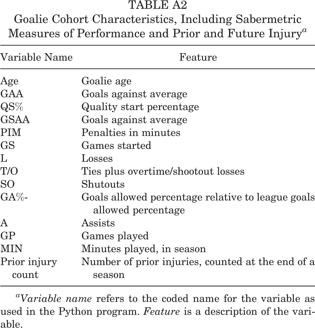
Goalie Cohort Characteristics, Including Sabermetric Measures of Performance and Prior and Future Injury ^a

Variable Name	Feature
Age	Goalie age
GAA	Goals against average
QS%	Quality start percentage
GSAA	Goals against average
PIM	Penalties in minutes
GS	Games started
L	Losses
T/O	Ties plus overtime/shootout losses
SO	Shutouts
GA%-	Goals allowed percentage relative to league goals allowed percentage
A	Assists
GP	Games played
MIN	Minutes played, in season
Prior injury count	Number of prior injuries, counted at the end of a season

^aVariable name refers to the coded name for the variable as used in the Python program. Feature is a description of the variable.

References

Ahmad

Dick

Snell

, et al. Major and Minor League Baseball hamstring injuries: epidemiologic findings from the Major League Baseball Injury Surveillance System. Am J Sports Med. 2014;42(6):1464–1470.

Barberio

. NHL analytics: why Moneyball will never work in professional hockey. Published 2019. Accessed October 24, 2019. https://puckprose.com/2019/05/03/moneyball-type-analytics-will-never-work-professional-hockey/

Beam

Kohane

. Big data and machine learning in health care. JAMA. 2018;319(13):1317–1318.

Belk

Marshall

McCarty

Kraeutler

. The effect of regular-season rest on playoff performance among players in the National Basketball Association. Orthop J Sports Med. 2017;5(10):2325967117729798.

Bini

. Artificial intelligence, machine learning, deep learning, and cognitive computing: what do these terms mean and how will they impact health care? J Arthroplasty. 2018;33(8):2358–2361.

Bond

Bennett

Noonan

. Evaluation of skating top speed, acceleration, and multiple repeated sprint speed ice hockey performance tests. J Strength Cond Res. 2018;32(8):2273–2283.

Castillo

. The NHL’s new tracking data introduces more ways for teams to get analytics wrong—defending big D. Published 2019. Accessed October 24, 2019. https://www.defendingbigd.com/2019/2/1/18203044/nhl-new-tracking-data-introduces-more-ways-for-teams-to-get-analytics-wrong-dallas-stars-fancy-stats

Chen

Guestrin

. XGBoost: a scalable tree boosting system. In: Balaji

, ed. Proceedings of the ACM SIGKDD International Conference on Knowledge Discovery and Data Mining. Association for Computing Machinery; 2016:785–794.

Cusimano

Ilie

Mullen

, et al. Aggression, violence and injury in Minor League Ice Hockey: avenues for prevention of injury. PLoS One. 2016;11(6):e0156683.

10.

Demers

. Riding a probabilistic support vector machine to the Stanley Cup. J Quant Anal Sport. 2015;11(4):205–218.

11.

Donaldson

Cusimano

. Economic burden of time lost due to injury in NHL hockey players. Inj Prev. 2014;20(5):347–349.

12.

Goutte

Gaussier

. A probabilistic interpretation of precision, recall and F-score, with implication for evaluation. Lecture Notes in Computer Science. 2005;3408:345–359.

13.

Foster

Shang

Wei

. A game-predicting expert system using big data and machine learning. Expert Syst Appl. 2019;130:293–305.

14.

Hascup

. Why NHL teams still view analytics as “state secret.” Published 2015. Accessed October 24, 2019. https://www.usatoday.com/story/sports/nhl/2015/02/19/advanced-stats-analytics-corsi-fenwick-shea-weber/23623373/

15.

Hernández-Orallo

Flach

Ferri

. Brier curves: a new cost-based visualisation of classifier performance. In: Proceedings of the 28th International Conference on Machine Learning, ICML 2011. 2011;585–592.

16.

Mosenthal

Kim

Holzshu

Hanypsiak

Athiviraham

. Common ice hockey injuries and treatment: a current concepts review. Curr Sports Med Rep. 2017;16(5):357–362.

17.

NHL stats, history, scores, & records. Accessed October 24, 2019. https://www.hockey-reference.com/

18.

Obermeyer

Emanuel

. Predicting the future-big data, machine learning, and clinical medicine. N Engl J Med. 2016;375(13):1216–1219.

19.

Pedregosa

Michel

Grisel

, et al. Scikit-learn: machine learning in Python. Accessed October 24, 2019. https://www.jmlr.org/papers/volume12/pedregosa11a/pedregosa11a.pdf

20.

Pope

. Blackhawks confident they’re leaders in NHL’s analytics movement, but puck-tracking revolution looms. Published August 17, 2019. Accessed October 24, 2019. https://chicago.suntimes.com/sports-saturday/2019/8/17/20805913/blackhawks-analytics-al-macisaac-andrew-thomas-nhl-statistics-contis-stan-bowman-corsi-seabrook

21.

ProSports Transactions. Professional hockey transactions archive. Accessed October 24, 2019. https://www.prosportstransactions.com/hockey/

22.

Reznik

Urish

. Understanding the impact of artificial intelligence on orthopaedic surgery. AAOSnow. September 2018.

23.

Schisterman

Perkins

Mumford

Ahrens

Mitchell

. Collinearity and causal diagrams: a lesson on the importance of model specification. Epidemiology. 2017;28(1):47–53.

24.

Scikit-learn: machine learning in Python—scikit-learn 0.21.3 documentation. Accessed October 24, 2019. https://scikit-learn.org/stable/whats_new/v0.21.html

25.

Seabold

Perktold

StatsModels: econometric and statistical modeling with Python. Published 2010. Accessed October 24, 2019. http://statsmodels.sourceforge.net/

26.

Simmons

Swedler

Kerr

. Injury surveillance of head, neck, and facial injuries in collegiate ice hockey players, 2009-2010 through 2013-2014 academic years. J Athl Train. 2017;52(8):776–784.

27.

Jazayeri

Lee

Khavanin

Dorafshar

Peacock

. Characterizing craniomaxillofacial injuries in American professional sports leagues. J Oral Maxillofac Surg. 2020;78(4):588–593.

28.

Youngstrom

. A primer on receiver operating characteristic analysis and diagnostic efficiency statistics for pediatric psychology: we are ready to ROC. J Pediatr Psychol. 2014;39(2):204–221.

Machine Learning Outperforms Logistic Regression Analysis to Predict Next-Season NHL Player Injury: An Analysis of 2322 Players From 2007 to 2017