
Abstract
In this study, we evaluate the performance of an encoder-decoder transformer and a Spatial–Temporal Graph Convolutional Network (GCN) architecture for basketball action classification using skeletal pose data. We isolate events of dribbling, passing, shooting, and rebounding throughout each basketball game and organize player joint frame windows to represent each activity. Analyzing 82 basketball games and over 400,000 events, we demonstrate that both architectures achieve high classification accuracy even if the number of tracked joints is significantly decreased. Our experiments confirm that reducing the full body skeleton from 16 joints per player to as few as 2 joints (left and right wrists) maintains robust performance while lowering computational costs and data storage requirements—a crucial consideration in high frame-rate basketball scenarios. These findings support a streamlined approach to pose-based action recognition that has the potential to enhance real-time decision making and deployment in sporting environments.
Keywords
Introduction
The relationship between referees and athletes is integral to the flow of professional sports, as referees’ decisions often shape critical moments and outcomes. Incorrect or biased referee decisions can significantly skew game results (Dohmen and Sauermann, 2016; Erikstad and Johansen, 2020). Recent advances in computer vision have led to the adoption of automated officiating of some aspects of professional sports such as baseball, soccer, and tennis to minimize human error (de Oliveira et al., 2023; Lee et al., 2024). Automated officiating has the potential to increase fairness and decision-making within sports. However, if not trained properly, these models can amplify biases and change gameplay dynamics (Leveaux, 2010; Thomas-Acaro and Meneses-Claudio, 2024).
Designing an effective automated officiating system requires the seamless integration of hardware and software infrastructure within a sporting facility. Professional basketball teams have already made substantial investments in data collection and analytics tools to support team initiatives (Wang et al., 2025). In contrast, our work explores increased technology investments at the overarching league level to support officiating use cases and accurate classification of gameplay events. A core hypothesis of this research is that by reducing the number of required input features and the volume of data collected, we can maintain high classification accuracy while enhancing overall system efficiency. This not only simplifies data collection, but also reduces computational costs, potentially enabling the use of more compact computing systems.
In this work, we explore using deep neural network models to better understand the relationship between the number of input features, data volume, and neural network model robustness. Through analyzing basketball pose data representing player joint positions during each frame of a game, we test the capability of various neural network architectures including a transformer encoder-decoder architecture and a Graph Convolutional Network (GCN) with Gated Recurrent Unit (GRU) temporal encodings to see if the models can accurately classify basketball activities including shooting, passing, rebounding, and dribbling.
Related Work
Prior research on skeletal-based action recognition has demonstrated the feasibility of classifying activities using joint-level data. However, many existing models rely on millions of parameters, Kinect sensors, and constrained environments often within single-agent settings (Song et al., 2020). Many action recognition studies have benchmarked model performance on the NTU RGB+D dataset (Shahroudy et al., 2016), one of the most widely used datasets for human action recognition with over 56,000 video samples (Shi et al., 2018). While extensive and valuable, NTU RGB+D primarily contains isolated actions performed by individuals in controlled lab settings, which do not reflect the complexity of real-world, multi-agent sports environments. For instance, Yan et al. developed a spatial-temporal GCN to classify activities like running using 18-joint skeletons from a Kinect sensor captured at 30 frames per second (fps) (Yan et al., 2018). Such approaches are computationally intensive, requiring additional hardware or extended compute times, which complicates live real-time deployment in professional sports environments.
In contrast, our work analyzes dynamic, live-game basketball pose data, featuring 10 concurrent skeletons (one per player), each with 29 joints tracked at 60 fps as players move throughout the court. This real-world, multi-agent environment is significantly more complex and less studied in prior work. We begin to address this by analyzing single-player activity classification by isolating one player skeleton out of all 10 skeletons per event. Additionally, we evaluate whether a reduced skeletal representation with less joints can maintain high classification accuracy, addressing the critical challenge of balancing efficiency and accuracy in real-time applications. The objective of this study is to evaluate variable joint classification accuracy which we demonstrate on one single skeleton, however this methodology can be expanded to multi-skeleton joint analysis. By developing a robust and scalable method for complex action recognition using minimal data input (no images), our approach addresses a pressing need in automated officiating and sports technology.
Experiment Methods
Data collection
The skeletal data is from the NBA Optical Tracking system, and the event annotations are from the NBA event feed across 82 games of the 2024–2025 NBA season. These datasets include skeletal pose data of 29 joints per player tracked at 60 frames per second (fps) and the event feed contains time occurrences of dribbles, passes, shots, and rebounds in each game. Overall, we gathered 274,530 events with 148,853 dribbles, 98,098 passes, 18,461 shots, and 9,118 rebounds.
While each individual event was not manually validated on a per-game basis, the optical tracking and event systems have been validated holistically by NBA personnel. Additionally, we manually validated a subset of events by visualizing 3D skeletal trajectories and confirming alignment with the associated event labels. For each event classification activity, we isolated a single player skeleton with 29 joints per frame and defined a 21 frame pose window as each of our classification tasks are dynamic and need to be defined over a sequence of frames rather than single frame classification. We selected a 21-frame window because, at 60 fps, this corresponds to approximately one-third of a second, which fully captures the skeletal joint movement during each event. The window size was determined after manually reviewing over 100 events, observing that the complete action typically occurs within this time span. The odd number of frames was chosen because the dataset flags a single timestamp for each event, and the window was centered around this flag as defined in Table 1.
Pose window definitions for each sequence type.
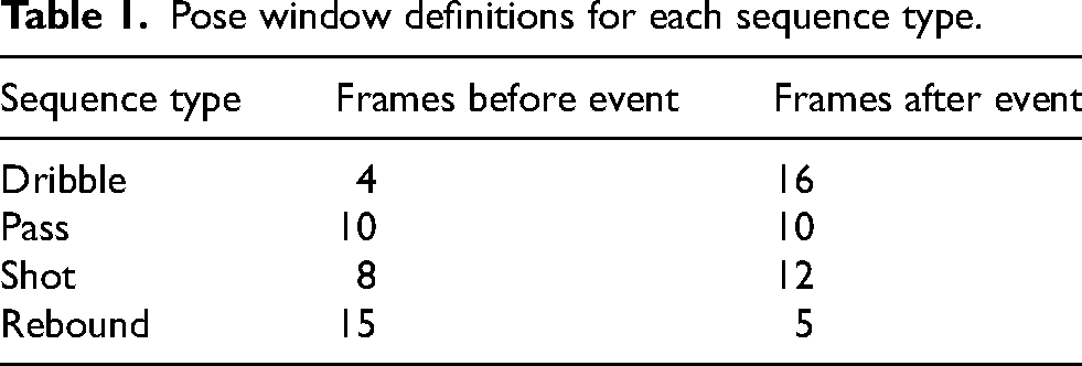
This difference in window frame selection per activity is due to the way the data provider flags each activity. Typically, shots and passes are defined immediately before the ball is released from the hand so we choose to capture more frames before the event flag to represent the entire duration of the event. Rebound event labels are the least consistent and are defined as the moment the ball touches a player’s hand after a missed shot attempt. As a result, the rebound events contain occurrences where a player jumps in the air to grab the ball and also moments where players are stationary.
The NBA Optical Tracking system is calibrated across multiple cameras per stadium and generates a stationary 3D global coordinate system. For each frame in the 21-frame window, player joints were identified with the
All 29 skeletal joints organized by body section.
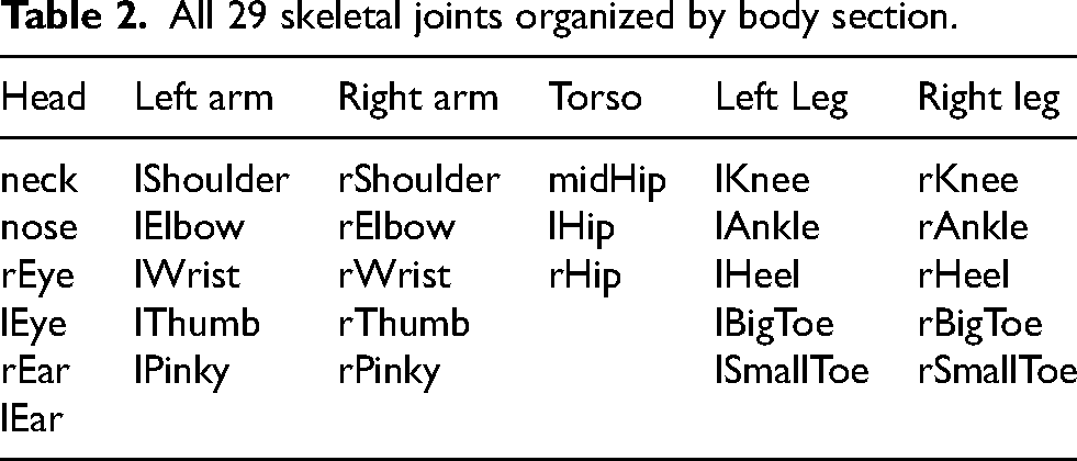
To simplify the scope of joint combinations, we restricted our analysis to a subset of 16 joints representing the human skeleton as shown in Figure 1.
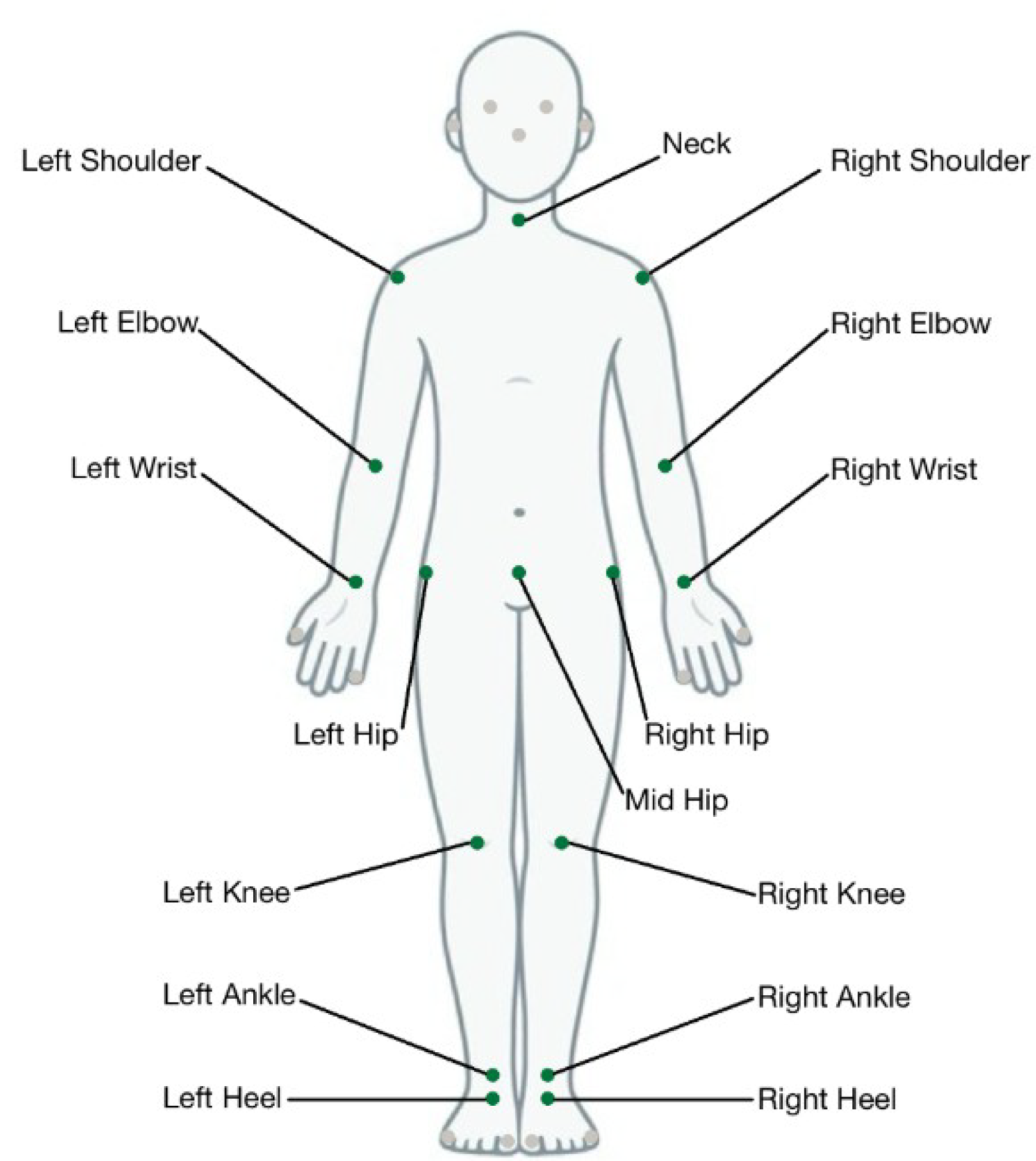
Top 16 joints selected for analysis.
Certain joint motions are indicative of specific basketball activities. For example, dribbling primarily involves upper body movement. More specifically, we expect the hands to exhibit significant motion across all activities, as the wrists are frequently engaged in interacting with the ball during dribbling, passing, shooting, and rebounding. To test how different parts of the body contribute to model performance, we organized the subset of 16 joints into 9 pairs, as outlined below:
Shoulder: [rShoulder, lShoulder] Elbow: [rElbow, lElbow] Wrist: [rWrist, lWrist] neck (singular): [neck] Knee: [rKnee, lKnee] Ankle: [rAnkle, lAnkle] Hip: [rHip, lHip] midHip (singular): [midHip] Heel: [rHeel, lHeel]
Even with this reduced subset, there are 511 total joint combinations as shown in Table 3. Each joint combination takes approximately 3 hours on average to train each model and complete hyperparameter tuning.
Total number of possible joint combinations.
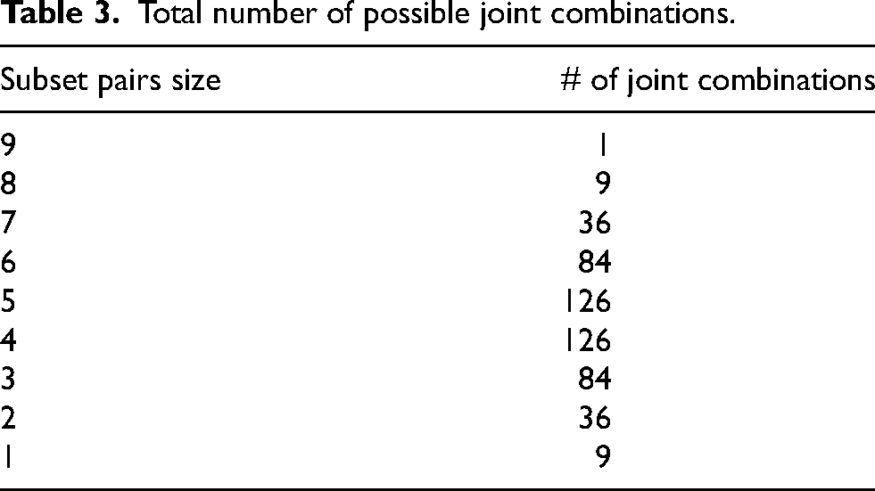
As opposed to testing all 511 joint combinations, we tested all 9-pair, 8-pair, 2-pair, and 1-pair combinations and then randomly selected 20 different combinations for each of the 3–7 pair configurations due to time constraints. To decide which joints to select, we analyzed the results from the 9, 8, 2, and 1 pair(s) experiments and assigned sampling weights to each joint pair based on their impact on the model’s overall classification accuracy. For example the elbow is twice as likely to be selected as the shoulder using this sampling algorithm. The resulting sampling weights are summarized in Table 4.
Joint sampling weights assigned based on empirical observations.

In total we tested 155 different joint combinations. The center of mass of each player during each frame was also added to our dataset before imputing into the model. A visualization of the player joint skeletons can be found at Figure 2

Tracked skeletal joints shown in a single frame from a basketball game.
Transformer model architecture
We explored two main architectural approaches for basketball action recognition from pose: a transformer based model using an encoder-decoder transformer architecture, and a Graph Convolutional Network which integrates GRU temporal encodings Figure 3.

GCN Diagram.
Our transformer projects per-frame joint and center of mass features to the model embedding dimension, adds a learnable positional encoding, and processes the sequence with encoder layers of multi-head self-attention. A minimal one-layer decoder with a single learnable query token attends over the encoder outputs to aggregate the sequence and the output is passed to a linear softmax head for classification.
The input to the transformer tensor can be represented as:
To enable the model to understand temporal order, we add a learnable positional encoding 
The transformer uses multi-head self-attention to compute interactions between each element in a sequence:
Each transformer layer is passed through a feedforward network to learn higher-level representations:
We include a minimal one-layer decoder that attends over the encoder outputs to aggregate the sequence. The final decoder output from the last transformer layer, 
Temporal GCN model architecture
Alternatively, the skeletal joint representation of our data can be analyzed as a graphical network. In this approach, we must keep track of the spatial-temporal relationship and can use a temporal graph convolution network (Yan et al., 2018). This model explicitly captures spatial and temporal dependencies, providing additional structural information for the classification tasks.
Our Graph Convolutional Network consists of four sequential GCN layers with ReLU activation and dropout, followed by temporal aggregation via a GRU layer. The final output of the GRU is passed through two fully connected layers with ReLU and dropout and the result is passed to a linear softmax head for classification.
The graph edge connectivity for spatial edges


At each GCN layer, node embeddings are updated as follows:
A temporal edge connection is used to propagate node features over time. We apply a Gated Recurrent Unit (GRU) to control the information update:
After processing multiple GCN layers, the node embeddings are aggregated using global mean pooling:
Similarly to the transformer, we pass our final layer through a fully connected softmax classification layer:
Graph construction and limb connectivity
For our GCN, the skeletal structure is modeled as a graph, where each node corresponds to a joint and edges represent limb connections as shown in Equation 6. For example when looking at our top 16 joints outlined in Figure 1, we defined the following limb pairs to capture the node connections most similar to the biomechanics of a human skeleton as outlined in Table 5. For each joint combination, we also define the limb connectivity pairs to input into the GCN.
Node connectivity defined for all 16 joints.

Experiment Setup and Training
We experimented with inputting our data into both model architectures outlined in the previous section. Our data was organized with separate labels per class.
Data augmentation
As described earlier, our initial event dataset is imbalanced with a significantly smaller number of shot and rebound events. To account for this, we mirrored our passes, shots, and rebound data points across the y axis by negating the x term. Since our dataset defines the center of court at (0,0) we are able to mirror events on the opposite side of the court by flipping x. After doing this our total number of events increased to 400,207 with 148,853 dribbles, 196,196 passes, 36,922 shots, and 18,236 rebounds. To account for the remaining imbalance we performed data augmentation by duplicating under-sampled classes and adding random noise to joint positions. This data augmentation technique was only applied to the training dataset. Our data was split into 60% train, 20% validation, and 20% test. The validation and test datasets were not augmented, only the training set. Due to mirroring across the x axis, the number of pass events exceeded the number of dribbles so we down sample passes to match the number of dribbles and up sample shots and rebounds to get a balanced training dataset size of 89,426 events per class.
Hyperparameter tuning
To perform hyperparameter tuning, we used Optuna, a hyperparameter optimization library to efficiently identify the best parameters per model instead of using a grid search. We applied Optuna across each joint configuration and data augmentation method. The parameters we looked to optimize for the transformer included Learning Rate (
For each joint combination, 20 Optuna trials were run with each study training 5 epochs to determine optimal weights. In each transformer trial, Optuna sampled from the following search space:
d_model: 256 n_head: 8 LR: 0.0007387 num_layers: 4 BS: 64
For the GCN model, the Optuna hyperparameters included LR, BS, Hidden Dimensions (
These hyperparameters were used to retrain each model over 15 epochs for final evaluation on withheld test set data.
Transformer model parameters
Across varying joint pair combinations and tuned hyperparameters, our encoder–decoder transformer model ranges from 0.86 million to 23.16 million learnable parameters. The smallest scenario occurs with a single joint (6 input features) where
GCN model parameters
Our GCN model including velocity and acceleration node feature dimensions ranges from 0.04 million to 0.63 million learnable parameters. The smallest scenario occurs with a singular joint and
Loss
To confirm our model was not overfitting we calculated the validation loss per epoch. As shown in Figure 4 the validation loss decreases over epochs and follows a similar trend to the training loss.

9 Pair Transformer Training vs Validation Loss (16 total joints).
Results
Transformer results
The transformer model performed well maintaining high accuracy with a reduced number of joints. When isolating a single joint pair, wrist performed the best (rWrist, lWrist) achieving 89.88

Transformer model per-activity accuracy compared to overall accuracy. Each point represents the accuracy for one particular set of joint pairs out of the 155 different combinations selected. The upper envelope represents the accuracy obtainable by the optimal set of joints. The results show that accuracy does not decrease significantly when removing certain joints.
Looking across every joint combination evaluated per pair, we tracked accuracy values and which joints were added or removed. We compared each 8 pair joint combination to all 7 pair combinations, each 7 pair to all 6 pair combinations and so forth. Using this method, we generated a marginal average impact graph that quantifies how removing each individual joint affects model accuracy as shown in Figure 6.
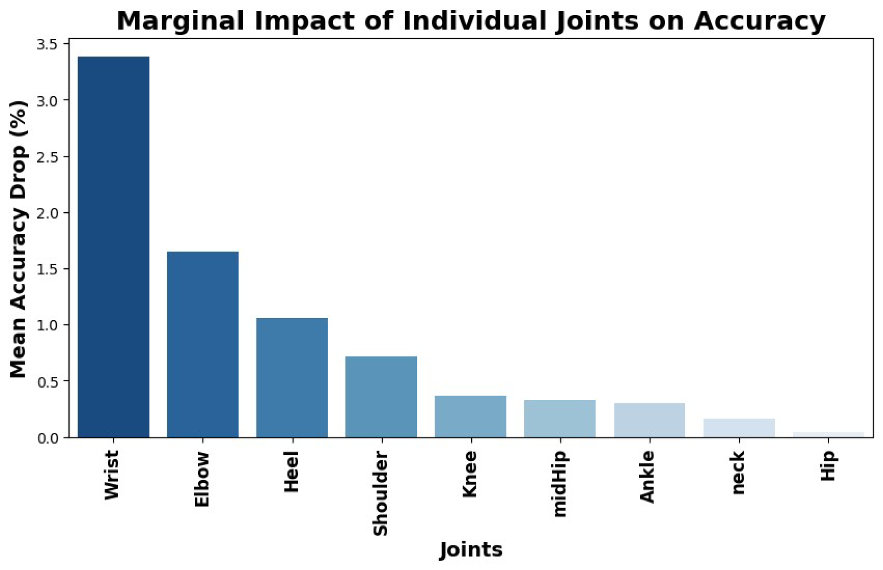
Marginal average impact of removing individual joints on model accuracy.
This analysis highlights that the wrist joints have the most significant effect on classification performance. In particular, when the wrist joints are removed, average marginal model accuracy decreases by 3.38
GCN results
After analyzing the results from the transformer, we took the top joint pairs and used the data to train our GCN model. For 3 pairs (6 joints), 2 different combinations were run: one set with [wrist, elbow, shoulder] and the other with [wrist, elbow, heel], to analyze the impact of including shoulder vs heel joints on our model. This time the model performed as expected and our GCN received a higher accuracy with the shoulder input of 92.81

GCN accuracy distribution with velocity and acceleration input. These represent the accuracies for the best joint pair choices. For example for 1 joint pair we show the accuracy for lWrist, rWrist.
Overall the best GCN configuration including velocity and acceleration achieved slightly higher accuracy than the best transformer pair using position alone. The GCN reached 93.64
To ensure a fair comparison with the transformer, which only receives position inputs, we also trained a version of the GCN using
The GCN takes in the spatial-temporal nature of joint data and we also had to establish the skeletal joint connections as outlined in the Temporal GCN Model Architecture section. For the skeletal joint connections, we assumed the closest joint connection to a biomechanical human skeletal joint connection would be most effective.
By accounting for the relationship between joints and between time steps our model is able to better predict each classification activity. Our best GCN model maintains high classification accuracy for dribbles, passes, and shots as shown in Figures 8 and 9. Rebound accuracy is lower at 83
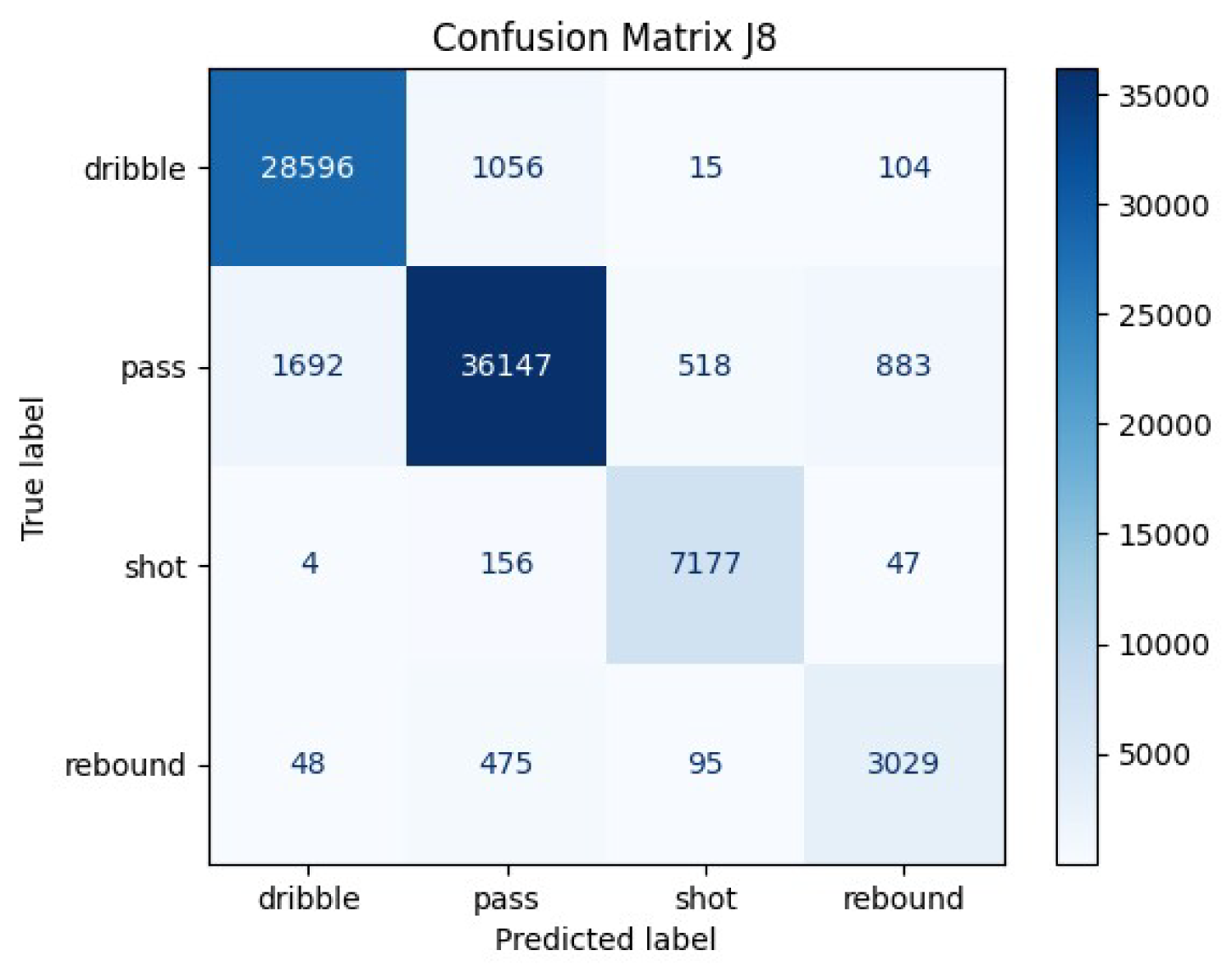
GCN 8 joint test set confusion matrix.

GCN 8 joint test set confusion matrix
KFold cross validation
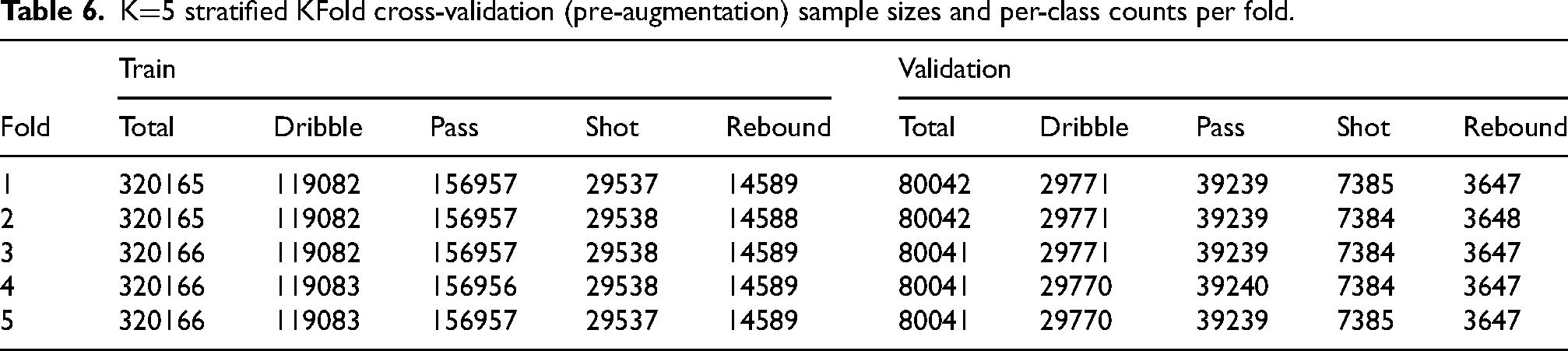
To ensure the validity of our model, we implemented stratified KFold cross validation which preserves the per-class activity proportions in every train and validation split such that each fold reflects the overall label distribution. Fold distribution sizes can be found in Table 6. For both the transformer and GCN we set
K
Our stratified KFold analysis confirms that our model achieves higher accuracy with using a reduced number of joints. For the transformer and both versions of the GCN, each achieved the highest mean overall accuracy using less than all joint pairs as shown in Figures 10–12. This result suggests that reducing the number of input joints can maintain high classification performance by removing joints with minimal or irrelevant motion. Since the basketball activities we focused on, such as dribbling, passing, shooting, and rebounding, primarily involve upper body motion, retaining only the most active joints (e.g., wrists and elbows) enables the models to more effectively focus on the most informative movements.

Stratified KFold Transformer Results. Vertical bars represent 95

Stratified KFold GCN Results with pose data input. Vertical bars represent 95

Stratified KFold GCN Results with enhanced velocity and acceleration input. Vertical bars represent 95
We observed that the GCN with velocity and acceleration inputs had the most stable performance across folds, with the highest standard deviation of only 0.38
Conclusion
Overall, we were able to achieve high classification accuracy on both our encoder-decoder transformer and GCN with GRU temporal encoding architectures. Through analyzing 82 games and 400,000 events, we were able to generate a converging loss and validated our data was not overfitting to training data, and confirmed trends with stratified KFold cross validation.
Our results successfully show for both models that high model accuracy can be maintained while significantly reducing the number of joints. In a basketball game, efficiency is crucial and by reducing the computational load from tracking 10 players at 60 fps for 29 joints per player to potentially just 2 joints (rWrist and lWrist) will allow for reduced compute cost and data storage. This reduction will allow for faster model deployment and has the potential to provide officiators with necessary information to improve decisions. We can confirm with both methods that joint selection impacts model performance for both methods suggesting that an accurate and efficient classification with a reduced skeleton is possible.
Future Work
Due to limited processing cycles, we were unable to exhaustively train models on every possible joint combination from 1 to 29 joints. Future work could focus on identifying the exact optimal joint configurations for each classification task. Additionally, since the number of rebound and shot events in the dataset was significantly lower compared to dribble and pass activities, it would be valuable to collect more examples of these underrepresented classes. Further, rebounds could potentially be subdivided into two categories for when a player jumps for a rebound vs non-jumping rebounds. This paper focused on single skeleton activity classification however, the methods can also be extended to analyze multi-player skeleton activities including pick and rolls. In our GCN, we only selected joint connections most similar to the biomechanics of human skeletal joints. Future studies could investigate alternative connectivity patterns, including many-to-one connections, and experiment with longer time windows. Using 60 fps cameras, a 21 frame event window (about 1/3 of a second) may not be the most optimal time window to capture these activities. Finally, analyzing which events are consistently misclassified, such as the ambiguous cases between pump fake shots and passes, could provide insights into the limitations of current models and guide further improvements.
Footnotes
Ethical Considerations
All data was provided from a 3rd party source and no identifying characteristics were used to train or evaluate the model.
Funding
The authors disclosed receipt of the following financial support for the research, authorship, and/or publication of this article: This project was supported by the NBA through the MIT Sports Lab Pro Sports Consortium.
Declaration of Conflicting Interests
The authors declared no potential conflicts of interest with respect to the research, authorship, and publication of this article.
Data Availability
The data is the property of the NBA. Researchers interested in access to the data may contact Greg Cartagena at gcartagena@nba.com.
Data and Code Availability
Appendix
GCN precision, recall, and F1 accuracy results for each joint pair excluding velocity and acceleration data. TP

| Pairs | # Joints Used | Class | TP | FP | FN | Precision | Recall | F1 |
|---|---|---|---|---|---|---|---|---|
| 1 | 2 | Dribble | 27393 | 3965 | 2378 | 0.8736 | 0.9201 | 0.8962 |
| 1 | 2 | Pass | 29564 | 2841 | 9676 | 0.9123 | 0.7534 | 0.8253 |
| 1 | 2 | Shot | 5714 | 688 | 1670 | 0.8925 | 0.7738 | 0.8290 |
| 1 | 2 | Rebound | 3066 | 6811 | 581 | 0.3104 | 0.8407 | 0.4534 |
| 2 | 4 | Dribble | 27389 | 2145 | 2382 | 0.9274 | 0.9200 | 0.9237 |
| 2 | 4 | Pass | 33829 | 2984 | 5411 | 0.9189 | 0.8621 | 0.8896 |
| 2 | 4 | Shot | 6689 | 1060 | 695 | 0.8632 | 0.9059 | 0.8840 |
| 2 | 4 | Rebound | 2685 | 3261 | 962 | 0.4516 | 0.7362 | 0.5598 |
| 3 | 6 | Dribble | 27388 | 2063 | 2383 | 0.9300 | 0.9200 | 0.9249 |
| 3 | 6 | Pass | 35281 | 7039 | 3959 | 0.8337 | 0.8991 | 0.8652 |
| 3 | 6 | Shot | 3419 | 322 | 3965 | 0.9139 | 0.4630 | 0.6147 |
| 3 | 6 | Rebound | 2054 | 2476 | 1593 | 0.4534 | 0.5632 | 0.5024 |
| 3 | 6 | Dribble | 27747 | 2162 | 2024 | 0.9277 | 0.9320 | 0.9299 |
| 3 | 6 | Pass | 32877 | 2041 | 6363 | 0.9415 | 0.8378 | 0.8867 |
| 3 | 6 | Shot | 6911 | 857 | 473 | 0.8897 | 0.9359 | 0.9122 |
| 3 | 6 | Rebound | 3156 | 3984 | 491 | 0.4420 | 0.8654 | 0.5851 |
| 4 | 8 | Dribble | 27383 | 1804 | 2388 | 0.9382 | 0.9198 | 0.9289 |
| 4 | 8 | Pass | 34231 | 2919 | 5009 | 0.9214 | 0.8723 | 0.8962 |
| 4 | 8 | Shot | 6410 | 395 | 974 | 0.9420 | 0.8681 | 0.9035 |
| 4 | 8 | Rebound | 3115 | 3785 | 532 | 0.4514 | 0.8541 | 0.5907 |
| 5 | 10 | Dribble | 27209 | 2261 | 2562 | 0.9233 | 0.9139 | 0.9186 |
| 5 | 10 | Pass | 31818 | 4153 | 7422 | 0.8845 | 0.8109 | 0.8461 |
| 5 | 10 | Shot | 5817 | 628 | 1567 | 0.9026 | 0.7878 | 0.8413 |
| 5 | 10 | Rebound | 2647 | 5509 | 1000 | 0.3245 | 0.7258 | 0.4485 |
| 6 | 11 | Dribble | 26953 | 2604 | 2818 | 0.9119 | 0.9053 | 0.9086 |
| 6 | 11 | Pass | 33886 | 4764 | 5354 | 0.8767 | 0.8636 | 0.8701 |
| 6 | 11 | Shot | 5540 | 869 | 1844 | 0.8644 | 0.7503 | 0.8033 |
| 6 | 11 | Rebound | 2441 | 2985 | 1206 | 0.4499 | 0.6693 | 0.5381 |
| 7 | 12 | Dribble | 27949 | 3182 | 1822 | 0.8978 | 0.9388 | 0.9178 |
| 7 | 12 | Pass | 33175 | 2726 | 6065 | 0.9241 | 0.8454 | 0.8830 |
| 7 | 12 | Shot | 6530 | 600 | 854 | 0.9158 | 0.8843 | 0.8998 |
| 7 | 12 | Rebound | 2746 | 3134 | 901 | 0.4670 | 0.7529 | 0.5765 |
| 8 | 14 | Dribble | 27244 | 3949 | 2527 | 0.8734 | 0.9151 | 0.8938 |
| 8 | 14 | Pass | 33107 | 3574 | 6133 | 0.9026 | 0.8437 | 0.8721 |
| 8 | 14 | Shot | 6438 | 816 | 946 | 0.8875 | 0.8719 | 0.8796 |
| 8 | 14 | Rebound | 2404 | 2510 | 1243 | 0.4892 | 0.6592 | 0.5616 |
| 9 | 16 | Dribble | 26409 | 3848 | 3362 | 0.8728 | 0.8871 | 0.8799 |
| 9 | 16 | Pass | 31069 | 3403 | 8171 | 0.9013 | 0.7918 | 0.8430 |
| 9 | 16 | Shot | 6893 | 1350 | 491 | 0.8362 | 0.9335 | 0.8822 |
| 9 | 16 | Rebound | 2599 | 4471 | 1048 | 0.3676 | 0.7126 | 0.4850 |