Sage Journals: Discover world-class research

Abstract

The evaluation of player performance is an important topic in sports analytics and is used for team management, scouting, and in sports broadcasts. When evaluating the performance of ice hockey players, many metrics are used, including traditional metrics such as goals, assists, and points and more recent metrics such as Corsi and expected goals. One weakness of such metrics is that they do not consider the context in which the value for the metric was assigned. Other advanced metrics have been introduced, but as they are not easily explainable to practitioners, they may not make it into the hockey discourse. In this paper we introduce new goal-based metrics that (i) are based on traditional, well-known metrics, and thus easily understandable, (ii) take context into account in the form of time, manpower differential, and goal differential and (iii) add a new aspect by taking into account the importance of goals regarding their contribution to team wins and ties. We describe the intuitions behind the metrics, give formal definitions, evaluate the metrics and show correlations to the traditional metrics. We have used data from seven NHL seasons and show which players stand out with respect to the number of goals and the importance of goals.

Keywords

sports analytics ice hockey performance Metrics

Introduction

Sports analytics is a field that has increased in popularity in recent years. One particular component of sports analytics that has seen a large increase in research is performance evaluation, both for teams and players, as it provides more insight into how we view and value the aspects of a sport. In team sports, such as ice hockey, soccer, and basketball, team performance can be analyzed from the perspective of team success, e.g., wins and total points earned. For player performance, the emphasis is instead on how an individual player contributes to the team (Singh, 2020).

The metrics used for evaluating performance have also changed drastically over time. Historically, the most available and basic statistics have been used to evaluate and compare players (Nandakumar and Jensen, 2019). In ice hockey, metrics such as goals, assists, points, and $+ / -$ have been used, whereas basketball has points, rebounds, assists, blocks, and steals, and soccer has goals and assists. A critique of these basic metrics is that they do not take context into account. Many new performance metrics, some introducing context, have been proposed for a more comprehensive evaluation. Examples include expected threat and the VAEP (valuing actions for estimating probabilities) framework for soccer (Decroos et al., 2019), player efficiency rating, game score and win shares for basketball (Sarlis and Tjortjis, 2020), while ice hockey has point shares and game score (Nandakumar and Jensen, 2019). Although many of these metrics provide new insights, they need to be explainable to hockey staff to be used.

Although some metrics take context into account for goals, e.g., the location of the shot, few consider the importance of goals. For instance, a goal scored when the team is in the lead with 5–0 at the end of the game, is most likely not crucial for winning. In contrast, scoring a goal when the score is tied at 1–1 with some seconds left of the game, is of more importance for winning. Furthermore, some players have a reputation for often scoring important goals, while others may have a reputation for mainly scoring when the team is playing ‘easier’ games. For instance, during the 2013-2014 season the Washington Capitals’ Alexander Ovechkin ranked the highest regarding game-tying and lead-taking goals while he only ranked 29 $^{th}$ regarding goals scored when the team is already in the lead.

In this paper, our aim is to introduce new goal-based metrics for evaluating the performance of ice hockey players. The metrics should take into account context and provide new insights. For this work we have chosen to focus on the importance of goals in the sense of having important contributions to winning or tying games. Further, the metrics should be easily understandable and based on well-known traditional metrics. To achieve these goals, we introduce the notion of goal importance. We introduce variants of the traditional goals (G), points (P),¹ assists (A) and $+ / -$ metrics that take into account the importance of the goals. By accounting for the importance of each goal, compared to these traditional metrics, our metrics better capture how much each player’s goals, assists, or on-ice presence may have contributed to a positive game outcome (e.g., by scoring game-deciding goals) and give less weight to players that score most of their goals when the outcome of a game may already be decided. Further, we can use the average importance of goals related to traditional metrics as metrics on their own. By introducing these metrics we are able to look at player performance related to goals in different complementary ways: the traditional metrics, the new variants that take into account the importance of the goals in which a player is involved, and the metrics measuring the average importance of the goals in which a player is involved for a particular traditional metric.

The paper is organized as follows. In Section ‘Related work - measuring performance in ice hockey’ we discuss previous work on measuring performance of players and player pairs in ice hockey. Then, we discuss a method for defining a new metric in Section ‘Defining a metric’ and the data we use in Section ‘Data’. We follow the different steps in the method by showing the intuition behind the metric (Section ‘Intuition behind metric’), and defining the importance of goals and the new metrics for the regular season (Section ‘Metrics definition’). We evaluate the metrics using the eye test (Section ‘Eye test for GPIV metrics’), and by computing the correlations between the new metrics and traditional metrics (Section ‘Correlations of GPIV metrics with traditional metrics’ and appendix A). We also look at whether data from an ongoing season can be used to predict the end-of-season values for the new metrics in Section ‘Prediction of GPIV metrics’. Finally, we show how our approach can be used to evaluate performance of player pairs (Section ‘Player pairs’). The paper concludes in Section ‘Conclusion’. In the appendix we discuss issues related to the stability of the metrics over different seasons (appendix B), whether we can use data from previous seasons, and if so, how much data, to compute an approximation of the metrics for an ongoing season (appendix C), and give results for the playoffs (appendix D).

Related work - measuring performance in ice hockey

When evaluating the performance of ice hockey players, it is most common to use metrics that attribute a value to the actions the player performs (e.g., scoring a goal for the goals metric or giving a pass that leads to a goal for the assists metric) and then compute a sum over all those actions. Some extensions to these traditional metrics have been proposed, e.g., for the $+ / -$ metric using regularized logistic regression models (Macdonald, 2011; Gramacy et al., 2013). There is also work on combining metrics, such as in Gu et al. (2019) where principal component analysis is used on 18 basic stats. Some of the approaches for player performance metrics take game context into account such as event impacts. For instance, in Schuckers and Curro (2013) the impact of each event is determined by the probability that it leads to a goal in the subsequent 20 seconds. Other works model the dynamics of an ice hockey game using Markov games where two opposing sides (i.e., the home team and the away team) try to reach states in which they are rewarded (e.g., scoring a goal) (Thomas et al., 2013; Kaplan et al., 2014; Routley and Schulte, 2015; Schulte et al., 2017a, 2017; Liu and Schulte, 2018; Sans Fuentes et al., 2019; Ljung et al., 2019). One critique of these more advanced metrics is that they are not easily understandable by or explainable to practitioners such as coaches, players, and GMs. An approach to predict the tier (e.g., top 10%, 25%, or 50%) to which a player belongs is presented in Lehmus Persson et al. (2020).

The importance of scoring the first goal in the NHL is investigated in Brimberg and Hurley (2009), where it is reported that the win probability is approximately 70% if the first goal is scored in the first period. This analysis assumes an equal win probability at the start of the game. The importance of a two-goal lead is analyzed in Brimberg and Hurley (2012) while Gill (2000) examines late-game reversals. Teams who have taken a two-goal lead win in 83% of games, while having the lead after two periods leads to a win in 84% and 80% of games for the home and away team, respectively. The work most similar in spirit to our work in taking the importance of goals into account is (Pettigrew, 2015), where first a probability is computed for the home team winning the game (but not tying the game as we do). The probability takes into account the remaining time in the game, the goal differential and the manpower differential. It is then used for introducing the added goal value metric for a player. This metric measures the difference between the change in win probability that occurred from each of the player’s goals (similar to the GPIV we introduce in Section ‘Defining an importance value’), and the expected change in win probability based on league average. In our work, we additionally use such a metric to define variants of traditional metrics.

We note that the introduction of new metrics may change the way the game is played. For instance, in Johansson et al. (2022) it was shown that team play transitioned first to taking more shots (high Corsi, shot-based), and then to taking high-quality shots (high expected goals). This point is also highlighted in Nandakumar and Jensen (2019), and similar trends have also been observed in, e.g., soccer (Van Roy et al., 2021).

New metrics can also be used ‘behind the scenes’, where coaches, managers, and GMs may use data-driven approaches for decision-making. An analytical approach has been proven successful for NBA, NFL, and MLB teams as they were able to select players with a far greater future value than the players selected prior. However, the analytical approaches present in, e.g., the NBA and NFL are less utilized in ice hockey, leaving a knowledge gap of what impacts the value of a prospect (Farah and Baker, 2020; Tingling, 2017). One way to increase this knowledge is the development of new methods and metrics to evaluate players. In Chaikof et al. (2022), an automatic scouting framework is proposed to identify player habits and possible developmental areas, which may be a time-consuming task. It has also been reported in Farah and Baker (2021) that drafting well in the NHL is only accurate for the first two rounds, leaving the remaining five rounds as more of a gamble. Due to the salary structure of the NHL, where entry-level contracts given to drafted players can have a monetary value far less than the production a player provides, drafting the correct player may be the difference between success and failure (Nandakumar and Jensen, 2019). Performance metrics applicable to potential draftees can thus also impact the way decisions are made, and recent work by Kumagai et al. (2022) presents one method for predicting the estimated ability of prospects and illustrates how it can be used to construct a draft ranking.

As ice hockey is a team sport, it is not enough to only look at the performance of individual players. Lineup management, for instance, can benefit from identifying pairs of players that perform well when sharing the ice. One of the most frequent metrics for determining what happened when a player was on the ice is $+ / -$ . However, the metric is typically criticized due to its disregard of contextual information (Thomas et al., 2013). Alternative approaches have been, e.g., regularized logistic regression for predicting player impact on scoring (Gramacy et al., 2013) and Cox proportional hazards models for the goal-scoring processes of the home and away team (Thomas et al., 2013). In both of these studies, the results are also generalized to player pairs. In Gramacy et al. (2013) only four player pairs were found to have a significant impact on team success with the player pair of David Krejci and Dennis Wideman having a high negative impact while the pair of Joe Thornton and Patrick Marleau had a positive effect on their team for the seasons between 2007-2008 and 2010-2011. Similarly, Thomas et al. (2013) analyzes the additional impact playing alongside another player has for a given player between 2007-2008 and 2011-2012. It is reported that pairing Patrice Bergeron and Brad Marchand is beneficial, while playing Sidney Crosby alongside Evgeni Malkin may be more detrimental. In Ljung et al. (2019) the work of Routley and Schulte (2015) is extended to take into account pairs of players. The metrics are based on actions when both players in the pair are on the ice. The results in these papers, do, however, not account for the importance of goals. In other sports, such as soccer, studies have also attempted to quantify the chemistry between a pair of players and how their joint performance impacts the offensive and defensive quality of their team Bransen and Van Haaren (2020).

Defining a metric

When defining a metric, several questions must be addressed. First, there are some questions regarding the purpose of the metric and its definition.

What are the intuitions behind the metric? It is important to know why a new metric is introduced. Usually, interesting observations regarding the game, that are not addressed by existing metrics, lie at the base of introducing new metrics. Therefore, a new metric should measure something that is not already measured by other metrics.

How is the metric defined? Once the intuitions and purpose of the new metric are clear, a formal definition of the metric is needed that allows us to compute the values for the metric.

Further, we need to evaluate the metric. This is not a simple task as we usually do not have a gold standard against which to evaluate. Therefore, the metric’s behavior is usually considered from different points of view, including passing the eye test, finding correlations with existing metrics, and looking at a metric over different seasons.

Does the metric pass the eye test? Although there is no gold standard, based on the intuitions behind the metric, experts may expect a certain ranking of the players based on the new metric. The eye test checks whether the actual ranking according to the new metric makes sense according to the expectations of the experts.

Are there correlations with existing metrics? A perfect correlation to existing metrics would mean that these metrics essentially measure the same thing. This could be interesting as an insight or in the case that it is easier to measure the new metric than existing metrics. However, as the intuitions behind the new metric usually deal with aspects that were not taken into account by existing metrics, there will not be a perfect correlation and this is what we would want. However, it is still interesting to check the correlation between the new metric and well-established metrics. A high correlation would show that the metric behaves in a similar way to a well-established metric, but still brings something new.

Is the metric stable? The values for metrics will differ from each other over different seasons. However, unless for good reasons, they should not change too drastically.

Finally, it is interesting to look at whether the value of the metric can be predicted.

Can one predict the value of the metric at the end of a season based on data for part of the season? For some traditional metrics the value of a metric after half of the season gives a good indication of the value at the end of the season. Therefore, it is interesting to check whether data for part of the season would allow predicting the value of the metric at the end of the season.

Data

We have used play-by-play data from the NHL, seasons 2007-2008 to 2013-2014. The data was generated for the work in Routley and Schulte (2015). It is available at https://www2.cs.sfu.ca/∼oschulte/sports/.

Intuition behind metric

The observations on which our new metrics are based are the following. First, we investigated when goals are scored. We did this for different time intervals from seconds to minutes. Figure 1 shows the results of goals per minute for the 2013-2014 season and this is representative of all seasons and most time intervals. We note that few goals are scored in the first minute of the game. Further, during the last minute of the game, at least three times as many goals are scored than for any other minute in the game. A possible explanation is the higher frequency of 6 on 5 situations at this time of the game, in which a team’s gamble to pull their goaltender often results in either them scoring a goal (in part helped by their extra attacker) or the other team scoring an empty-net goal. We also note that power-plays more often result in goals and that shorthanded goals are not that common. A team’s strategy may also shift depending on the current score. Our metrics, therefore, take time, goal differential, and manpower differential into account.

Figure 1.

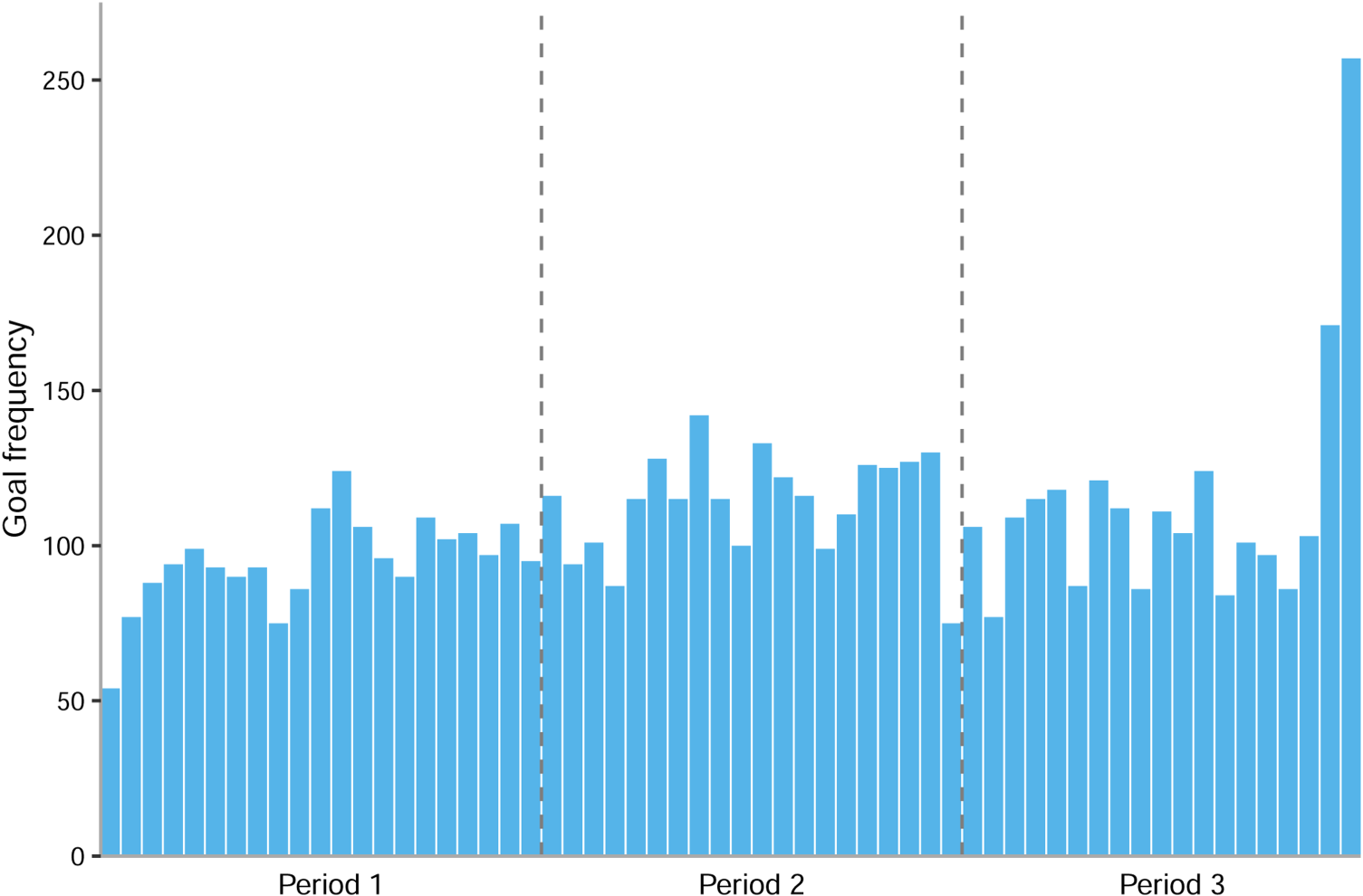
Goal frequency for each minute of regulation time in the NHL during the 2013-2014 regular season.

Another observation is that not all goals are equally important for producing game points, i.e., 2 PTS for a win, 1 PTS for an overtime loss, and 0 PTS for a regular time loss in the NHL. For instance, scoring the 6th goal for the team when already leading 5-0, will most likely not be contributing much to obtaining 2 PTS. The team would most likely win anyhow. However, a goal that ties the game in the last second of the game normally secures 1 PTS (while just before the goal the team would have 0 PTS) and therefore is an important goal. Our new metrics take the importance of a goal for producing PTS into account.

Metrics definition - GPIV-weighted performance metrics

In this section, we define our new metrics. The game outcomes are different for the regular season (win, overtime loss, regulation time loss earning 2, 1, and 0 PTS respectively) and the playoffs (win or loss in best-of-seven format). In this section we focus on the regular season. Playoffs are discussed in the appendix D.

Game Points Importance Value (GPIV) - regular season

Defining an importance value

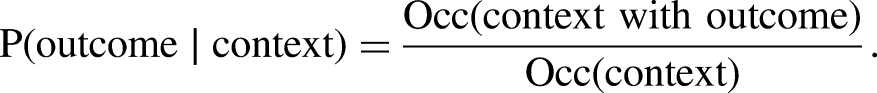
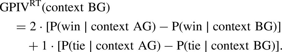
As a basis for our new metrics, we need to formally define the importance of a goal. Our intuition is that the importance of the goal represents the change in the probability of the team taking points for the game (PTS) before and after the goal has been scored.² Further, as discussed earlier, we take into account time (t) for which we choose one-second intervals, goal differential (GD), and manpower differential (MD). This we call a context.³

We next define the probability of an outcome of a game given a context. For regulation time, the outcome of a game can be a win, a tie⁴ and a (regulation time) loss. For overtime, the outcome of a game is an overtime win or an overtime loss. We define the probability of an outcome of a game given a context, as the ratio of the number of occurrences of the context that have resulted in the outcome and the total number of occurrences of the context in our dataset:

P (outcome ∣ context) = \frac{Occ (context with outcome)}{Occ (context)} .

We then attribute a Game Points Importance Value (GPIV) to a context. Intuitively, the GPIV represents how much a goal in a particular context increases or decreases the expected game points. For regulation time, a win earns the team 2 PTS, a tie 1 PTS, and a loss 0 PTS. For overtime, the winning team earns an additional 1 PTS (i.e., in addition to the 1 PTS for the tie), while the losing team does not earn any additional PTS.

In regulation time, when a goal is scored, the context after the goal (context AG) has the same time as the context before the goal (context BG), but the GD is changed by one and the MD may (minor penalty power-play goal) or may not change (even strength, short-handed, or major penalty power-play goal). Based on this intuition, we define the GPIV for regulation time in the NHL as follows:

\begin{aligned} {GPIV}^{RT} (context BG) \\ = 2 \cdot [P (win ∣ context AG) - P (win ∣ context BG)] \\ + 1 \cdot [P (tie ∣ context AG) - P (tie ∣ context BG)] . \end{aligned}

In overtime, when a goal is scored, the game ends and the additional PTS is awarded. On average, teams have an equal probability to earn the extra point. The probability of a win before the goal is, thus, 0.5. For the goal-scoring team, the probability of winning the game when the goal is scored becomes 1. The GPIV of the goal, representing the difference in expected game points, is therefore 0.5 for overtime goals:

{GPIV}^{OT} (context BG) = 0.5.

GPIV with accounting for rare goals in regulation time

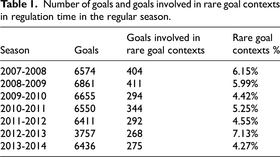
As the robustness and quality of the computed GPIV for regulation time depends on the number of occurrences of the context, some consideration should be given to goal contexts that are deemed rare. In general, when the number of occurrences of a context increases, the impact of an individual occurrence on GPIV decreases. In this paper, we define a rare goal context as a goal context that has less than ten occurrences across all three possible outcomes for regulation time (i.e., win, tie, or loss), for the state before and/or after the goal.

The choice of ten occurrences was motivated by a noticeable decrease in the point-wise variance of GPIV for goal contexts that had ten or more occurrences, compared to those that had fewer occurrences. Most rare goal contexts occur when GD is large ( $\leq - 4$ or $\geq 4$ ) and/or MD is $- 2$ or $2$ . For these rare goal contexts, the GPIV is volatile and can result in extreme values ( $\leq - 1.5$ or $\geq 1.5$ ). We also note that contexts with MD = 2 or MD = $-$ 2 have the highest variance, which can be explained by the fact that these contexts do not occur as often as the other contexts, and at least for MD = $- 2$ , goals are rarely scored.

In Table 1 we show the number of occurrences of goals involved in rare goal contexts according to our definition. For instance, in the 2013-2014 season 275 of the 6436 regulation-time goals, i.e., approximately 4.27%, were involved in rare goal contexts. Among these goals, 133 had a rare before-goal context, 90 had a rare after-goal context, and 52 had both a rare before-goal context and a rare after-goal context.

Table 1.

Number of goals and goals involved in rare goal contexts in regulation time in the regular season.

	Goals	Goals involved in	Rare goal
Season	Goals	rare goal contexts	contexts %
2007-2008	6574	404	6.15%
2008-2009	6861	411	5.99%
2009-2010	6655	294	4.42%
2010-2011	6550	344	5.25%
2011-2012	6411	292	4.55%
2012-2013	3757	268	7.13%
2013-2014	6436	275	4.27%

To mitigate the volatility of these rare goal contexts, we raise the number of occurrences of these contexts in an artificial way by taking into account the neighboring contexts and their occurrences. A neighboring context of a given context is a context that is close in time, GD, and MD to the given context. Formally, we use a weighted Manhattan distance to account for the different units in time, GD, and MD. We define the distance between context (t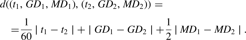 $_{1}$ ,GD $_{1}$ ,MD $_{1}$ ) and (t $_{2}$ ,GD $_{2}$ ,MD $_{2}$ ) as follows:

\begin{aligned} d ((t_{1}, G D_{1}, M D_{1}), (t_{2}, G D_{2}, M D_{2})) \\ = \frac{1}{60} ∣ t_{1} - t_{2} ∣ + ∣ G D_{1} - G D_{2} ∣ + \frac{1}{2} ∣ M D_{1} - M D_{2} ∣ . \end{aligned}

This choice of weights implies that a one-unit change in GD is equivalent to a change of 60 units for time (i.e., 60 seconds or 1 minute) and 2 units for MD. These weights serve as a normalization of the dimensions since the scale of time ranges from 0 to 3600, GD from

- 8

to 8 (for the studied seasons), and MD from

- 2

to 2.

We call the contexts with the smallest distance to a given context, the neighbors of that context. We use these neighbors to augment the number of occurrences of rare goal contexts. Specifically, a rare goal context (i.e., with less than ten occurrences) is ‘padded’ with occurrences from the neighboring states, such that the total number of occurrences is at least ten. This padding is made by retaining the proportion of each outcome from the before/after occurrences of the neighboring states and adding this to the rare goal state. As an example, in the game between the New Jersey Devils and Boston Bruins on October 26, 2013, the Devils tied the game at 3-3 with 68 seconds left while having a two-player advantage. The before-goal context with this specific combination of time, MD, and GD (t = 3532 s, GD = $- 1$ , MD = 2), did not happen in any other game in the 2013-2014 season, and was thus a rare goal context. If we only take into account this one occurrence of the goal context, the GPIV of the context would be $- 0.55$ .⁵ This value contradicts our intuition. The goal changed the earned PTS from 0 to 1,⁶ and we would thus argue that this is an important goal. Although this goal context was rare, there exists, however, a similar goal context, i.e., (t = 3530, GD = $- 1$ , MD = 1) related to a goal occurring two seconds earlier in another game with 29 occurrences. In our method, we, therefore, add these occurrences and their proportion of this neighbor to the occurrences of the rare goal context such that the latter’s occurrences become 10. For our example, 9 occurrences were added to the before-goal context. As 24 of the 29 outcomes in the neighboring context were losses, we add $9 \cdot \frac{24}{29}$ occurrences with a loss as the outcome. Similarly, as the neighboring context contained 4 wins and 1 tie, $9 \cdot \frac{4}{29}$ and $9 \cdot \frac{1}{29}$ occurrences were added as wins and ties, respectively. Note, however, that, when padding is used, the occurrences for rare goal contexts may not be integers.

For the 2013-2014 season, where 275 goals were involved in rare goal contexts, 116 had an unchanged GPIV when using padding. 189 goals had a GPIV change of less than 0.1 which drops to 135 goals that had a GPIV difference of less than 0.01. The main benefit of the rare goal context adjustment is the correction it provides for goal states with extreme GPIV, where 32 of the 40 lowest and 3 of the 40 highest GPIV values were adjusted. Without using the adjustment the range of GPIV is between $- 1.62$ and 1.75 while the adjustment narrows the range to between $- 0.36$ and 1.50 for the given season.

Characteristics of GPIV

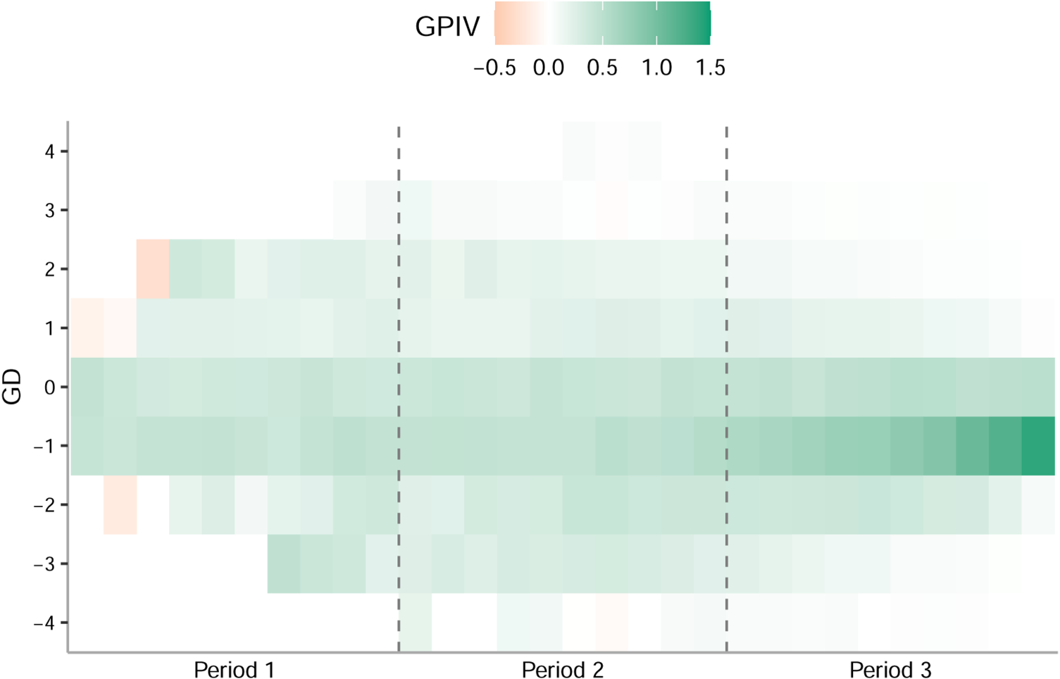
In Figures 2 and 3 we show representative visualizations of the characteristics of GPIV in regulation time. From Figure 2 we note that the value of GPIV is high when the GD is $- 1$ or 0 at the end of the third period, as scoring then will tie the game (going from 0 to 1 PTS) or result in a 1 goal lead (going from 1 to 2 PTS). However, as the scoring frequency in the last minute is three times higher than at any other arbitrary minute in the game (see Figure 1), this increase in GPIV may not be as high as expected.

Figure 2.

GPIV versus GD for the 2013-2014 season. Each bin is two minutes. Bins with less than two observations are left out.

Figure 3.

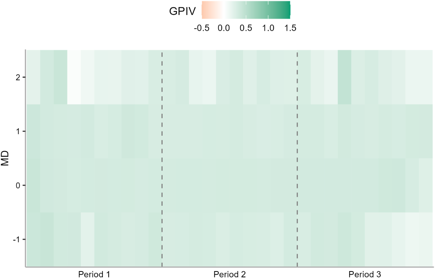
GPIV versus MD for the 2013-2014 season. Each bin is two minutes. Bins with less than two observations are left out.

Scoring goals is not always positive for the probability of earning PTS. We observed that, although this situation rarely appears, taking a 3-goal lead early in the game may have negative consequences. This could be explained by the possibility of the leading team becoming too complacent with a comfortable lead. In general, negative consequences were limited to the first period.

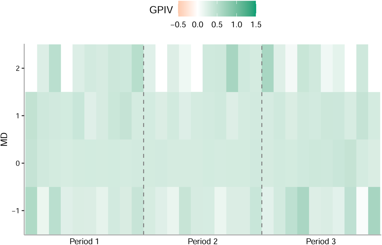
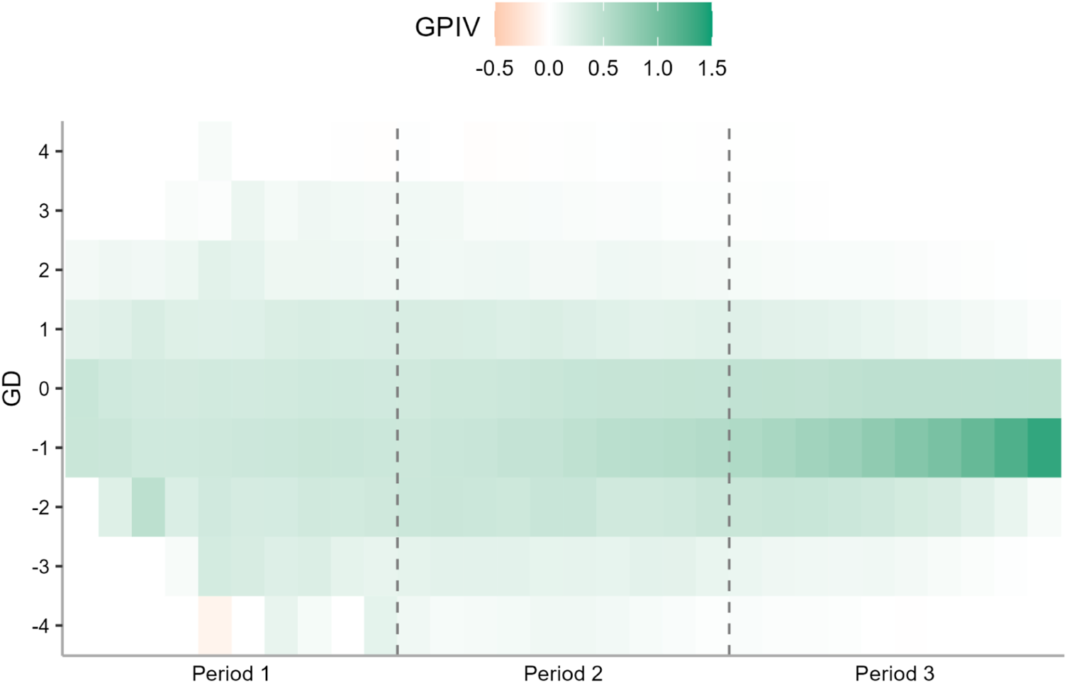
Figures 4 and 5 shows the characteristics of GPIV in regulation time with respect to GD when computed over the data for all seasons in the data set. We note that the change of values for GPIV from a bin to a neighboring bin is slightly smoother than when the values are computed for one season and thus may be more intuitive.⁷ However, as there does not seem to be a large difference between the results for different seasons, in our work, we have chosen to compute values based on one season. The advantage is that the data set used for computation is smaller and that only recent historical data is needed.

Figure 4.

GPIV versus GD computed over all seasons in the data set. Each bin is two minutes. Bins with less than two observations are left out.

Figure 5.

GPIV versus MD computed over all seasons in the data set. Each bin is two minutes. Bins with less than two observations are left out.

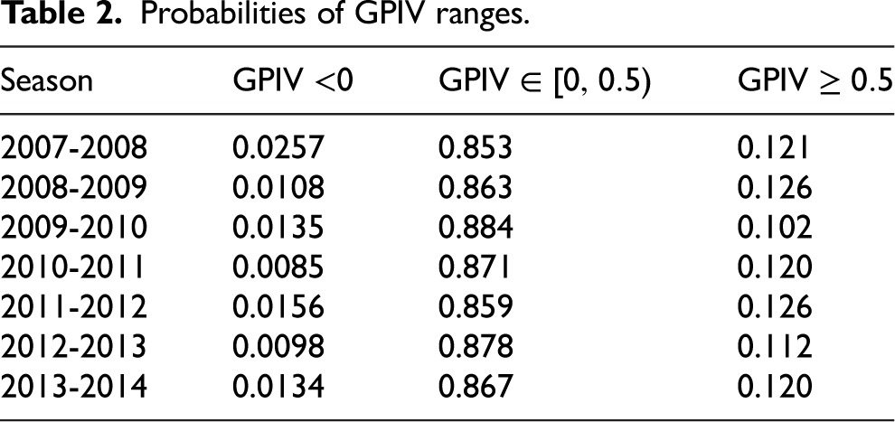
In Table 2 we show the probabilities for negative GPIV, GPIV between 0 and 0.5, as well as GPIV higher than 0.5. What is interesting about this last group, is that they have the same or greater GPIV as overtime goals (0.5). As an example, for the 2013-2014 season, the probability of a negative GPIV is 1.3%. Approximately 86.7% of the GPIV range from 0 to 0.5. Furthermore, 12.0% of the GPIV range from 0.5 to 1.5. In general, the probabilities are relatively stable over different seasons.

Table 2.

Probabilities of GPIV ranges.

Season	GPIV $< 0$	GPIV $\in [0, 0.5)$	GPIV $\geq 0.5$
2007-2008	0.0257	0.853	0.121
2008-2009	0.0108	0.863	0.126
2009-2010	0.0135	0.884	0.102
2010-2011	0.0085	0.871	0.120
2011-2012	0.0156	0.859	0.126
2012-2013	0.0098	0.878	0.112
2013-2014	0.0134	0.867	0.120

New metrics

We define new variants of the traditional metrics goals (G), assists (A), points (P), and $+ / -$ which we call GPIV-G, GPIV-A, GPIV-P, and GPIV- $+ / -$ , respectively. In the traditional metrics the value is raised by 1 when a player scores a goal (for G and P), a player gives an assist to a goal (for A and P) or the player is on the ice when a goal is scored by the player’s team (for $+ / -$ ). For the latter, when a goal is scored by the opposing team, the value is decreased by 1. For the variants of the metrics, instead of raising or decreasing by 1, we raise or decrease the value by the GPIV of the goal. The new metrics value the amount of goals as well as the importance of these goals. Some of the highest-ranked players are involved in many goals, while others may be involved in fewer goals, but with higher importance.

Further, it may be interesting to look at the average importance of the goals in which a player is involved as scorer, assist giver or both. This importance can be obtained by dividing the new metrics by the old metrics. For instance, GPIV-P/P is a measure of the average importance of the goals in which a player is involved with respect to points (as scorer or as assist giver). Similarly, GPIV-A/A is the average importance of the goals in which a player is involved as assist giver, and GPIV-G/G is the average importance of the goals a player scores. We note that for a traditional metric X, as GPIV-X = (GPIV-X/X) * X, it means that GPIV-X is the traditional metric X for a player weighted by the average importance of the goals contributing to X in which that player was involved.

We note that team situation is an issue for most metrics. Better teams score more goals. Therefore, it is easier for players in the better teams to obtain higher values for traditional metrics such as G, A, and P, as well as for the new counterparts GPIV-G, GPIV-A and GPIV-P. However, the new metrics reduce the influence of this issue somewhat. First, although good teams score more, the importance of the goals is reduced when the team is leading. Therefore, for the GPIV-based metrics the addition of not so important goals does not raise the relative value of the metric as much as for the traditional metrics. Secondly, GPIV-X/X shows the average importance of the goals contributing to X, and thus even in worse teams, a player can have a high value for this metric (by e.g., often being involved in tying and lead-taking goals).

In the following sections, we look at the characteristics of the new metrics and show how players and player pairs performed according to these metrics.

Eye test for GPIV metrics

In this section, we check whether the metrics pass the eye test. We discuss the 2013-2014 season as a representative season with a focus on GPIV-P, GPIV-A, GPIV-P, the team they played (most) for and the final team rank after the season.

The tables in this section contain the following information: rank according to the traditional metric, rank according to the new metric, rank change (old rank minus new rank), player name, player position, old metric value, new metric value, and new metric value divided by the old metric value (representing the average importance of goals that the player is involved in for this metric). Further, there is information about which team the players played for as well as the team rank at the end of the season.

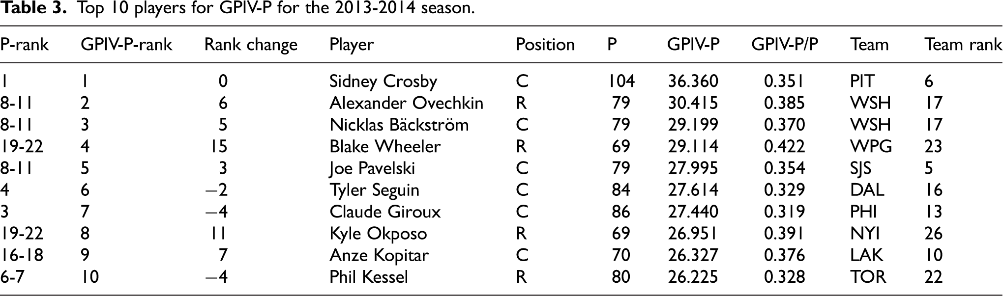
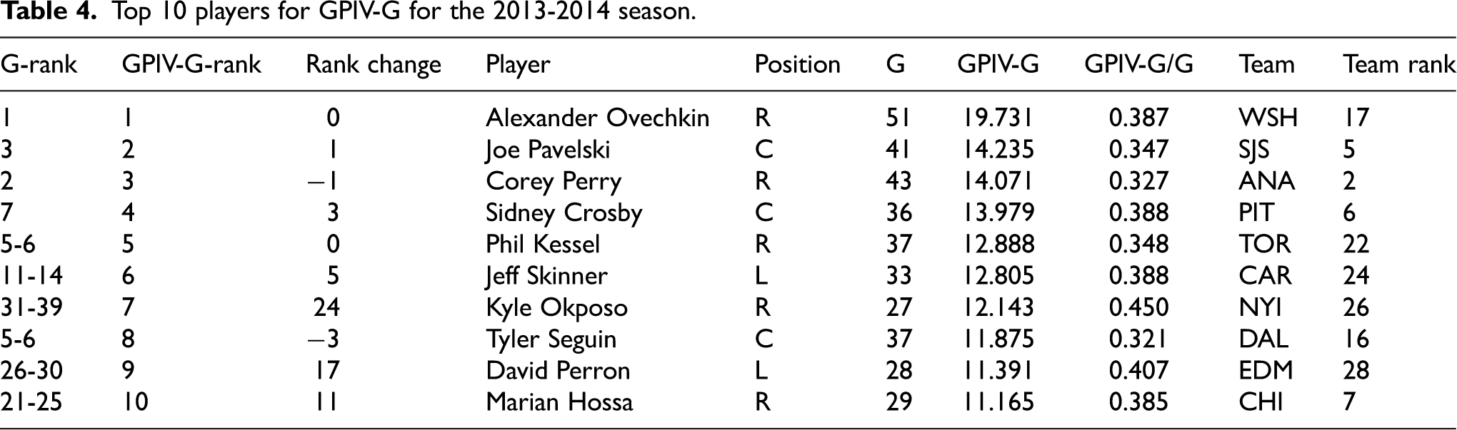
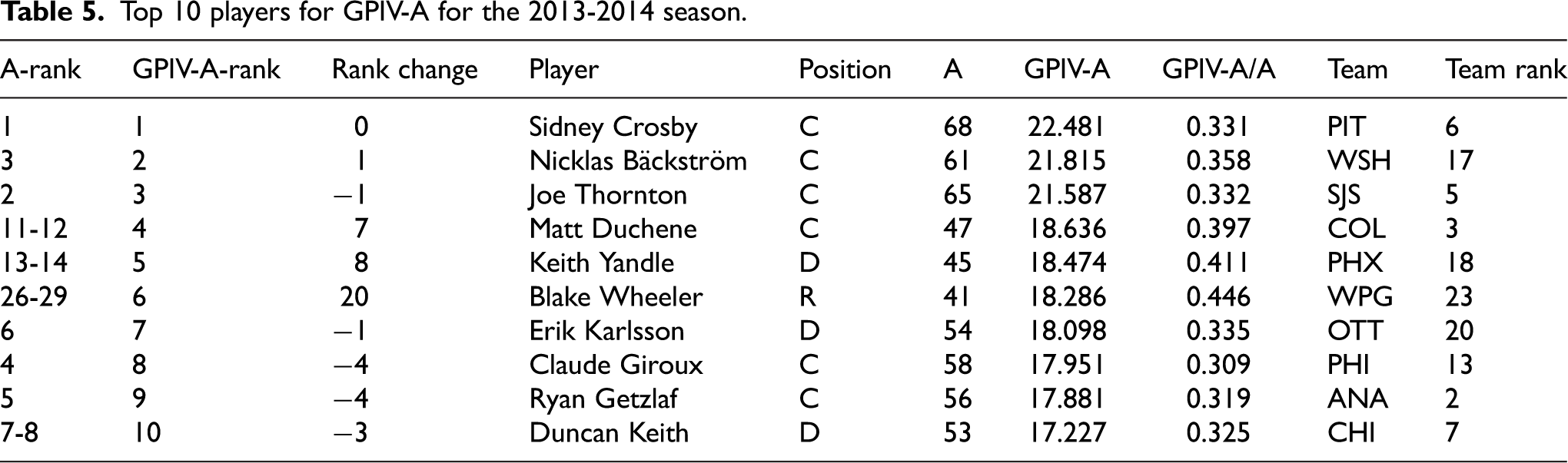
Tables 3, 4, and 5 show the top-ranked players for GPIV-P, GPIV-G, and GPIV-A during the 2013-2014 season, respectively. Regarding GPIV-P several players stand out. First, Alexander Ovechkin had a rank of 8-11 for P but had a rank of 2 for GPIV-P. This is a considerable difference in rank but can be explained by the many important goals he scored that season. For example, as mentioned already in the introduction, Alexander Ovechkin had the most game-tying and lead-taking goals while he only ranked 29 $^{th}$ regarding goals scored when the team is already in the lead. Other players on the top-10 list that saw significant increases in their relative point-based rankings were Blake Wheeler (Winnipeg Jets) and Anze Kopitar (LA Kings). Similar to Alexander Ovechkin, the latter of these has proven to take the game to the next level during the playoffs (when goals are tougher to get by and each goal is typically considered of greater value). Similar rank changes are observed for G and A, where players such as Kyle Okposo (for G) and Blake Wheeler (for A) see a noticeably increased ranking, where Kyle Okposo went from rank 31-39 (G) to 7 (GPIV-G) and Blake Wheeler rose to rank 6 (GPIV-A) from rank 26-29 (A).

Table 3.

Top 10 players for GPIV-P for the 2013-2014 season.

P-rank	GPIV-P-rank	Rank change	Player	Position	P	GPIV-P	GPIV-P/P	Team	Team rank
1	1	0	Sidney Crosby	C	104	36.360	0.351	PIT	6
8-11	2	6	Alexander Ovechkin	R	79	30.415	0.385	WSH	17
8-11	3	5	Nicklas Bäckström	C	79	29.199	0.370	WSH	17
19-22	4	15	Blake Wheeler	R	69	29.114	0.422	WPG	23
8-11	5	3	Joe Pavelski	C	79	27.995	0.354	SJS	5
4	6	$- 2$	Tyler Seguin	C	84	27.614	0.329	DAL	16
3	7	$- 4$	Claude Giroux	C	86	27.440	0.319	PHI	13
19-22	8	11	Kyle Okposo	R	69	26.951	0.391	NYI	26
16-18	9	7	Anze Kopitar	C	70	26.327	0.376	LAK	10
6-7	10	$- 4$	Phil Kessel	R	80	26.225	0.328	TOR	22

Table 4.

Top 10 players for GPIV-G for the 2013-2014 season.

G-rank	GPIV-G-rank	Rank change	Player	Position	G	GPIV-G	GPIV-G/G	Team	Team rank
1	1	0	Alexander Ovechkin	R	51	19.731	0.387	WSH	17
3	2	1	Joe Pavelski	C	41	14.235	0.347	SJS	5
2	3	$- 1$	Corey Perry	R	43	14.071	0.327	ANA	2
7	4	3	Sidney Crosby	C	36	13.979	0.388	PIT	6
5-6	5	0	Phil Kessel	R	37	12.888	0.348	TOR	22
11-14	6	5	Jeff Skinner	L	33	12.805	0.388	CAR	24
31-39	7	24	Kyle Okposo	R	27	12.143	0.450	NYI	26
5-6	8	$- 3$	Tyler Seguin	C	37	11.875	0.321	DAL	16
26-30	9	17	David Perron	L	28	11.391	0.407	EDM	28
21-25	10	11	Marian Hossa	R	29	11.165	0.385	CHI	7

Table 5.

Top 10 players for GPIV-A for the 2013-2014 season.

A-rank	GPIV-A-rank	Rank change	Player	Position	A	GPIV-A	GPIV-A/A	Team	Team rank
1	1	0	Sidney Crosby	C	68	22.481	0.331	PIT	6
3	2	1	Nicklas Bäckström	C	61	21.815	0.358	WSH	17
2	3	$- 1$	Joe Thornton	C	65	21.587	0.332	SJS	5
11-12	4	7	Matt Duchene	C	47	18.636	0.397	COL	3
13-14	5	8	Keith Yandle	D	45	18.474	0.411	PHX	18
26-29	6	20	Blake Wheeler	R	41	18.286	0.446	WPG	23
6	7	$- 1$	Erik Karlsson	D	54	18.098	0.335	OTT	20
4	8	$- 4$	Claude Giroux	C	58	17.951	0.309	PHI	13
5	9	$- 4$	Ryan Getzlaf	C	56	17.881	0.319	ANA	2
7-8	10	$- 3$	Duncan Keith	D	53	17.227	0.325	CHI	7

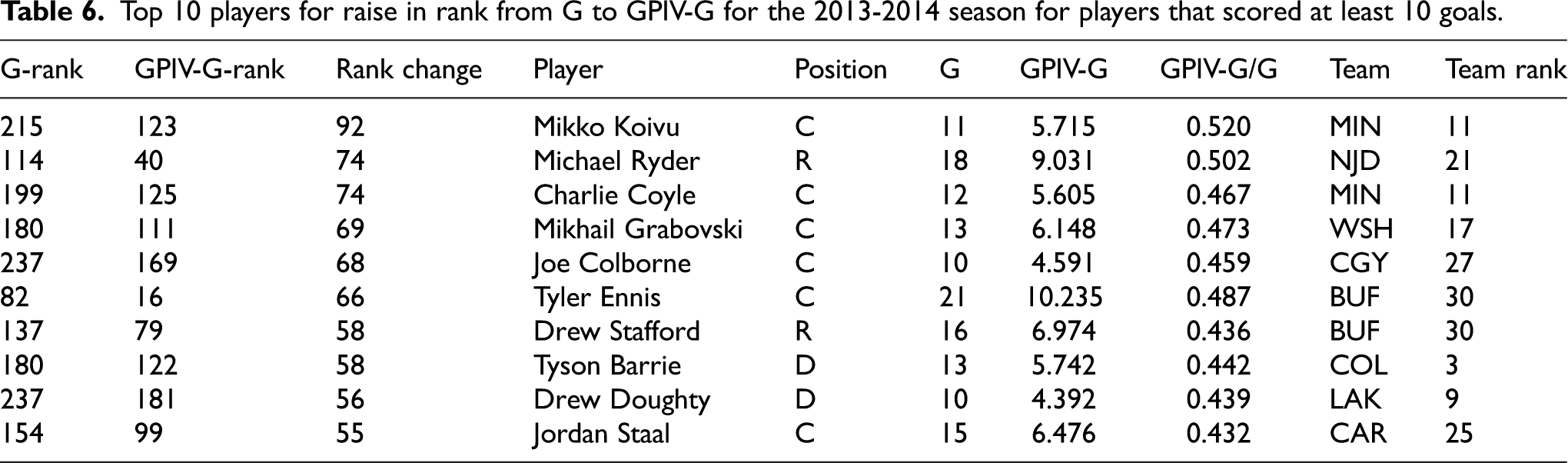
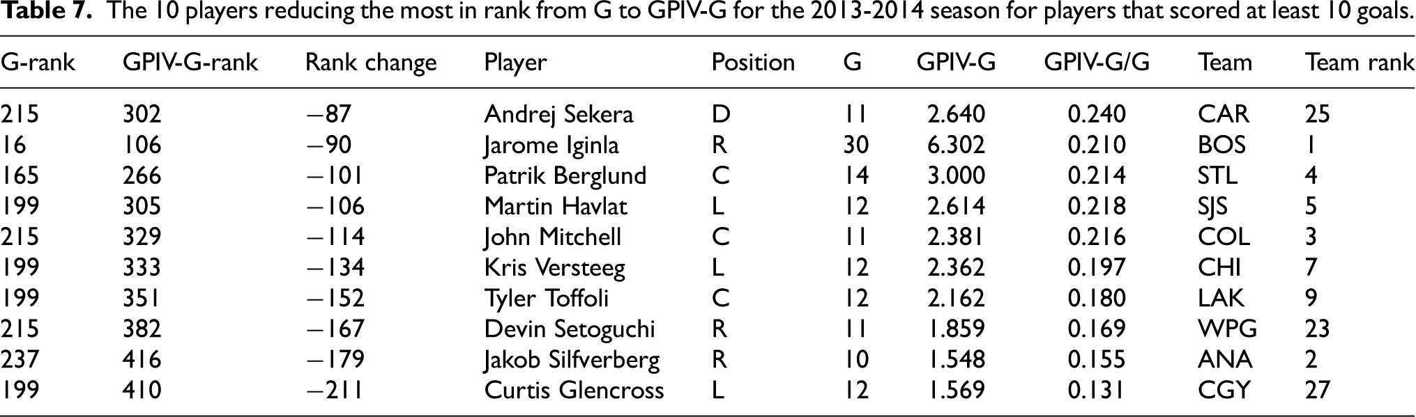
Tables 6 and 7 show the highest absolute changes in rank for goals (GPIV-G vs G) in positive and negative direction, respectively, where we filtered out the players that scored less than ten goals during the season. We note that, in general, in the lower ranges of goals scored, more players have the same rank for G and smaller differences in the number of goals can have a large effect in rank. Therefore, larger jumps in the rank changes can be expected. Further, players with high positive changes in rank have, as expected, a high average importance of the goals in which they are involved (which is reflected in the overlap of Tables 6 and 8), while large negative changes indicate a low average importance of the goals in which they are involved.

Table 6.

Top 10 players for raise in rank from G to GPIV-G for the 2013-2014 season for players that scored at least 10 goals.

G-rank	GPIV-G-rank	Rank change	Player	Position	G	GPIV-G	GPIV-G/G	Team	Team rank
215	123	92	Mikko Koivu	C	11	5.715	0.520	MIN	11
114	40	74	Michael Ryder	R	18	9.031	0.502	NJD	21
199	125	74	Charlie Coyle	C	12	5.605	0.467	MIN	11
180	111	69	Mikhail Grabovski	C	13	6.148	0.473	WSH	17
237	169	68	Joe Colborne	C	10	4.591	0.459	CGY	27
82	16	66	Tyler Ennis	C	21	10.235	0.487	BUF	30
137	79	58	Drew Stafford	R	16	6.974	0.436	BUF	30
180	122	58	Tyson Barrie	D	13	5.742	0.442	COL	3
237	181	56	Drew Doughty	D	10	4.392	0.439	LAK	9
154	99	55	Jordan Staal	C	15	6.476	0.432	CAR	25

Table 7.

The 10 players reducing the most in rank from G to GPIV-G for the 2013-2014 season for players that scored at least 10 goals.

G-rank	GPIV-G-rank	Rank change	Player	Position	G	GPIV-G	GPIV-G/G	Team	Team rank
215	302	$- 87$	Andrej Sekera	D	11	2.640	0.240	CAR	25
16	106	$- 90$	Jarome Iginla	R	30	6.302	0.210	BOS	1
165	266	$- 101$	Patrik Berglund	C	14	3.000	0.214	STL	4
199	305	$- 106$	Martin Havlat	L	12	2.614	0.218	SJS	5
215	329	$- 114$	John Mitchell	C	11	2.381	0.216	COL	3
199	333	$- 134$	Kris Versteeg	L	12	2.362	0.197	CHI	7
199	351	$- 152$	Tyler Toffoli	C	12	2.162	0.180	LAK	9
215	382	$- 167$	Devin Setoguchi	R	11	1.859	0.169	WPG	23
237	416	$- 179$	Jakob Silfverberg	R	10	1.548	0.155	ANA	2
199	410	$- 211$	Curtis Glencross	L	12	1.569	0.131	CGY	27

Table 8.

Top 10 players for GPIV-G/G for the 2013-2014 season for players that scored at least 10 goals.

G-rank	GPIV-G-rank	Rank change	Player	Position	G	GPIV-G	GPIV-G/G	Team	Team rank
215	123	92	Mikko Koivu	C	11	5.715	0.520	MIN	11
114	40	74	Michael Ryder	R	18	9.031	0.502	NJD	21
82	16	66	Tyler Ennis	C	21	10.235	0.487	BUF	30
180	111	69	Mikhail Grabovski	C	13	6.148	0.473	WSH	17
199	125	74	Charlie Coyle	C	12	5.605	0.467	MIN	11
237	169	68	Joe Colborne	C	10	4.591	0.459	CGY	27
31	7	24	Kyle Okposo	R	27	12.143	0.450	NYI	26
73	24	49	Alexander Semin	R	22	9.826	0.447	CAR	25
180	122	58	Tyson Barrie	D	13	5.742	0.442	COL	3
237	181	56	Drew Doughty	D	10	4.392	0.439	LAK	9

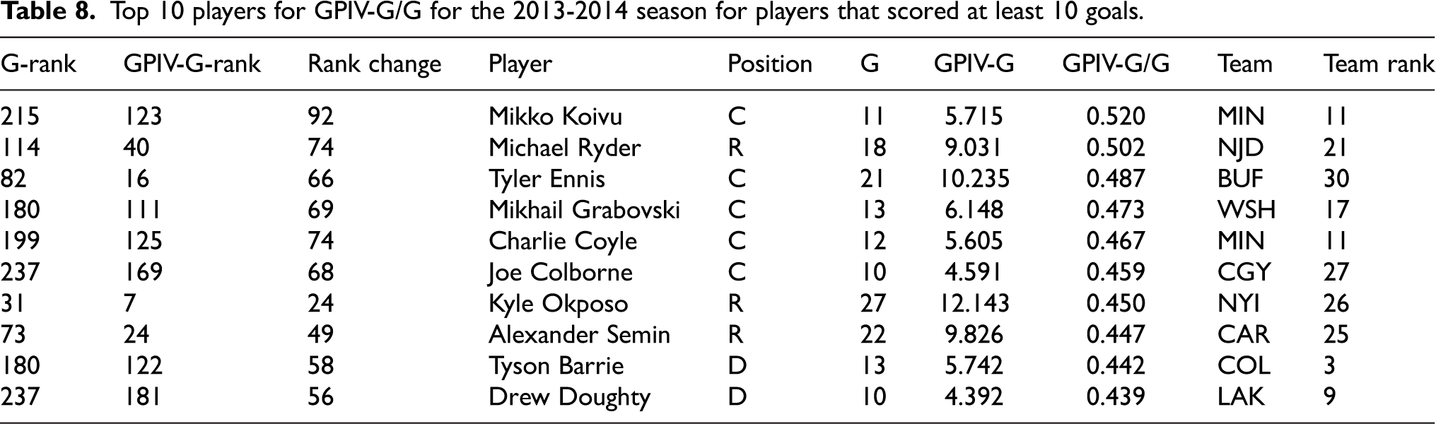
The traditional metrics focus on the number of goals a player is involved in, while the GPIV-based metrics additionally take the importance of the goals into account. Dividing the values of the new metrics with the value of the traditional metrics shows the average importance of the goals in which the players were involved. For points, we see that Blake Wheeler had the highest GPIV-P/P among the top ten GPIV-P players at 0.422 while Claude Giroux had the lowest with 0.319, which aligns with the facts that Wheeler gained ranks and Giroux lost ranks from the traditional to the new metrics. Similarly, Kyle Okposo had the highest GPIV-G/G while gaining 24 ranks from G to GPIV-G, while Blake Wheeler also gained the most ranks from A to GPIV-A with the highest GPIV-A/A among the top ten GPIV-A players.

Table 8 shows the highest average importance values for goal scored (GPIV-G/G) for the players that scored at least ten goals during the 2013-2014 season. The highest average importance for goals as a goal scorer is for Mikko Koivu (0.52) for the 11 goals that he scored during that season. This also explains his raise in rank from 215 to 123 from G to GPIV-G. Of the top ten players regarding GPIV-G, only Kyle Okposo makes it in the top ten for average importance of the goals he scored. The next top 10 player for GPIV-G, David Perron, is on place 24 for the average importance of the goals he scored.

Tables 3 to 7 do not show any obvious correlation between the ranking of players in the different GPIV-based metrics and the ranking of the teams they played for. They contain players for both highly-ranked and lower-ranked teams. Table 8 shows examples for the fact that players in non-top teams can have a high average importance of the goals they are involved. For instance, the top five players in Table 8 played for Minnesota Wild ranked 11 (Mikko Koivu and Charlie Coyle), New Jersey Devils ranked 21 (Michael Ryder), Buffalo Sabres ranked 30 (Tyler Ennis) and Washington Capitals ranked 17 (Mikhail Grabovski). We also do not find any obvious correlation between being involved in empty net goals and the raising or falling in the rankings. As examples, we take the players in Tables 6 (highest raise) and 7 (largest loss) in 2023-2014. The player with the highest rank raise (Mikko Koivu) scored no and conceded 3 empty net goals. The player with the largest rank loss (Andrej Sekera) scored no and conceded 2 empty net goals. Regarding the other players with high rank raise in Table 6, no player scored empty net goals and some conceded empty net goals (Tyson Barrie: 2, Drew Doughty: 4, Jordan Staal: 1). Regarding the other players with high rank loss in Table 7, Jarome Iginla scored 4, Kris Versteeg no, and the other players 1 empty net goal. Jarome Iginla and Patrik Berglund conceded 2, John Mitchell and Kris Versteeg conceded 1, and the other players conceded no empty net goals.⁸

Table 9 shows the top-ranked players for GPIV-G (as in Table 4) and adds information regarding the metrics when the game is close (-1 $\leq$ GD $\leq$ 1), the team of the player is trailing (GD $\leq$ $-$ 2) or winning (GD $\geq$ 2). From the values in the table it can be computed that for these top-ranked players the highest average importance values for goal scored (GPIV-G/G) is highest when the game is close, then when the team is trailing and lowest when the team is winning.

Table 9.

Top 10 players for GPIV-G for the 2013-2014 season.

Player	G	GR	CG	TG	WG	OTG	CGR	TGR	WGR	OTGR
	G*	GR*	CG*	TG*	WG*		CGR*	TGR*	WGR*
Alexander Ovechkin	51	1	37	9	2	3	1	1	130–228	1–3
	19.731	1	15.599	2.473	0.159		1	2	171
Joe Pavelski	41	3	30	2	9	0	2–3	119–213	1–5	115–700
	14.235	2	13.107	0.439	0.689		2	175	6
Corey Perry	43	2	30	4	8	1	2–3	38–63	6–7	13–114
	14.071	3	11.387	1.326	0.858		6	32	1
Sidney Crosby	36	7	29	0	6	1	4–5	420–700	14–22	13–114
	13.979	4	13.100	0	0.379		3	395–691	49
Phil Kessel	37	5–6	29	3	5	0	4–5	64–118	23–42	115–700
	12.888	5	11.500	0.930	0.459		5	65	31
Jeff Skinner	33	11–14	26	3	3	1	9	64–118	76–129	13–114
	12.805	6	11.730	0.130	0.445		4	361	36
Kyle Okposo	27	31–39	19	6	1	1	36–45	9–23	229–386	13–114
	12.143	7	9.736	1.658	0.250		9	14	97
Tyler Seguin	37	5–6	27	3	7	0	7–8	64–118	8–13	115–700
	11.875	8	10.443	0.748	0.684		7	92	7
David Perron	28	26–30	19	7	2	0	36–45	6–8	130–228	115–700
	11.391	9	8.932	2.149	0.310		19	6	69
Marian Hossa	29	21–25	24	2	3	0	10–14	119–213	76–129	115–700
	11.165	10	10.124	0.791	0.249		8	84	98

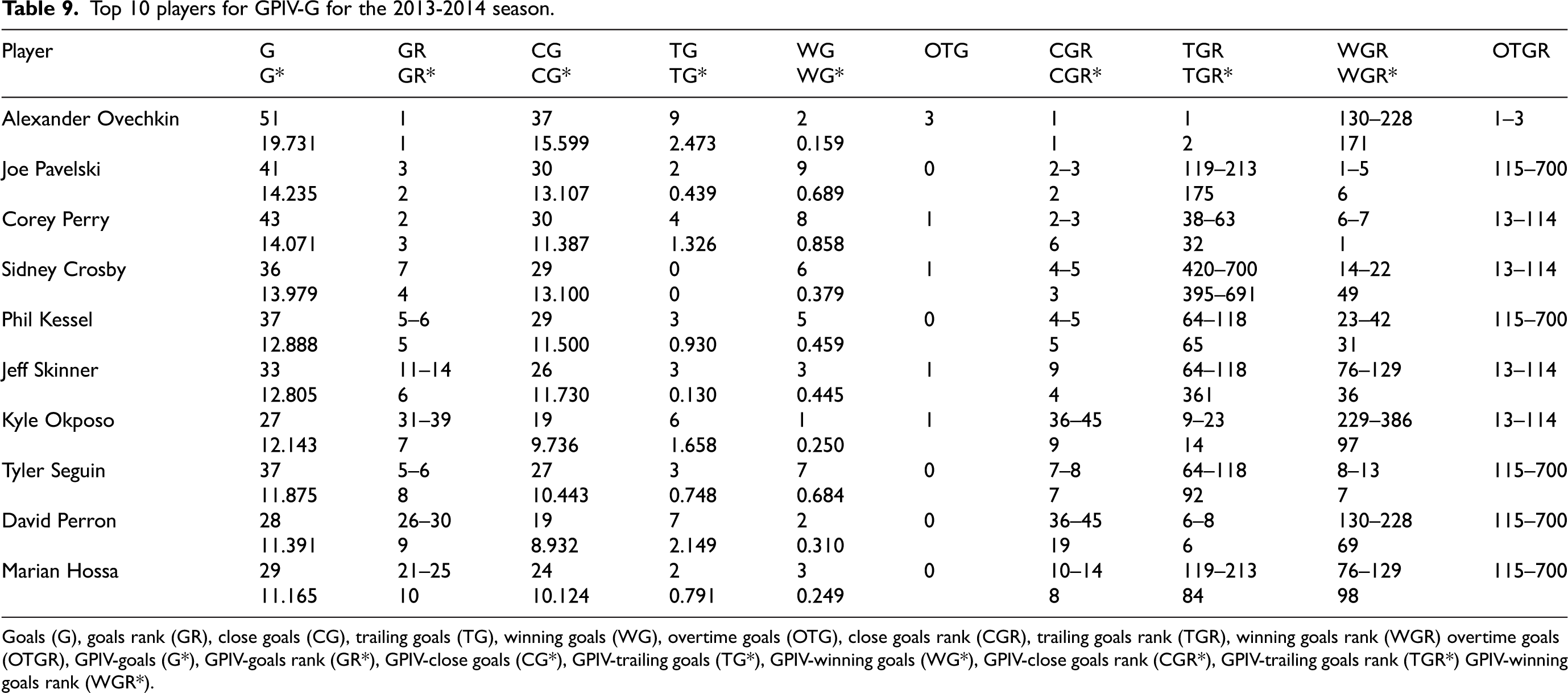
Goals (G), goals rank (GR), close goals (CG), trailing goals (TG), winning goals (WG), overtime goals (OTG), close goals rank (CGR), trailing goals rank (TGR), winning goals rank (WGR) overtime goals (OTGR), GPIV-goals (G*), GPIV-goals rank (GR*), GPIV-close goals (CG*), GPIV-trailing goals (TG*), GPIV-winning goals (WG*), GPIV-close goals rank (CGR*), GPIV-trailing goals rank (TGR*) GPIV-winning goals rank (WGR*).

Correlations of GPIV metrics with traditional metrics

In this section, we investigate the correlations between the GPIV-based metrics and their traditional counterparts. As noted before, GPIV-based metrics are a weighted variant of the traditional counterpart where the weight represents the average importance of the goals in which a player was involved and that contribute to the traditional metric. Therefore, we expect high correlations.

In Table 10 we show the Pearson correlation, the Spearman correlation, and the maximal information coefficient (MIC) between the traditional metrics and their respective new GPIV-based metrics.

Table 10.

Correlation between traditional and GPIV metrics during regular season.

Season	Pearson correlation				Spearman correlation				MIC
Season	Goals	Assists	Points	$+ / -$	Goals	Assists	Points	$+ / -$	Goals	Assists	Points	$+ / -$
2007-2008	0.968	0.979	0.985	0.832	0.964	0.980	0.987	0.789	0.862	0.942	0.940	0.551
2008-2009	0.975	0.979	0.988	0.780	0.970	0.981	0.988	0.744	0.905	0.909	0.944	0.438
2009-2010	0.967	0.975	0.984	0.783	0.963	0.977	0.986	0.719	0.919	0.917	0.945	0.414
2010-2011	0.967	0.974	0.985	0.784	0.968	0.979	0.988	0.759	0.903	0.933	0.967	0.473
2011-2012	0.975	0.977	0.986	0.800	0.969	0.980	0.988	0.776	0.904	0.939	0.953	0.502
2012-2013	0.946	0.966	0.978	0.854	0.947	0.964	0.979	0.827	0.863	0.891	0.954	0.550
2013-2014	0.965	0.973	0.982	0.796	0.971	0.979	0.988	0.775	0.904	0.928	0.946	0.502

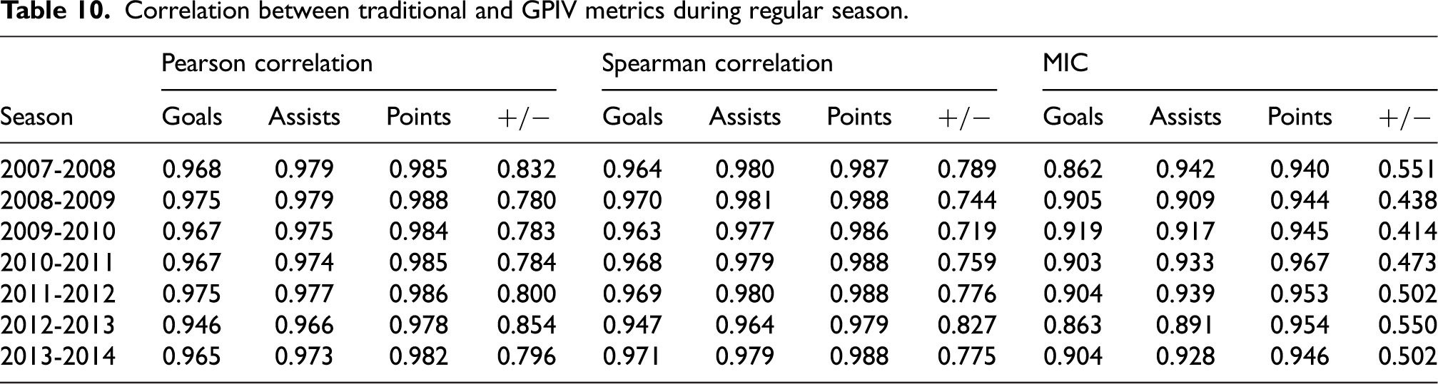
For the Spearman correlation, for goals the correlation is between 0.947 and 0.971, for assists between 0.964 and 0.981, and for points between 0.979 and 0.988. These are high correlations, indicating that the new metrics have similar behavior as well-accepted traditional metrics, but they do introduce new insights.

For $+ / -$ the correlation is lower being between 0.719 and 0.827. This is expected as well. First, the $+ / -$ statistics in general see bigger variations (e.g., from season to season for individual players). Second, $+ / -$ has both an offense component and a defense component, while G, A, P only have an offense component. For GPIV- $+ / -$ both the importance of goals scored and the importance of goals conceded has an influence, while for the GPIV-based variants of G, A, P only the importance of goals scored has an influence. This likely further increases the variation. Third, there may not be a correlation between the importance of goals scored when a player is on the ice and the importance of goals conceded when a player is on the ice. We therefore expect the correlation between $+ / -$ and GPIV- $+ / -$ to be lower than between G, A, P and their counterparts.

In appendix A we show rank comparisons for the top-30 players in the GPIV-based rankings, and we visualize the Spearman correlation as a representative as the observations are similar for the different correlation measures.

Prediction of GPIV metrics

As described in appendices B and C, for the seasons used in our experiments, it seems that using data from earlier seasons leads to a good approximation of the GPIV-based metrics for the current season. In this section, we investigate whether data from part of a season can be used to predict the value of the metric at the end of that season. We do this by dividing the data into partitions. For $n$ partitions, we use the value of the metric after $\frac{1}{n}$ -th part of the season, multiply with $n$ , and compare with the actual result of the metric at the end of the season. We do this for the traditional metrics as well as for the new metrics.

Figure 6 shows for different seasons and different numbers of partitions, the Spearman correlation between final-season metrics and values obtained by using only the smaller partitions to predict the end-of-season value of the same metric for all players.

Figure 6.

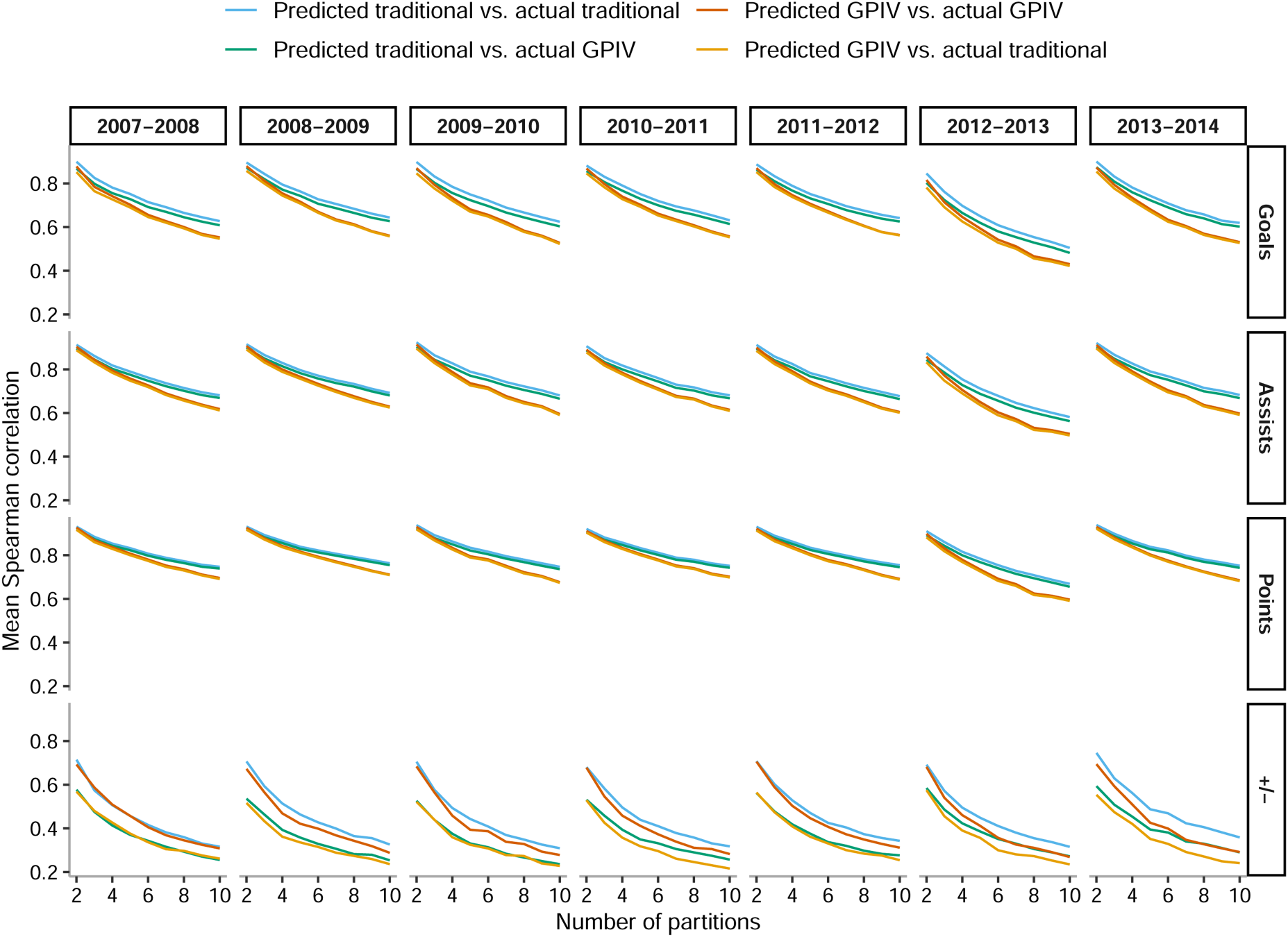
Correlations for partitions for different metrics.

We note that for all metrics, the more partitions, the lower the correlation. This is as expected. For instance, after half of the season ( $n = 2$ ) we have more data to base our prediction on than after one-tenth of a season ( $n = 10$ ). We note that the number of games for one-tenth of the season is about the number of games in the playoffs for which we noted that more rare goal contexts occur (appendix D).

Further, for traditional metrics (in blue) as well as the new metrics (in red) there is a high correlation between the final value and 2 times the value after half of the season. When we have less data, i.e., the number of partitions becomes higher, there is a slightly higher correlation for the traditional metrics than for the new metrics. This can be seen as the gap between the two lines increases with an increasing partition count. In general, the two lines for a given metric also follow a similar trend.

The other colors (green and orange) show predictability between traditional metrics and new metrics, which relates back to the correlation between the metrics. Here, the correlations for the predicted traditional metrics show a higher correlation than for the predicted GPIV-based metrics, with the exception of $+ / -$ . Moreover, the predicted traditional metrics are closely associated with both the traditional and GPIV-based metrics at the end of the season, while the predicted GPIV-based metrics have a somewhat weaker correlation with the end-of-the-season values.

Player pairs

As an input to building successful teams, it is not only interesting to evaluate the performance of individual players, but it is also important to investigate how well players play together. In this paper, we investigate pairs of players. We have chosen to use pairs as in 5-5 play for each team (i) there are two defenders on the ice and (ii) although there are usually three forwards, there is more data available for pairs as the forward lines do change regularly due to, e.g., team strategy or injuries. Using the GPIV-based metrics, we can identify player pairs that share the ice during important goals. We exemplify the method and show results for the 2013-2014 season.

First, we analyze the most prominent player pairs that are directly involved with goals, by either scoring or assisting the goal. The pairs are referred to as a direct pair (DP). In Table 11 we show the sum of the GPIV for all goals for which one player in the pair scored the goal and the other assisted (GPIV-G-DP) together with the number of such goals (G-DP). Further, we divide these goals into goals for which the first player in the pair was the goal scorer (GPIV-G-DP-1 and G-DP-1) and goals for which the second player in the pair was the goal scorer (GPIV-G-DP-2 and G-DP-2).

Table 11.

Top 10 direct pairs for the 2013-2014 season. Player position in parentheses (L for left wing, R for right wing, C for center).

Rank	Player pair	Team	GPIV-G-DP	GPIV-G-DP-1	GPIV-G-DP-2
Rank	Player pair	Team	(G-DP)	(G-DP-1)	(G-DP-2)
1	Jamie Benn (L), Tyler Seguin (C)	DAL	13.96 (45)	7.42 (23)	6.54 (22)
2	Chris Kunitz (L), Sidney Crosby (C)	PIT	12.92 (39)	6.63 (26)	6.29 (13)
3	Corey Perry (R), Ryan Getzlaf (C)	ANA	12.30 (39)	8.66 (25)	3.64 (14)
4	Alex Ovechkin (R), Nicklas Backstrom (C)	WSH	12.27 (35)	10.61 (29)	1.66 (6)
5	Phil Kessel (R), James van Riemsdyk (L)	TOR	11.56 (34)	5.88 (17)	5.68 (17)
6	Andrew Ladd (L), Bryan Little (C)	WPG	11.05 (29)	5.98 (15)	5.07 (14)
7	Paul Stastny (C), Gabriel Landeskog (L)	COL	9.65 (24)	5.15 (14)	4.50 (10)
8	Claude Giroux (C), Jakub Voracek (R)	PHI	9.50 (29)	5.74 (14)	3.75 (15)
9	Kyle Okposo (R), John Tavares (C)	NYI	8.98 (24)	5.95 (14)	3.03 (10)
10	David Krejci (C), Milan Lucic (L)	BOS	8.78 (27)	4.47 (10)	4.31 (17)

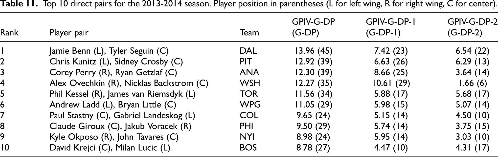
The DPs ranked top ten according to GPIV-G-DP are shown in Table 11. Among these ten pairs, the pair tends to consist of a center and a wing, with the exception of the wing pair Phil Kessel and James van Riemsdyk. Another noteworthy observation is that the most productive pair with respect to GPIV-G-DP-1 or GPIV-G-DP-2 is Alexander Ovechkin and Nicklas Bäckström with Ovechkin the goal scorer and Bäckström providing the assists (in the table GPIV-G-DP-1). For this pair the distribution of these roles is quite clear as the impact according to GPIV-G-DP-2 for this pair is low.

As the direct involvement with a goal does not reflect who was on the ice during the important goals, we also investigate the pairs of players that were on the ice when a goal was scored. These pairs are denoted as indirect pairs (IP) in Table 12. We look at the number of goals scored by the team (GF-IP), conceded by the team (GA-IP), and the goal difference for the team (GD-IP) when both players of the team are on the ice. We also introduce the GPIV variants of these metrics, i.e., GPIV-GF-IP, GPIV-GA-IP, and GPIV-GD-IP, respectively.

Table 12.

Top 10 indirect pairs for the 2013-2014 season. Player position in parentheses (L for left wing, R for right wing, C for center).

Rank	Player pair	Team	GPIV-GD-IP	GPIV-GF-IP	GPIV-GA-IP
Rank	Player pair	Team	(GD-IP)	(GF-IP)	(GA-IP)
1	Sidney Crosby (C), Chris Kunitz (L)	PIT	27.39 (79)	40.60 (117)	13.21 (38)
2	Claude Giroux (C), Jakub Voracek (R)	PHI	22.68 (52)	35.74 (98)	13.05 (46)
3	Joe Pavelski (C), Joe Thornton (C)	SJS	20.64 (57)	27.95 (77)	7.31 (20)
4	Wayne Simmonds (R), Scott Hartnell (L)	PHI	20.16 (42)	23.54 (60)	3.39 (18)
5	Tyler Seguin (C), Jamie Benn (L)	DAL	19.87 (56)	32.23 (101)	12.36 (45)
6	Wayne Simmonds (R), Claude Giroux (C)	PHI	19.03 (33)	21.22 (53)	2.19 (20)
7	Wayne Simmonds (R), Jakub Voracek (R)	PHI	18.51 (33)	19.45 (46)	0.94 (13)
8	Sidney Crosby (C), Matt Niskanen (D)	PIT	18.39 (49)	22.09 (63)	3.70 (14)
9	Ryan Getzlaf (C), Corey Perry (R)	ANA	18.21 (58)	31.66 (102)	13.46 (44)
10	Jakub Voracek (R), Kimmo Timonen (D)	PHI	18.11 (41)	23.07 (56)	4.96 (15)

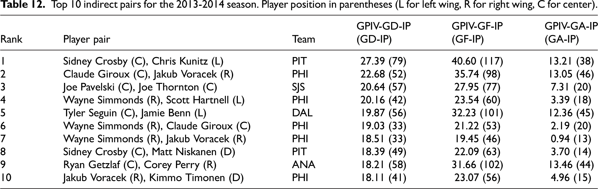
In Table 12 we show the top ten pairs according to GPIV-GD-IP. Among these ten, three pairs also rank within the top ten for direct involvement: Sidney Crosby and Chris Kunitz, Jamie Benn and Tyler Seguin, as well as Claude Giroux and Jakub Voracek, which indicates their importance for offensive production in crucial moments. When considering the teams the players represent, the Philadelphia Flyers stand out with five out of ten pairs (ranks 2, 4, 6, 7, and 10).⁹ Another detail that can also be discerned is that some player pairs conceded few important goals when playing together, e.g., Sidney Crosby and Matt Niskanen, as well as Wayne Simmonds and Jakub Voracek. There may be different reasons for this, ranging from high defensive skills to players mainly being used in offense and often starting in the offensive zone. We note that similarly to the case of single players, the rankings for the GPIV-based metrics for player pairs may be different from the rankings for the traditional metrics. For instance, the pair with Wayne Simmonds and Jakub Voracek is ranked seventh with respect to GPIV-GD-IP but has a lower GD-IP than the pairs ranked 6 to 10.

Conclusion

In this paper, we have introduced new metrics that are variants of the well-known traditional metrics G, A, P, and $+ / -$ . In addition to the number of goals scored, these new metrics also take into account the importance of goals with respect to earning PTS. This ensures that the metrics favor players that have a greater impact on the outcome of the game (e.g., by scoring game-deciding goals) over players that score most of their goals when the outcome of a game may already be decided. As the metrics are based on well-known metrics, they are easily understandable for practitioners. We investigated both regular seasons and playoffs. The new metrics pass the eye test. For G, A, and P there is a high correlation between the traditional metrics and the GPIV-based counterparts, while still bringing new insights. We showed that for the seasons in the experiments, data from the previous seasons can be used to approximate the values for the new metrics for the current season. We also showed that data from the same season can be used to predict the values for the metrics at the end of the season. Further, we showed how to use the metrics to gain insights into the performance of player pairs.

Footnotes

Acknowledgements

Thanks to Rabnawaz Jansher, Sofie Jörgensen, Min-Chun Shih and Jon Vik for implementations in the early stages that were used to decide on the current versions of the metrics.

Funding

The author(s) received no financial support for the research, authorship, and/or publication of this article.

Declaration of conflicting interests

The authors declared no potential conflicts of interest with respect to the research, authorship, and publication of this article.

Notes

References

Bransen

Van Haaren

(2020) Player chemistry: striving for a perfectly balanced soccer team. In: MIT Sloan sports analytics conference.

Brimberg

Hurley

(2009) A note on the importance of the first goal in a national hockey league game. International Journal of Operational Research 6(2): 282–287.

Brimberg

Hurley

(2012) Do professional hockey teams with a two-goal lead lose more often than they should? International Journal of Operational Research 15(2): 226–233.

Chaikof

Clément-Heydra

Markey

Nahabedian

Pilotte

Shaw

(2022) Scouting automated ratings analyzing habits (SARAH): a statistical methodology for scouting and player development. In: Lambrix P, Carlsson N and Vernblom M (eds) Proceedings of the Linköping Hockey Analytics Conference LINHAC 2022 Research Track, pp. 37–48. Linköping Electronic Conference Proceedings.

Decroos

Bransen

Van Haaren

Davis

(2019) Actions speak louder than goals: valuing player actions in soccer. In: Proceedings of the 25th ACM SIGKDD international conference on knowledge discovery & data mining, pp. 1851–1861.

Farah

Baker

(2020) Rough draft: the accuracy of athlete selection in North American professional sports. In: Talent identification and development in sport. Routledge, pp. 145–157.

Farah

Baker

(2021) Accuracy from the slot: evaluating draft selections in the national hockey league. Scandinavian Journal of Medicine & Science in Sports 31(3): 564–572.

Gill

(2000) Late-game reversals in professional basketball, football, and hockey. The American Statistician 54(2): 94–99.

Gramacy

Jensen

Taddy

(2013) Estimating player contribution in hockey with regularized logistic regression. Journal of Quantitative Analysis in Sports 9(1): 97–111.

10.

Foster

Shang

Wei

(2019) A game-predicting expert system using big data and machine learning. Expert Systems with Applications 130: 293–305.

11.

Johansson

Wilderoth

Sattari

(2022) How analytics is changing ice hockey. In: Patrick Lambrix, Niklas Carlsson, and Mikael Vernblom, editors, Proceedings of the Linköping hockey analytics conference LINHAC 2022 research track, pp. 49–59. Linköping Electronic Conference Proceedings.

12.

Kaplan

Mongeon

Ryan

(2014) A markov model for hockey: manpower differential and win probability added. INFOR Information Systems and Operational Research 52(2): 39–50.

13.

Kumagai

Moreau

Kroetch

(2022) Predicting the nhl draft with rank-orderedlogit models. In: Patrick Lambrix, Niklas Carlsson, and Mikael Vernblom, editors, Proceedings of the Linköping hockey analytics conference LINHAC 2022 research track, pp. 60–70. Linköping Electronic Conference Proceedings.

14.

Lehmus Persson

Kozlica

Carlsson

Lambrix

(2020) Prediction of tiers in the ranking of ice hockey players. In: Brefeld U, Davis J, Van Haaren J, and Zimmermann A (eds) Machine Learning and Data Mining for Sports Analytics. MLSA 2020, volume 1324 of Communications in Computer and Information Science, pp. 89–100.

15.

Liu

Schulte

(2018) Deep reinforcement learning in ice hockey for context-aware player evaluation. In: Lang J (ed) Proceedings of the Twenty-Seventh international joint conference on artificial intelligence, pp. 3442–3448.

16.

Ljung

Carlsson

Lambrix

(2019) Player pairs valuation in ice hockey. In: Brefeld U, Davis J, Van Haaren J, and Zimmermann A (eds) Machine Learning and Data Mining for Sports Analytics. MLSA 2018, volume 11330 of Lecture Notes in Computer Science, pp. 82–92.

17.

Macdonald

(2011) A regression-based adjusted plus-minus statistic for NHL players. Journal of Quantitative Analysis in Sports 7(3).

18.

Nandakumar

Jensen

(2019) Historical perspectives and current directions in hockey analytics. Annual Review of Statistics and Its Application 6(1): 19–36.

19.

Perera

Swartz

(01 2012) Resource estimation in T20 cricket. IMA Journal of Management Mathematics 24(3): 337–347.

20.

Pettigrew

(2015) Assessing the offensive productivity of NHL players using in-game win probabilities. In: MIT Sloan Sports Analytics Conference.

21.

Routley

Schulte

(2015) A Markov Game Model for Valuing Player Actions in Ice Hockey. In: Meila M and Heskes T (eds) Uncertainty in Artificial Intelligence, pp. 782–791.

22.

Säfvenberg

Carlsson

Lambrix

(2023) Simple and practical goal importance metrics for ice hockey. In: Brecht T, Carlsson N, Vernblom M, and Lambrix P (eds) Proceedings of the Linköping Hockey Analytics Conference LINHAC 2023 Research Track, volume 201 of Linköping Electronic Conference Proceedings, pp. 40–52.

23.

Sans Fuentes

Carlsson

Lambrix

(2019) Player impact measures for scoring in ice hockey. In: Karlis D, Ntzoufras I, and Drikos S (eds) MathSport International 2019 Conference, pp. 307–317.

24.

Sarlis

Tjortjis

(2020) Sports analytics: evaluation of basketball players and team performance. Information Systems 93: 101562.

25.

Schuckers

Curro

(2013) Total Hockey Rating (THoR): a comprehensive statistical rating of National Hockey League forwards and defensemen based upon all on-ice events. In: MIT Sloan Sports Analytics Conference.

26.

Schulte

Khademi

Gholami

Zhao

Javan

Desaulniers

(2017a) A markov game model for valuing actions, locations, and team performance in ice hockey. Data Mining and Knowledge Discovery 31(6): 1735–1757.

27.

Schulte

Zhao

Javan

Desaulniers

(2017b) Apples-to-apples: clustering and Ranking NHL Players Using Location Information and Scoring Impact. In: MIT Sloan Sports Analytics Conference.

28.

Singh

(2020) Sport analytics: a review. The International Technology Management Review 9(1): 64–69.

29.

Thomas

Ventura

Jensen

(2013) Competing process hazard function models for player ratings in ice hockey. The Annals of Applied Statistics 7(3): 1497–1524.

30.

Tingling

(2017) Educated Guesswork: drafting in the National Hockey League. In: Handbook of Statistical Methods and Analyses in Sports. Chapman and Hall/CRC, pp. 343–356.

31.

Van Roy

Robberechts

Yang

W-C

De Raedt

Davis

(2021) Leaving goals on the pitch: evaluating decision making in soccer. In: MIT Sloan Sports Analytics Conference.

Goal-based performance metrics for ice hockey accounting for goal importance

Abstract

Keywords

Introduction

Related work - measuring performance in ice hockey

Defining a metric

Data

Intuition behind metric

Metrics definition - GPIV-weighted performance metrics

Game Points Importance Value (GPIV) - regular season

Defining an importance value

GPIV with accounting for rare goals in regulation time

Characteristics of GPIV

New metrics

Eye test for GPIV metrics

Correlations of GPIV metrics with traditional metrics

Prediction of GPIV metrics

Player pairs

Conclusion

Footnotes

Acknowledgements

Funding

Declaration of conflicting interests

Notes

References