
Abstract
Plasma lipoproteins are the primary means of lipid transport among tissues. Defining alterations in lipid metabolism is critical to our understanding of disease processes. However, lipoprotein measurement is limited to specialized centers. Preparation for ultracentrifugation involves the formation of complex density gradients that is both laborious and subject to handling errors. We created a fully automated device capable of forming the required gradient. The design has been made freely available for download by the authors. It is inexpensive relative to commercial density gradient formers, which generally create linear gradients unsuitable for rate-zonal ultracentrifugation. The design can easily be modified to suit user requirements and any potential future improvements. Evaluation of the device showed reliable peristaltic pump accuracy and precision for fluid delivery. We also demonstrate accurate fluid layering with reduced mixing at the gradient layers when compared to usual practice by experienced laboratory personnel. Reduction in layer mixing is of critical importance, as it is crucial for reliable lipoprotein separation. The automated device significantly reduces laboratory staff input and reduces the likelihood of error. Overall, this device creates a simple and effective solution to formation of complex density gradients.
Introduction
Lipoproteins are essential components of human metabolism, serving as the transport mechanism for hydrophobic lipids through intracellular and extracellular water. Their synthesis in the liver and gut allow delivery of ingested or hepatically derived cholesterol and triglyceride to distant sites for utilization or storage. Clinicians and researchers have long been interested in lipoproteins, not only for their importance in normal metabolism, but also for their direct involvement in the pathophysiology of common diseases, including atherosclerosis and diabetes.1,2 In these conditions, the normal balance of cholesterol and triglyceride transport is disrupted, resulting in tissue and organ accumulation with disease-causing consequences. Understanding these pathophysiologic changes of lipoprotein metabolism continues to be critical to our understanding of many disease states.
Lipoprotein classification is based on the practical methods used to separate them from plasma. The gold standard technique for separation of lipoproteins is density gradient ultracentrifugation. 3 Classification is based on the relative densities of the aggregates. However, measurement of lipoproteins by this technique is primarily limited to research or specialized laboratories, as it is laborious and requires specialized equipment. Formation of the complex density gradient required for separation is tedious and subject to handling difficulties that can potentially disturb the gradient layers. Mixing of layers must be avoided, as accurate collection of lipoprotein fractions relies on separation at these points. There have long been attempts to try to aid the process of formation of the gradient. 4 Commercial density gradient formers are available (e.g., Eppendorf epMotion 5070/5075, Hamburg, Germany), but expensive or limited in their function. The majority are designed to develop linear gradients (e.g., Gradient Makers, C.B.S. Scientific, Del Mar, CA, or Gradient Mixer, Sigma-Aldrich, St. Louis, MO), unsuitable for zonal ultracentrifugation. We sought to develop an automated system able to form density gradients suitable for zonal ultracentrifugation that was efficient, accurate, and inexpensive.
Materials and Methods
Principle
In solution, particles with density higher than that of the solvent sink (sediment), and those lighter float. The greater the difference in density, the faster the movement, deemed sedimentation and flotation rates, respectively. If there is no difference in density (isopycnic), particles do not move. To take advantage of even tiny differences in density, centrifugal force is applied to accelerate the separation process. Lipoproteins of varying densities are separated from plasma using this principle. Plasma is adjusted to a density above that of the densest lipoproteins using salt (sodium bromide [NaBr] or potassium bromide [KBr]) and centrifuged to allow flotation and separation at the surface.
In order to avoid the problem of cross-contamination of particles of different sedimentation rates that occurs in differential centrifugation ( Fig. 1 ), rate-zonal centrifugation is used. 5 This involves layering a density gradient over samples, allowing particles to float through plasma and gradient, respectively, at a rate dependent on their density and the centrifugal force applied. The rate of flotation of lipoproteins, Svedberg flotation rate (Sf), using rate-zonal centrifugation has been previously determined: VLDL1 (Sf 60–400), VLDL2 (Sf 20–60), IDL (Sf 12–20), and LDL (Sf 0–12). 6
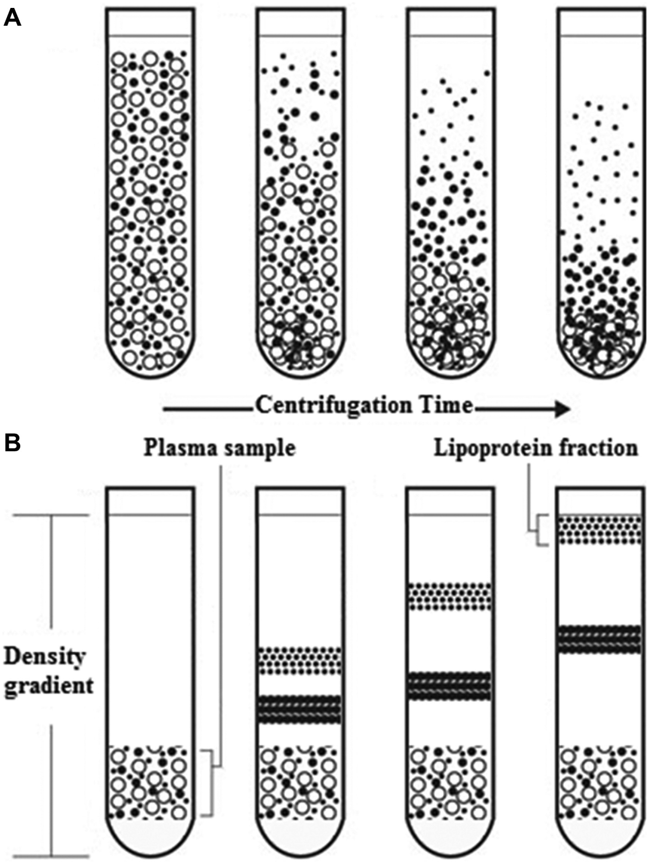
Comparison of (
Density Gradient
To achieve the discontinuous density gradient required for lipoprotein separation from plasma, samples are carefully overlaid with fixed-density salt solutions. Layering is achieved in an ultracentrifuge tube coated with polyvinyl alcohol. 7 This allows solutions to gravity feed down the side of the tubes smoothly, minimizing disruption to formation of the gradient. The lipoprotein separation technique described here is a modification of the method of Lindgren et al. 8 The density of 2 mL of plasma is adjusted to 1.118 g/mL by the addition of 0.341 g sodium chloride and is carefully layered over a cushion of 0.5 mL density 1.182 g/mL sodium bromide solution. The discontinuous gradient is completed by overlayering 1.0988 g/mL (1 mL), 1.0860 g/mL (1 mL), 1.0790 g/mL (2 mL), 1.0722 g/mL (2 mL), 1.0641 g/mL (2 mL), and 1.0588 g/mL (2 mL) sodium bromide solutions.
Automation
To perform this task repeatedly, with precision, minimizing laboratory staff input and avoiding disruption of the gradient, an automated instrument was created ( Fig. 2 ). The complete design of all components, electronic circuitry, and software for the device can be downloaded (https://www.dropbox.com/sh/dbj4lnr03kak4lw/AAAnC3F_KCQW1N3JvQz–e0Ga?oref=e&n=457599943). This instrument is designed to handle six samples per run, as ultracentrifugation is performed using a six-bucket SW40Ti rotor (Beckman Coulter [UK] Ltd., High Wycombe, UK). However, the number of samples could be altered to requirements if necessary.
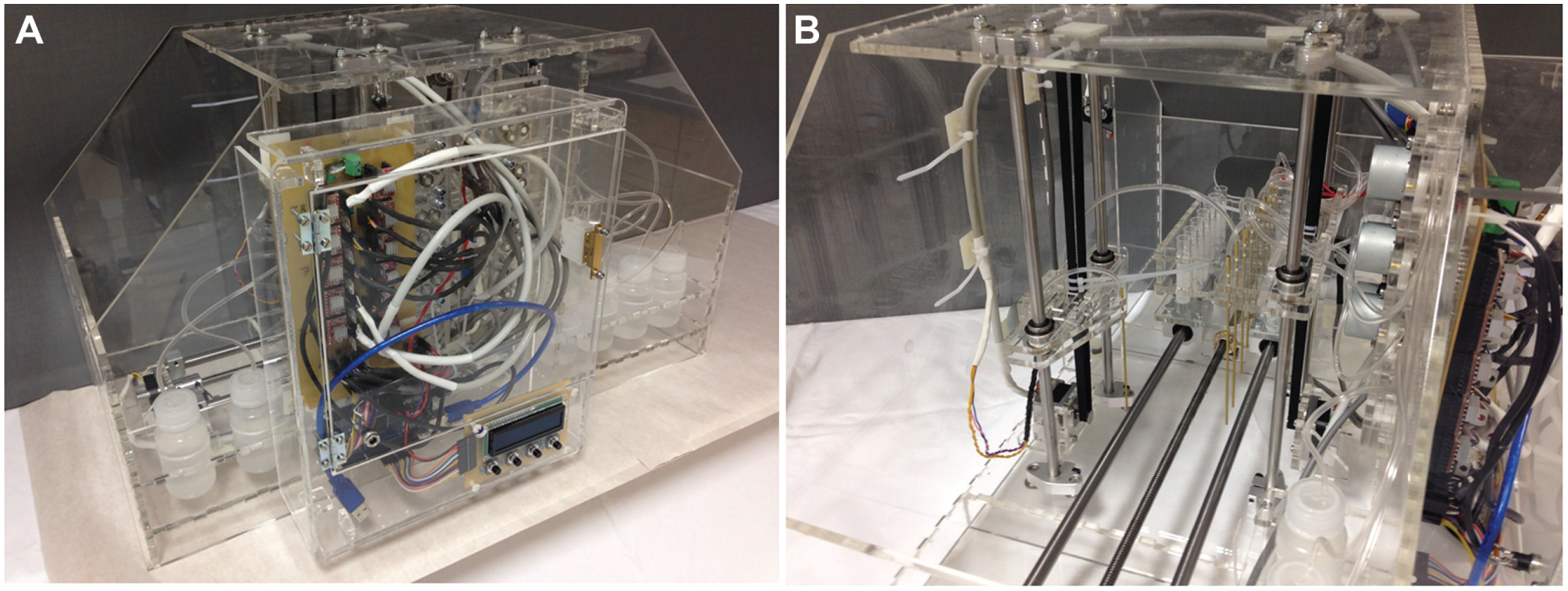
Automated device for the formation of rate-zonal ultracentrifugation density gradients. (
Design
The design principle was to have six ultracentrifuge tubes move through eight filling stations. Stations 1 and 3–8 would progressively layer fixed-density sodium bromide solutions. Station 2 would layer density-adjusted plasma samples over the cushion of fluid from station 1. Ultracentrifuge tubes for the SW40Ti rotor are 95 mm height × 14 mm external diameter. Plasma samples would be in individual 75 mm height × 13 mm external diameter test tubes, as these are cheap, readily available, and can easily contain the plasma samples with minimal risk of spillage. Fixed-density solutions would be in storage containers and delivered to ultracentrifuge tubes by peristaltic pumps. A position for an additional 75 × 13 mm test tube, to be filled with deionized water, would allow for flushing of station 2 tubing between experiment cycles, ensuring no mixing of plasma samples. This gives a total of 14 tubes: 6 ultracentrifuge tubes moving through eight stations, their respective 6 plasma sample tubes with contents transferred at station 2, and 2 flushing tubes, one containing deionized water to be pumped to its respective counterpart for flushing at station 2.
All components requiring laser cutting or 3D printing were designed in Autodesk Inventor 2015 ( Fig. 3 ). Parts are designed to be interlocking for ease of assembly and strength. Tolerances are applied to interlocking components to allow for nonuniformity of cut sheets. Components that require to be mounted have their fixing holes incorporated into the laser cut design, so no drilling is required. Slots provide ranges for precise component positioning during assembly. This also allows component repositioning so changes in material shaping over time can be accommodated.
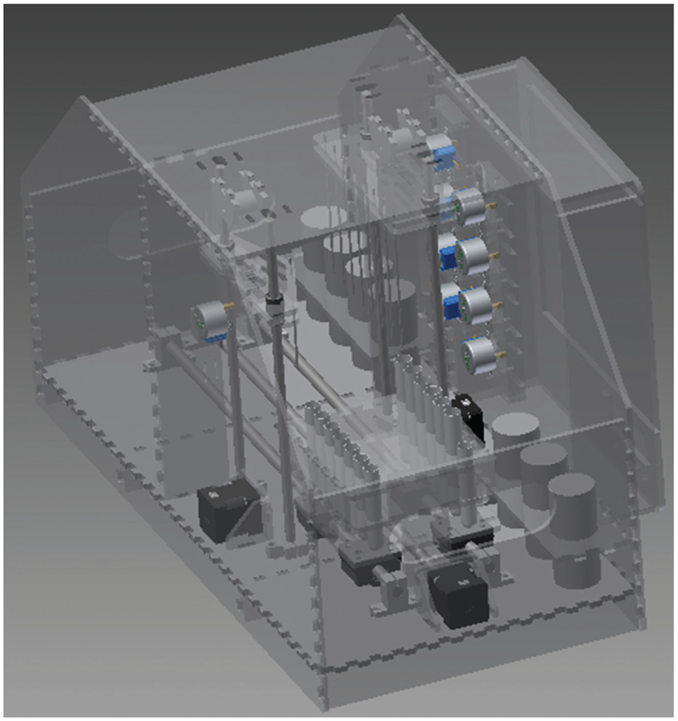
Computer-aided design of automated device in Autodesk Inventor 2015.
Manufacture
All components were laser cut from 5 mm clear acrylic using an LS 6090 PRO Laser engraving and cutting machine (HPC Laser Ltd., West Yorkshire, UK) at Newcastle University School of Mechanical and Systems Engineering. Components were joined using standard acrylic adhesive. No special equipment is required for assembly. Three-dimensional printed components were manufactured by a local supplier from clear acrylonitrile butadiene styrene (ABS).
Motion
Steel linear shaft bars and greased bearings are used on all moving axes. Movement of components is controlled by National Electrical Manufacturers Association size 14 (NEMA 14) stepper motors. Heat from stepper motors is dispersed by convection and the system designed so heat does not dissipate to fluids, potentially altering their density.
Stepper motors are driven at speeds greater than those which were noted to cause vibration (vibration was noted with speeds less than 150 steps/min for NEMA 14 motors). Vibration could affect the gradient by causing mixing at the fluid layers. Furthermore, the horizontal stepper motor was used to drive a leadscrew with an additional inertial load. The leadscrew is an effective means of dampening stepper oscillations that can cause vibration. The A4988 stepper motor driver (see below) also allows for microstepping, which would further reduce vibration by limiting changes in inertia. This was not required, but can easily be applied by connecting microstep pins according to manufacturer guidelines, depending on the desired microstep resolution. Furthermore, rubber washers between stepper motors and acrylic could be applied if vibration became problematic.
Stepper motors are accelerated from stopped positions to minimum speeds to avoid step losses that might cause positional inaccuracy. Limit switches control movement boundaries and home stepper motor positioning. Movement relative to home positions is calibrated at setup to ensure accurate positioning.
Fluid Delivery
Low-flow-rate, positive displacement peristaltic pumps are designed to be stepper motor driven for delivery of precise volumes of fluid ( Fig. 4 ). Stepper motors are accelerated from stopped positions to initial delivery speeds to avoid step losses and ensure precision of volume delivery. Fluid is delivered at a slow initial flow rate and thereafter accelerated linearly. The result is a small cushion of fluid being delivered at a slow initial rate with negligible mixing between layers. Subsequent faster delivery minimizes delivery times without compromising layer integrity. Both these settings are adjustable by the user. A suggested starting rate for fluid delivery to minimize mixing is 0.4 mL/min, with a suggested maximum delivery rate of 1 mL/min. Widely available unipolar 5 V 28BYJ-48 stepper motors are used, with the common wire disconnected and driven using a bipolar stepper driver to increase torque. Heat from stepper motors is dispersed by convection. Stepper motors drive five bearing rotors that were 3D printed. Ball bearings are 5 mm internal diameter × 10 mm external diameter × 4 mm width, stainless steel, and rubber sealed. Tygon E-3603 laboratory tubing (1.6 mm internal diameter × 3.2 mm external diameter) is used for fluid delivery. Peristaltic pumps were designed to give a tubing compression of 15%. Tubing compression is the ratio of the minimum gap between pump wall and rotor bearing (point of maximum occlusion) to the combined tubing wall thickness. The greater the tubing compression ratio, the lower the likelihood of backflow, but this approach can reduce tubing life. To minimize fluid pulsations, an inevitable consequence of peristalsis, pump walls were designed with tapering of occlusion. Maximal occlusion occurs at top dead center. Fluid is dispensed to the coated ultracentrifuge tube walls from 1.6 mm external diameter × 1.4 mm internal diameter brass tubing. The brass tubing is arranged to rest against ultracentrifuge tube walls, just above the upper border of the fluid meniscus from the previous fluid layer. This allows gentle delivery of fluid over the previous layer.
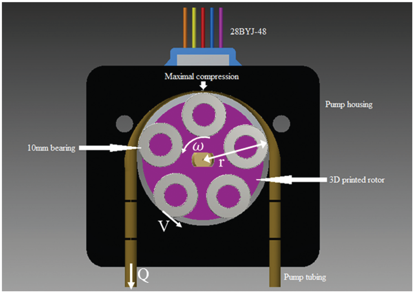
Peristaltic pump design. Symbols indicate expressions in equations 1-3.
Electronics
All electronic components were purchased either online or through Maplin Electronics (Rotherham, UK). Electronic circuitry was controlled from a 5 V Arduino Mega 2560 Board. A4988 bipolar stepper motor drivers were used in full-step operation to drive all stepper motors at 9 V, including the peristaltic pumps. Drivers are mounted on a custom printed circuit board (PCB) and current limited according to manufacturer specifications. At rest, NEMA 14 stepper motors were current limited to 0.5 A per coil, and 28BYJ-48 stepper motors to 0.23A per coil. PCBs are designed using Fritzing (fritzing.org) with traces transferred by laser toner transfer method and etched using ferric chloride. NEMA 14 stepper motors are connected to drivers using category 5e cabling. A 16 × 2 character backlit liquid crystal display (LCD) and four-button user input are mounted on a separate PCB.
A fluid level detector was placed at station 8 to ensure the total volume of fluid delivered to each test tube was precisely regulated ( Fig. 5 ). The detector consisted of a second brass rod that was vertically aligned with the brass delivery tubing and electrically isolated from it. The tip was horizontally aligned with the delivery tube and signal lines soldered to each. Fluid was detected when the tips of both brass rods were immersed in the uppermost salt-containing solution, completing the circuit. The detector can be enabled or disabled via the LCD software menu (Setup → Fluid level). The fluid level detector could be disabled if there was a significant variation in test tube radii, which would result in inconsistent volumes of fluid in tubes at the same total height.
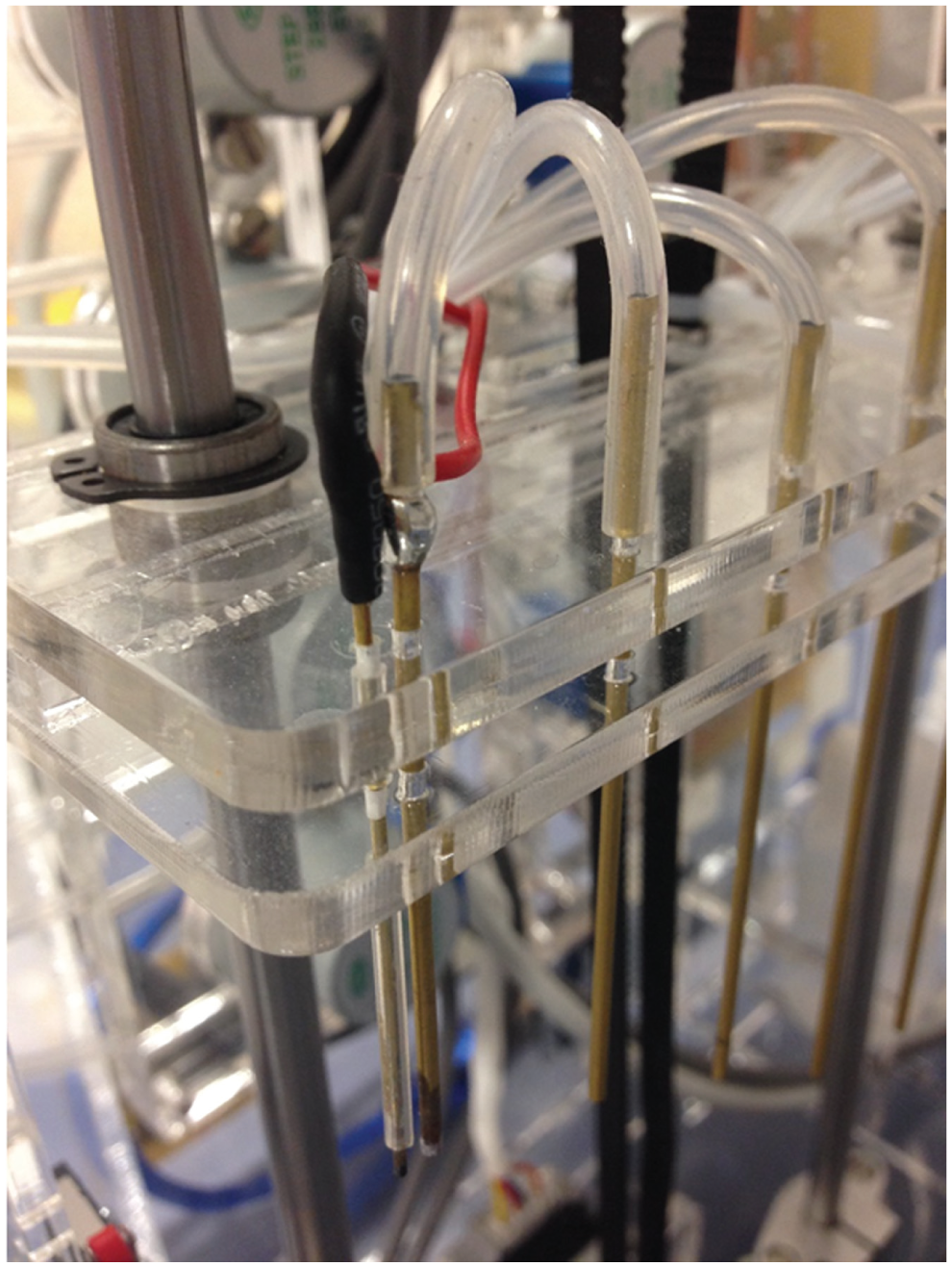
Fluid detector for ensuring total height (and therefore volume) of fluid delivered to each test tube remains constant.
Signal lines are connected to switches using shielded twisted pair cable with shield connected to ground. Power for the whole device is provided by a 9 V, 54 W medical power supply (RS Components, Corby, UK). Current draw with stepper motors at rest (maximal) is 5 A.
Software
All software is written in C++ using Microsoft Visual Studio with Visual Micro add-in (http://www.visualmicro.com/). Software is coded to ensure stepper motor motion is smooth, without delay, accurate, and reproducible. User set calibration values are added to ensure brass fluid delivery tubes are precisely positioned and fluid delivery volume accurate.
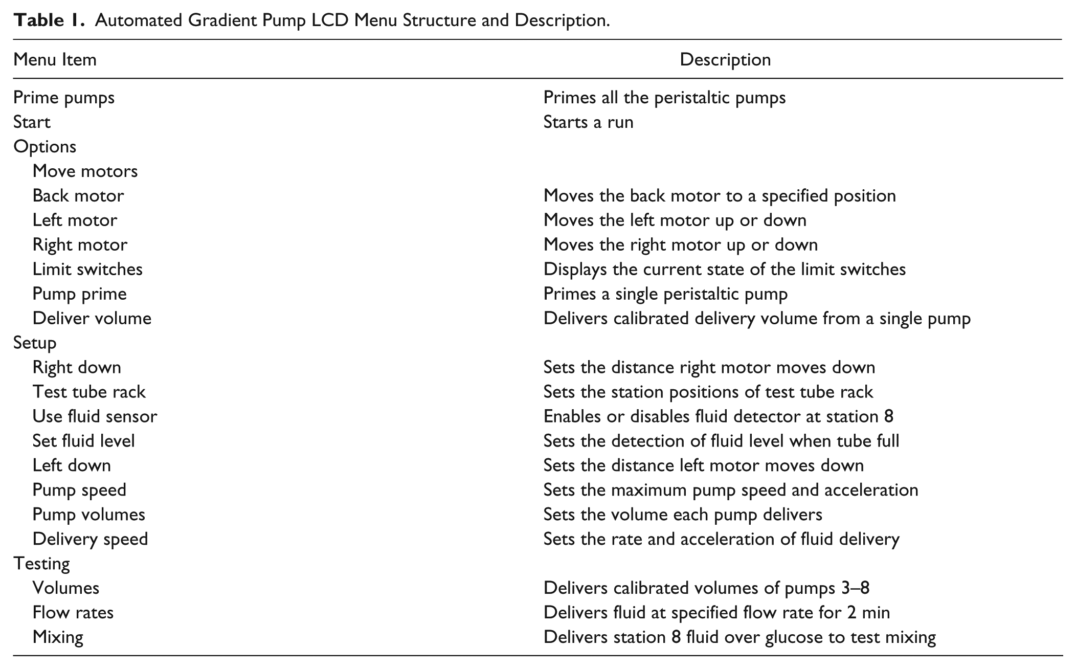
Stepper motor acceleration is performed using the AccelStepper library (http://www.airspayce.com/mikem/arduino/AccelStepper), available for use under the GNU General Public License (http://www.gnu.org/copyleft/gpl.html). The library has been modified for use with peristaltic pumps. An LCD menu structure ( Table 1 ) is created using the MenuBackend library (https://github.com/WiringProject/Wiring/tree/master/framework/libraries/MenuBackend), also available under the GNU GPL. All signal lines are software denounced using a debounce time constant of 50 ms.
Automated Gradient Pump LCD Menu Structure and Description.
Results and Discussion
Evaluation
The performance of the device was evaluated by testing under standard laboratory conditions and compared to previous usual practice, assessed under identical conditions. All weights were measured using a calibrated precision AL204 analytical balance (Mettler Toledo, Leicester, UK).
Density solutions were prepared from measured combinations of stock solutions. Stock solutions were prepared in volumetric flasks and consisted of 1003 mL 18 MΩ ultrapure deionized water combined with 11.4 g sodium chloride (density 1.006 g/mL), and sodium bromide in 0.195 M sodium chloride (density 1.182 g/mL). Stock solutions contain 0.001% disodium ethylenediaminetetraacetic acid (Na2 EDTA) and densities confirmed to within 0.001 g/mL of specified values. For the purpose of evaluation, human plasma was replaced with 1.006 g/mL sodium chloride stock solution. Two-milliliter samples were adjusted to density 1.118 g/mL by the addition of 0.341 g sodium chloride.
Usual practice consisted of measuring aliquots of density-adjusted sodium bromide solutions (1.182 g/mL [0.5 mL], 1.0988 g/mL [1 mL], 1.0860 g/mL [1 mL], 1.0790 g/mL [2 mL], 1.0722 g/mL [2 mL], 1.0641 g/mL [2 mL], 1.0588 g/mL [2 mL]) into vials using a calibrated pipette (PIPETMAN Classic, Gilson Scientific Ltd., Bedfordshire, UK). Density gradients were formed in polyvinyl alcohol–coated clear ultracentrifuge tubes (7301W UltraCote tubes, Seton Scientific, Los Gatos, CA). Solutions were transferred using a BT100M peristaltic pump (Baoding Shenchen Precision Pump Co. Ltd., Baoding, China). Tygon E-3603 laboratory tubing (1.6 mm internal diameter; Cole-Parmer Instrument Company, London, UK) was connected to 2 mm external diameter borosilicate glass capillary tubes (Capillary Tube Supplies, Cornwall, UK). The solutions were delivered carefully against the coated test tube walls, requiring considerable dexterity from the operator.
Statistical Analysis
Statistical analyses were performed using Minitab 16.0 Statistical software (Minitab Ltd., Coventry, UK). Data are presented as mean (± standard deviation where indicated). Statistical comparisons between usual practice and the automated device were performed using a two-tailed Student’s t test. Statistical significance was accepted at p < 0.05. Correlation was calculated using Pearson correlation coefficient.
Assessment of pump flow rate precision and accuracy
Pump flow rates were confirmed by measurement of delivered fluid volumes over 2 min at varying pump speeds. Using deionized water, delivered fluid mass was measured using the analytical balance. Volume was calculated using a density of 0.9982 g/mL at 20°C. A total of 24 measurements at each pump speed were recorded. Pump flow rate precision was defined as the mean absolute relative differences of flow rates from the group sample mean, expressed as a percentage of the group sample mean. The pump flow rate precision for the usual-practice pump was ±1.4% and for the automated device was ±0.7%. The relationship between pump speed and flow rate was determined by linear regression ( Fig. 6 ) with a coefficient of determination, r2 = 0.99 for both devices. Pump flow rate accuracy was defined as the absolute relative difference of the group sample means from the calculated flow rate derived from linear regression, expressed as a percentage of the calculated flow rate. The pump flow rate accuracy was ±2.7% for the usual-practice pump and ±5.5% for the automated device. These results demonstrate that pump flow rates can be precisely delivered using simple cost-effective peristaltic pumps. Flow rate accuracy was expected to be lower as pumps are driven by individual stepper motors on the automated device compared to a single stepper motor on the multichannel BT100M peristaltic pump. This meant any slight variation between individual stepper gearing ratios would be apparent as a reduction in accuracy. In practical terms, the variation of actual from calculated flow rates would not be significant, as the small difference would not have any significant effect on layer mixing and the required delivered volume is not uniquely dependent upon flow rate.
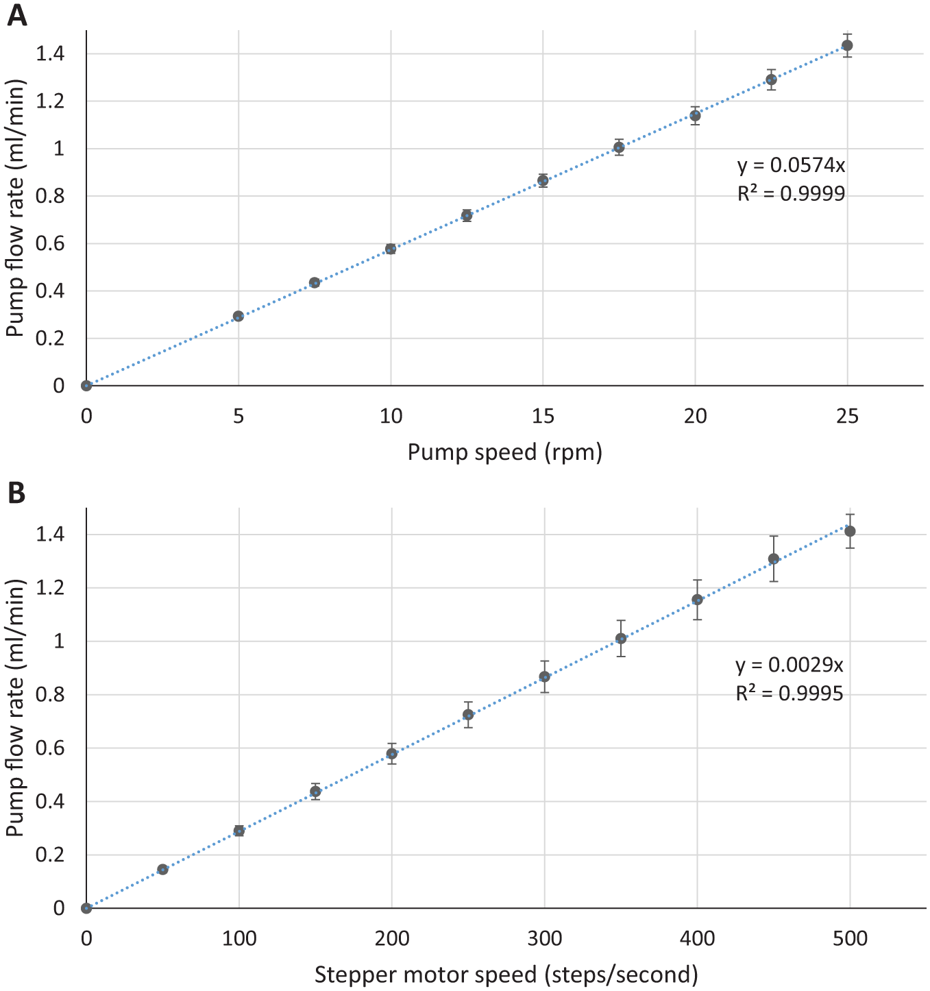
Mean (± standard deviation) flow rates for (
An estimate of fluid delivery flow rate can also be calculated using the design characteristics of the pump and compared to the results measured above, as noted below.
The velocity of fluid through the tubing is determined by the velocity of movement of the bearings along the tubing. The linear velocity V (mm/s) of the bearings along the tubing can be calculated by the following equation:
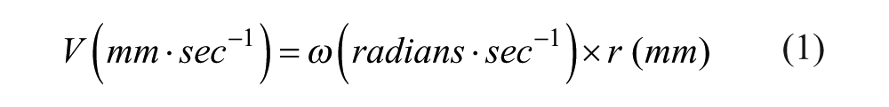
where
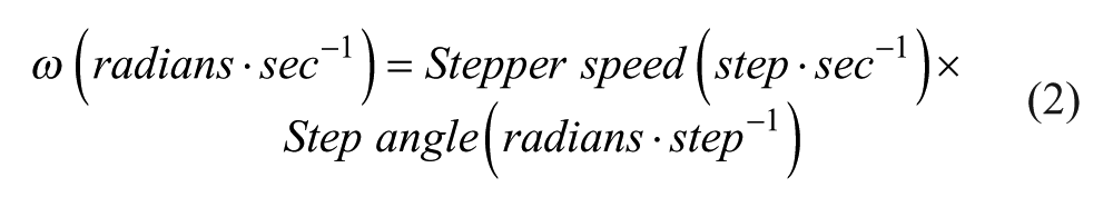
The 28BYJ-48 stepper motor has a step angle of 5.625° and a gearing ratio of 1:64, giving a shaft rotation angle of 5.625/64° per step. Degrees are converted to radians by multiplying by 2π/360. The rotor is attached directly to the shaft and therefore turns through the same angle.
The volumetric flow rate of fluid through the tubing is calculated as follows:
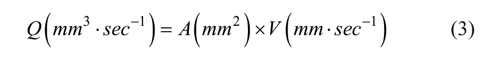
where V is the average linear velocity of fluid through the tubing from eq 1 and A the cross-sectional area of the inner tubing. The internal diameter of the tubing used was 1.6 mm. Flow rate can be converted to milliliters per minute by multiplying by 60 (s/min) and dividing by 1000 (mL/mm3).
Substituting and solving for eq 3 gives a final calculation:
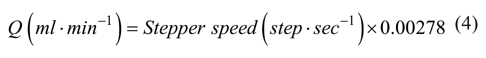
Comparison with the calculated linear slope coefficient from the measured flow rates above ( Fig. 6 ) shows calculated flow rates would lie within 3.5% of measured flow rates. Flow rates can therefore be reasonably estimated from the design characteristics of the pump, without having to be subjected to rigorous testing procedures.
Assessment of accuracy and precision of delivered volumes
Accuracy and precision of fluid volumes delivered by pumps were measured using a calibrated analytical balance. Usual practice consisted of measuring 1 mL aliquots of deionized water into vials using a calibrated pipette (PIPETMAN Classic, Gilson Scientific Ltd.). Solutions were then transferred to ultracentrifuge tubes using the BT100M peristaltic pump. Automated practice consisted of automated delivery of calibrated volumes into ultracentrifuge tubes. After filling the tubes, final weight was recorded and subtracted from tube weight to calculate weight of fluid delivered. Accuracy was defined as the mean absolute relative difference from the target weight, expressed as a percentage of the target weight. Accuracy of volume of fluid delivered was 0.7% by usual practice and 1.0% for the automated device. Precision was defined as the mean absolute relative weight difference from the group sample mean, expressed as a percentage of the group sample mean. Precision of volume of fluid delivered was 1.8% by usual practice and 0.8% for the automated device. These results demonstrate that calibrated stepper motor–driven peristaltic pumps can deliver fluid volumes with the required accuracy and precision by the automated method.
Assessment of layer mixing
In order to assess the degree of mixing at the layers upon fluid delivery, we devised a technique to quantify it. The final layer of the density gradient consists of a cushion of 1.0641 g/mL solution under 1.0588 g/mL sodium bromide solution. This layer has the smallest difference between solution densities and therefore is the most prone to mixing; hence, this layer was chosen for evaluation. Ten percent glucose solution (Fresenius Kabi, Cheshire, UK) containing 0.001% Na2 EDTA was adjusted to density 1.0641 g/mL by the addition of sodium bromide. This was overlayered with 2 mL 1.0588 g/mL sodium bromide solution by either peristaltic pump (usual practice) or automated device. Pump flow rates were matched between groups. The top 2 mL was aspirated using glass Pasteur pipettes, with tips drawn out under a flame to a fine point. By narrowing the tip, tiny quantities of fluid could be drawn from the surface accurately. Aspirated volume was confirmed by weight using an analytical balance. Glucose was measured on the aspirated volume using the glucose oxidase method on an YSI 2300 glucose analyzer (YSI [UK] Ltd., Hampshire, UK). Percentage mixing was calculated as the ratio of glucose concentration in the aspirated supernatant to the glucose concentration in the 10% glucose infranatant. The molecular weight of
Mean percentage mixing of layers was 5.9% for usual practice and 4.1% for the automated device (absolute percentage difference 1.8%, p = 0.001) ( Fig. 7 ). This represents a statistically significant reduction in fluid mixing, which is of utmost importance in gradient formation. These results also represent best practice, as every care and attention was being taken during usual-practice gradient formation to definitively avoid layer mixing. It is highly likely that in real-world usual practice, layer mixing would be greater than the 5.9% achieved in this study.
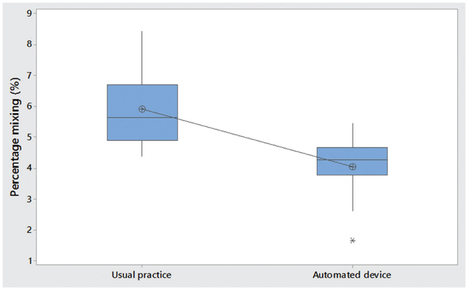
Boxplot of percentage layer mixing by usual practice and automated device.
Assessment of laboratory staff labor time
A sample of five measurements of time taken to complete formation of the density gradient in six tubes by usual practice showed a mean standard time to completion of 28 min (standard deviation 1 min, 48 s). The time to complete formation of the density gradient by the automated device was 32 min, and is constant as it is completely automated (unless delivery flow rate or acceleration is adjusted, increasing either will decrease time taken or vice versa). As the process requires no staff input and can be left to complete a cycle, this saves 28 min of laboratory technician time.
Cost analysis
The cost (USD) of producing a finished device was assessed from the component costs and approximate technician time to assemble and calibrate the systems. This was estimated to be $250 for mechanical components and $228 for electrical components. Technician time for assembly was estimated at 20 h, and based on an hourly rate of $43 per hour, gives an estimated cost of $860. 9 Given the relatively low cost of components, the technician time becomes dominant. The total estimated cost of producing the device is therefore $1338.
Comparing the time saved when using this automated system (28 min) and based on the same estimated hourly rate above, the device will pay for itself after approximately 31 h of operation (66 operations). The planned use for our institution greatly exceeds this, making it a financially viable and attractive solution.
In conclusion, we have developed an automated solution for creating density gradients suitable for separation of lipoproteins by zonal ultracentrifugation. The system is simple and can be easily manufactured with equipment that is readily available. It uses common components that can be purchased easily online, and the plans and software are available for free download. The system saves significant laboratory technician time and results in an accurate and reliable delivery of fluid in a preprogrammed and flexible fashion, as it can be readily modified to accommodate future requirements. Using the device also results in a significant reduction of mixing between the density layers, which is of vital importance to maintaining the integrity of the gradient for accurate separation of lipoproteins.
Footnotes
Acknowledgements
We thank Frank Atkinson from the Newcastle University School of Mechanical and Systems Engineering for his assistance in the construction of materials and Chris Morton from the Newcastle University School of Electrical and Electronic Engineering for his assistance in electrical design and testing. We also wish to thank the staff of the Newcastle Magnetic Resonance Centre, where the device was evaluated.
Declaration of Conflicting Interests
The authors declared no potential conflicts of interest with respect to the research, authorship, and/or publication of this article.
Funding
The authors disclosed receipt of the following financial support for the research, authorship, and/or publication of this article: All materials were purchased by the author (C.N.P.) or donated by the Newcastle University School of Mechanical and Systems Engineering.