Modeling Mass Transfer from Carmustine-Loaded Polymeric Implants for Malignant Gliomas

Abstract

Significant advances in the encapsulation and release of drugs from degradable polymers have led to the Food and Drug Administration approval of Gliadel wafers for controlled local delivery of the chemotherapeutic drug carmustine to high-grade gliomas following surgical resection. Due to the localized nature of the delivery method, no pharmacokinetic measurements have been taken in humans. Rather, pharmacokinetic studies in animals and associated modeling have indicated the capability of carmustine to be delivered in high concentrations within millimeters from the implant site over approximately 5 days. Mathematical models have indicated that diffusion has a primary role in transport, which may be complemented by enhanced fluid convection from postsurgical edema in the initial 3 days following implantation. Carmustine’s penetration distance is also presumably limited by its lipophilicity and permeability in the capillaries. This review discusses the mathematical models that have been used to predict the release and distribution of carmustine from a polymeric implant. These models provide a theoretical framework for greater understanding of systems for localized drug delivery while highlighting factors that should be considered in clinical applications. In effect, Gliadel wafers and similar drug delivery implants can be optimized with reduction in required time and resources with such a quantitative and integrative approach.

Introduction

Malignant gliomas (glioblastoma multiforme, anaplastic astrocytoma, anaplastic oligoastrocytoma, and anaplastic oligodendroglioma) are classified as World Health Organization grade III or IV cancers. ¹ These gliomas are generally diagnosed by cranial magnetic resonance imaging (MRI) or with computed tomography (CT) scans in combination with biopsies. The common treatment strategy against brain tumors is a combination of surgical removal, chemotherapy, and radiotherapy. ² Despite the combination of treatment strategies, remnant tumors capable of proliferation often survive, leading to tumor recurrence. Ninety percent of these recurrences occur within 2 cm of the original resection site. ³ In effect, the prognosis for patients with malignant gliomas is poor with a median survival of less than 2 years. ⁴ Due to the consistently poor prognosis of this disease, there continues to be a great motivation to develop novel therapeutic approaches.

Carmustine (BCNU, 1,3-bis(2-chloroethyl)-1-nitrosourea) is an important lipophilic chemotherapeutic drug that treats brain tumors by alkylating DNA and inhibiting the further synthesis of DNA, RNA, and protein. However, intravenous perfusion of carmustine has had limited success due to several issues. First, it has a short half-life of about 20 min in plasma. Second, the blood-brain barrier (BBB) allows only a small fraction of the administered dose to reach the tumor site. ⁵ The BBB consists of tight capillary cellular junctions that restrict the entry of many drugs into the brain from the bloodstream. Only a few chemotherapeutic agents are able to reach the tumor target at cytotoxic concentrations through the intravenous route. While the lipophilicity of carmustine allows it to cross the BBB more effectively than other drugs, studies have shown that not enough of the drug actually reaches the tumor site. ⁶ Third, carmustine is prone to induce systemic toxicity to the central nervous system (CNS) and other organs. ⁷

Recent research has moved toward the use of polymeric implants for controlled local drug delivery as a solution to the problems of systemic delivery. In contrast with systemic delivery, local or interstitial delivery of chemotherapeutic drugs bypasses the BBB and allows for higher concentrations of drugs in the target area. The slow degradation of polymeric implants makes sustained delivery for extended periods possible. Interstitial delivery also limits the volume distribution of drug in the body, thereby avoiding toxic effects to other organs.

In 1996, the carmustine implant Gliadel was approved by the US Food and Drug Administration (FDA) as an effective local treatment for recurrent malignant glioma. ⁸ It is the first and currently the only available local drug delivery treatment of brain tumors with FDA approval. Gliadel wafers are composed of carmustine distributed homogeneously in Polifeprosan 20 (also denoted as p(CPP:SA)), a solid, random copolymer matrix of 1,3-bis-(p-carboxyphenoxy)propane (CPP) and sebacic acid (SA) in a 20:80 molar ratio. Each 200-mg wafer is loaded with 3.85% carmustine and measures 14 mm in diameter and 1 mm in thickness. Up to eight wafers (containing an approximate total of 60 mg of carmustine) are implanted along the walls of the resulting cavity following surgical resection of a tumor. As the wafers degrade, they deliver carmustine to the surrounding cells over the course of about 3 weeks. ⁴ A 2006 long-term trial reported that patients with malignant glioma treated with Gliadel wafers combined with radiotherapy had an extended survival of 2 to 3 years. ⁹ However, several recent studies also report that the implantation of Gliadel wafers does little to reduce recurrence.^10,11 As shown from these contradicting studies, there is much room for optimization and improvement of the carmustine delivery system and, in general, drug delivery from polymeric implants.

It is difficult to obtain accurate real-time and conclusive observations about the fates of delivered chemotherapeutics in the human brain without invasive operations. Therefore, mathematical models and simulations are essential to develop a better understanding of carmustine delivery from implantable wafers. General models of drug delivery from polymers that capture drug transport, elimination, and binding have been applied to the specific case of carmustine delivered to the brain interstitium. This review aims to provide a comprehensive review of existing mathematical models and simulations of carmustine release from polymers and of its transport into adjacent tissue. To this end, this article begins with an extensive review of 1D studies in animal models and transitions to advanced 3D computer simulations. This review also discusses the factors that should be considered and optimized for future human applications in the clinical setting.

Modeling Drug Release

Drug Release from a Monolithic Sphere

Drug release from a polymeric system may involve several different processes, including drug diffusion, drug dissolution, and matrix erosion. ¹² Carmustine dispersed within a Polifeprosan 20 matrix can be described by the diffusional release model from a monolithic system as described by Ritger and Peppas. ¹³ By definition, a monolithic system is characterized by homogeneous distribution of the drug throughout the polymer matrix. In this model, the following assumptions are considered:

• The initial concentration of drug is lower than the solubility of the drug in the polymer.

• Diffusional mass transport of the drug is release-rate limiting and 1D.

• The effective diffusion coefficient (diffusivity) of the drug is constant.

• The surface drug concentration is kept at a constant concentration during the period of study.

• There is negligible swelling or erosion of the polymeric device.

• The drug is much smaller than the thickness of the polymer membrane.

In the case of 1D release in the radial direction from a sphere, the polymer release rate of carmustine has been derived to be

$$\frac{M_t}{M_{\infty }}=6{\left[\frac{Dt}{a^2}\right]}^{1/2}\left[\frac{1}{\sqrt{\pi }}+2{\displaystyle \sum _{n=1}^{\infty }\text{ierfc}\left(\frac{na}{\sqrt{Dt}}\right)}\right]-3\frac{Dt}{a^2},$$

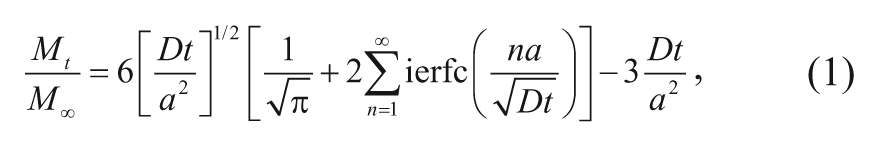
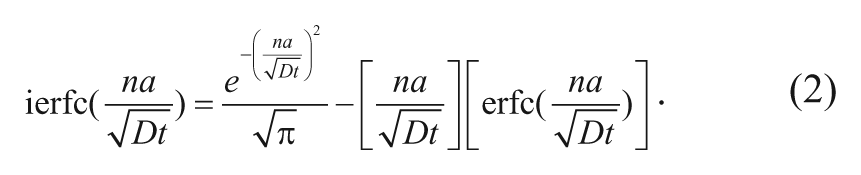
where M_∞ is the initial mass of carmustine in the polymer, M_t is the mass of carmustine released from the polymer at time t, a is the radius of the polymer, D is the effective diffusion coefficient of the drug in the polymeric matrix, and ierfc(x) represents the integrated complementary error function for x, which in this case is given by

$$\text{ierfc(}\frac{na}{\sqrt{Dt}})=\frac{e^{-{\left(\frac{na}{\sqrt{Dt}}\right)}^2}}{\sqrt{\pi }}-\left[\frac{na}{\sqrt{Dt}}\right]\left[\text{erfc(}\frac{na}{\sqrt{Dt}})\right].$$

When t is small, a “short time” approximation can be made that makes the first term and the complementary error function term in equation (2) equal to zero, reducing the entire integrated complementary error function to zero. Equation (1) therefore simplifies to

$$\frac{M_t}{M_{\infty }}=6{\left[\frac{Dt}{\pi a^2}\right]}^{1/2}-3\frac{Dt}{a^2}\text{for}\frac{M_t}{M_{\infty }}<\mathrm{0.40.}$$

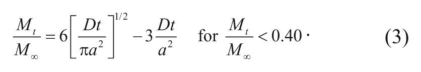
Graphical representation of the above equation demonstrated that the “short time” approximation is only valid during the first 40% of the fractional drug release. ¹⁴ Equation (3) was used by Fung and coworkers ¹⁵ to model carmustine release from polymer implants incubated in phosphate-buffered saline (PBS) at 37 °C and from rat brains.

Drug Release from a Monolithic Slab

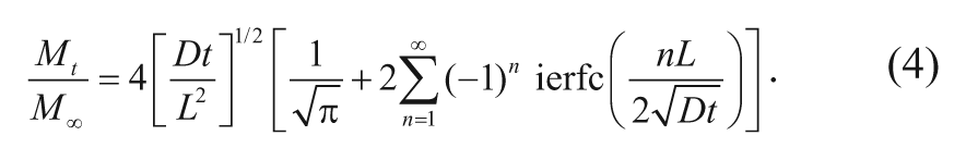
In the case of diffusion from a polymer slab with thickness L, the release rate of carmustine as a function of time has been derived as

$$\frac{M_t}{M_{\infty }}=4{\left[\frac{Dt}{L^2}\right]}^{1/2}\left[\frac{1}{\sqrt{\pi }}+2{\displaystyle \sum _{n=1}^{\infty }{(-1)}^n\text{ierfc}\left(\frac{nL}{2\sqrt{Dt}}\right)}\right].$$

In a manner similar to the spherical case, the short-time approximation simplifies equation (4) to the following expression:

$$\frac{M_t}{M_{\infty }}=4{\left[\frac{Dt}{\pi L^2}\right]}^{1/2}\text{for}\frac{M_t}{M_{\infty }}\le \mathrm{0.60.}$$

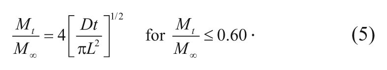
Graphical representation by Ritger and Peppas ¹³ demonstrated that equation (5) is only applicable up to the first 60% of fractional drug release.

As seen in the above equations, drug release by diffusion is characterized by a t^1/2 time dependence. Fung and coworkers ¹⁶ compared predictions from this model with their experiments on carmustine release from polymer disks incubated in PBS and noticed good correlation during the first day of incubation. The effective diffusion coefficient for transport through the polymer was empirically determined to be 6.7 × 10⁻¹⁰ cm²/s, a reasonable value for a small-molecule drug in Polifeprosan 20. Dang and coworkers ¹⁷ also noted that in vivo studies of carmustine release from normal rat brains showed a linear relationship between the cumulative drug release rate and the square root of time for approximately the first 10 h after implantation. In summary, the above equations can be applied to describe the drug release of carmustine from Gliadel wafers during early times when the drug is released primarily by diffusion through the polymer matrix. However, as the polymer erodes with time, the increasing porosity of the polymer facilitates carmustine release. Therefore, deviation from the models is evident at longer time spans.

One-Dimensional Mathematical Transport Models

Governing Equations for Drug Distribution in the Brain

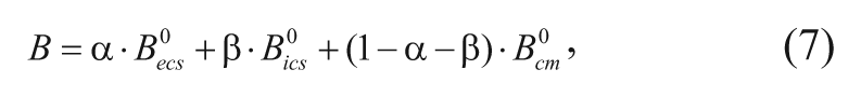
The brain can be divided into three phases: the interstitial/extracellular space (ECS), the intracellular space (ICS), and cellular membrane (CM). ¹⁸ Within the brain, the drug may be present in its unbound or bound form, where the latter is not subject to metabolism. ¹⁹ This presents a porous media-type problem, since it is fairly difficult to model the drug as it diffuses through the interstitial space of the brain. Instead, the brain is treated as a pseudo-one phase medium where the drug is assumed to freely diffuse throughout this entire pseudo-homogeneous phase. Hence, in this scenario, a differential sample of brain volume will include ECS, ICS, and CM. It is then appropriate to use a volume-averaging technique to describe the average concentration of drug in the brain. ¹⁸ The average concentrations of drug in both its free-floating and bound (immobilized) form are represented as follows:

$$C=\alpha \cdot C_{ecs}^0+\beta \cdot C_{ics}^0+(1-\alpha -\beta )\cdot C_{cm}^0,$$

$$B=\alpha \cdot B_{ecs}^0+\beta \cdot B_{ics}^0+(1-\alpha -\beta )\cdot B_{cm}^0,$$

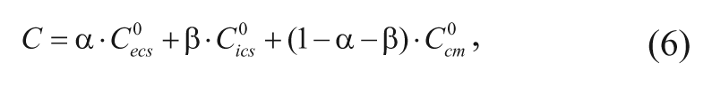
where C is the average free (unbound) drug concentration in the brain; $C_{ecs}^0$ , $C_{ics}^0$ , and $C_{cm}^0$ denote the free drug concentrations in the ECS, ICS, and CM phases, respectively; and α and β are volume fractions of the ECS and ICS, respectively. Similarly, the bound drug is defined analogously, where B is the average bound or internalized drug concentration in the brain; $B_{ecs}^0$ , $B_{ics}^0$ , and $B_{cm}^0$ denote the bound drug concentrations in the ECS, ICS, and CM phases, respectively; and α and β are the volume fractions of the ECS and ICS, respectively. The units of concentration are in moles per volume.

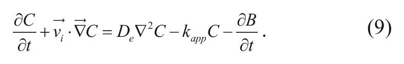
The multiple events that affect drug delivery from a carmustine implant can be captured in a governing equation characterizing drug distribution in the brain. The following method can also be applied to other polymeric drug release systems as well. Specifically, carmustine concentration in the brain depends on the rate of drug transport via convection and diffusion; elimination through degradation, metabolism, and blood capillary permeation; and local binding or internalization. Note that bound drug is assumed to be immobilized and unavailable for transport. ¹⁹ A mass balance on the drug gives the most general equation describing drug transport and elimination in the region near the polymeric implant ²⁰ :

$$\frac{\partial C}{\partial t}+\overrightarrow{v_i}\cdot \overrightarrow{\nabla }C=D_e{\nabla }^{2}C-R_e-\frac{\partial B}{\partial t},$$

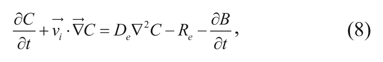
where t is time after implantation, $\overrightarrow{v_i}$ is the interstitial fluid velocity in the brain, and D_e is the effective diffusion coefficient of the drug in the tissue. The effective diffusivity must be used instead of the bulk diffusivity, since the drug is assumed to freely diffuse throughout the entire volume of the brain when in reality the entire volume is not entirely accessible. It also takes into account the tortuosity and varying cross-sectional area of the extracellular channels of the brain. The R_e term quantifies the total elimination and degradation of drug per unit volume. Since the brain is modeled as a rigid porous medium, the reaction term must be converted from a heterogeneous reaction to a homogeneous one. Usually, this is done by multiplying the original heterogeneous reaction term by a constant that considers the internal surface area of the porous medium per volume of the brain. However, for all of these models being reviewed, this is not explicitly done even though elimination and degradation are assumed to be homogeneous within the brain tissue.

Often, drug elimination and degradation are represented as a lumped first-order reaction that captures the behavior of several processes. Models have had lumped first-order reactions that incorporate the permeability of the BBB, elimination due to nonenzymatic reactions, or even enzymatic reactions that simplify the Michaelis-Menten equation to the first-order regime by assuming low concentrations of drug in the brain.^2,20 First-order approximations are used, since the concentration of drug in the tissue is assumed to be low and the drug concentration in blood plasma is much less than that in the tissue.^20,21 Equation (8) can therefore be rewritten with a generalized apparent first-order rate constant, or k_app, as follows:

$$\frac{\partial C}{\partial t}+\overrightarrow{v_i}\cdot \overrightarrow{\nabla }C=D_e{\nabla }^{2}C-k_{app}C-\frac{\partial B}{\partial t}.$$

In this case, the model does not include any receptor-associated reaction rate constants. This is unnecessary as carmustine is a small-molecule drug that can diffuse across cell membranes without the aid of a surface receptor. Carmustine passively diffuses across the cell membrane on its own or actively via a transporter. ²⁰ Alternatively, an equilibrium binding constant, defined as K_bind, is incorporated into the mass conservation equation. This relates the amount of bound drug to the amount of free-floating drug and will be further elaborated on in this review. In addition, note that the $\partial B/\partial t$ term is subtracted from the right side of the equation since any decrease in the rate of change of bound drug corresponds to an increase in concentration of unbound drug. In other words, any drug that is not bound in a phase must be free floating.

Fung and coworkers ¹⁵ have developed mathematical models describing local concentration profiles of carmustine and compared its values with experimental animal data. These models are based on diffusion of the drug both from a spherical pellet in rat brain and from a monolithic slab in monkey brain. They are derived by first substituting equations (6) and (7) into equation (9) and assuming that the elimination of drug proceeds by first-order processes:

$$\left[\begin{array}{l}\alpha \frac{\partial C_{ecs}^0}{\partial t}+\beta \frac{\partial C_{ics}^0}{\partial t}+(1-\alpha -\beta )\frac{\partial C_{cm}^0}{\partial t}+\\ \overrightarrow{v_i}\cdot \overrightarrow{\nabla }\left(\alpha C_{ecs}^0+\beta C_{ics}^0+(1-\alpha -\beta )C_{cm}^0\right)\end{array}\right]=\left[\begin{array}{c}{D}_e{\nabla }^2\left(\alpha C_{ecs}^0+\beta C_{ics}^0+(1-\alpha -\beta )C_{cm}^0\right)\\ -(\alpha \cdot k_{ecs}{C}_{ecs}^0+\beta \cdot k_{ics}{C}_{ics}^0+(1-\alpha -\beta )k_{cm}{C}_{cm}^0)\\ -\left(\alpha \frac{\partial B_{ecs}^0}{\partial t}+\beta \frac{\partial B_{ics}^0}{\partial t}+(1-\alpha -\beta )\frac{\partial B_{cm}^0}{\partial t}\right)\end{array}\right],$$

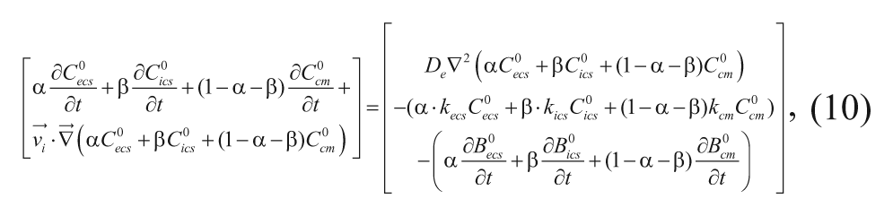
where k_ecs, k_ics, and k_cm are the first-order elimination constants of carmustine in the respective phases. Drug transportation occurs primarily through the ECS, ²⁰ eliminating the need to include $C_{ics}^0$ and $C_{cm}^0$ into the diffusion and convection terms in equation (10). Moreover, carmustine is assumed to be neither bound nor eliminated in the cell membrane. With this assumption, $k_{cm}=0$ and $B_{cm}^0=0$ , making the presence of bound drug and carmustine elimination significant only in the ECS and ICS phases. Applying these two assumptions to equation (10), Fung and coworkers ¹⁵ quantified transport and elimination in the brain with the following equation:

$$\begin{array}{l}\alpha \frac{\partial C_{ecs}^0}{\partial t}+\beta \frac{\partial C_{ics}^0}{\partial t}+(1-\alpha -\beta )\frac{\partial C_{cm}^0}{\partial t}+\overrightarrow{v_i}\cdot \overrightarrow{\nabla }\left(\alpha C_{ecs}^0\right)=\\ D_{ecs}{\nabla }^2\left(\alpha C_{ecs}^0\right)-(\alpha \cdot k_{ecs}{C}_{ecs}^0+\beta \cdot k_{ics}{C}_{ics}^0)-\left(\alpha \frac{\partial B_{ecs}^0}{\partial t}+\beta \frac{\partial B_{ics}^0}{\partial t}\right).\end{array}$$

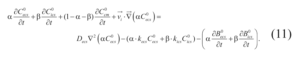
We will first focus on simplifying and solving equation (11) in spherical coordinates.

Spherical Geometry

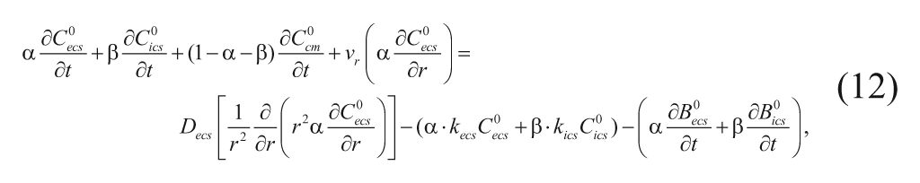
The radial, 1D equations written and solved by Fung and coworkers ¹⁵ describe the local concentration profiles of carmustine based on diffusion of the drug from a monolithic spherical pellet. Although the actual polymeric pellet implanted inside the rat brain in vivo was a small cylinder, Fung and coworkers modeled it as a sphere to simplify the mathematics. In this model, the drug diffuses from a spherically symmetric pellet into the pseudo-homogeneous medium of the brain. The adjacent brain tissue near the implant is similarly modeled as a sphere, as seen in Figure 1 . If the adjacent brain tissue is assumed to be isotropic, the concentration of drug will have no variation in the θ and ϕ directions. Accordingly, the drug conservation equation for a system dependent on only radial diffusion can be reduced from equation (11) to be as follows:

$$\begin{array}{l}\alpha \frac{\partial C_{ecs}^0}{\partial t}+\beta \frac{\partial C_{ics}^0}{\partial t}+(1-\alpha -\beta )\frac{\partial C_{cm}^0}{\partial t}+v_r\left(\alpha \frac{\partial C_{ecs}^0}{\partial r}\right)=\\ D_{ecs}\left[\frac{1}{r^2}\frac{\partial }{\partial r}\left(r^2\alpha \frac{\partial C_{ecs}^0}{\partial r}\right)\right]-(\alpha \cdot k_{ecs}{C}_{ecs}^0+\beta \cdot k_{ics}{C}_{ics}^0)-\left(\alpha \frac{\partial B_{ecs}^0}{\partial t}+\beta \frac{\partial B_{ics}^0}{\partial t}\right),\end{array}$$

Figure 1.

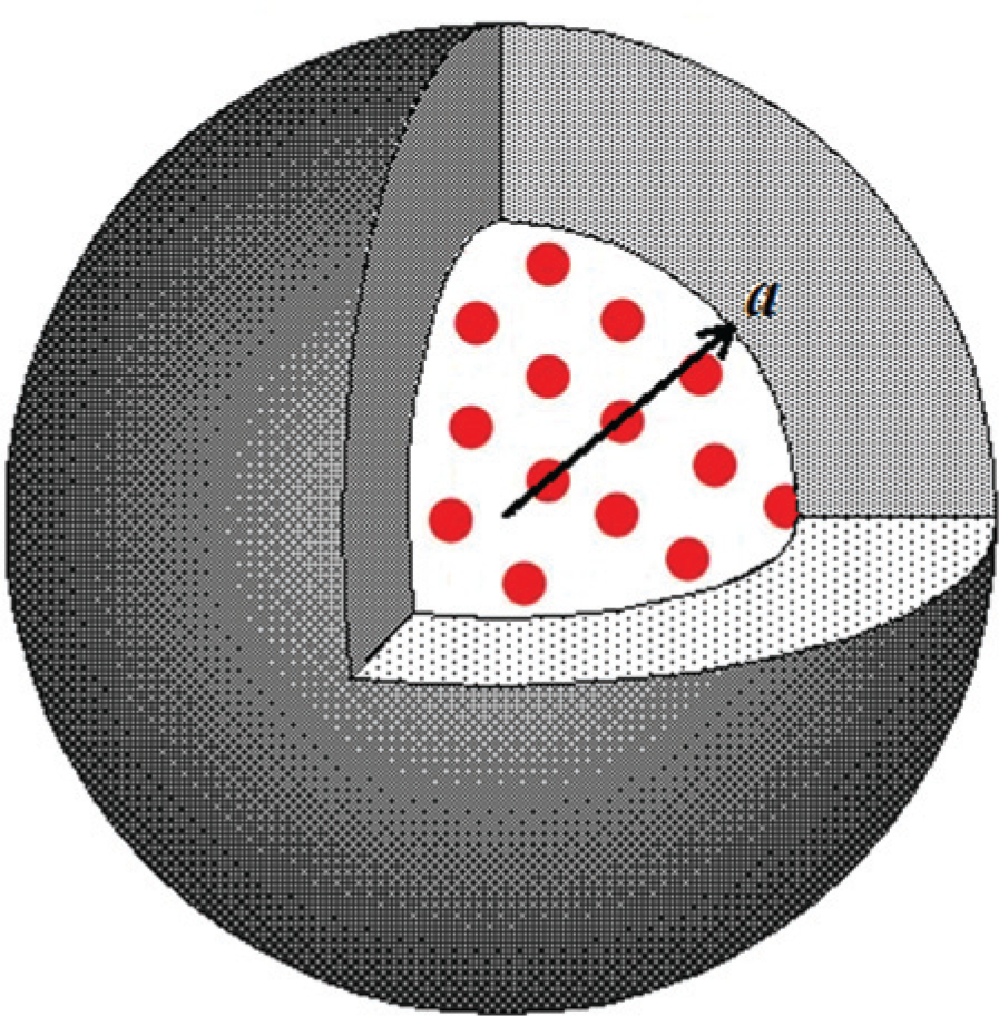
Schematic diagram demonstrating 1D radial diffusion of carmustine. The inner sphere portrays the monolithic pellet with radius a. Carmustine penetrates the adjacent pseudo-homogeneous brain tissue, represented by the outer sphere.

where r is the radial distance from the center of the spherical pellet, $v_r$ is the interstitial velocity in the radial direction, and D_ecs is the diffusivity of carmustine in the ECS.

To further simplify equation (12), a few more assumptions can be made to allow the equation to be completely written in terms of $C_{ecs}^0$ , making the total drug concentration proportional to the concentration in the ECS phase. As previously discussed, the concentration of bound drug is assumed to be directly proportional to the concentration of unbound drug. Accordingly, the concentration of bound carmustine is proportional to unbound carmustine in the ECS and ICS, while no drug is considered to be present in the CM phase. This assumption allows for the bound and unbound drug concentrations to be directly related using the binding constant K_ecs between bound and free carmustine in the ECS, as well as the binding constant K_ics between bound and free carmustine in the ICS.

$$K_{ecs}=\frac{B_{ecs}^0}{C_{ecs}^0},$$

$$K_{ics}=\frac{B_{ics}^0}{C_{ics}^0}.$$

Subsequently, the binding constants allow the concentration of the bound drug to be redefined in terms of free-floating drug as follows:

$$B_{ecs}^0=K_{ecs}{C}_{ecs}^0,$$

$$B_{ics}^0=K_{ics}{C}_{ics}^0.$$

Last, the free drug in the three phases is assumed to be in local equilibrium. This assumption is reasonable since the characteristic time for carmustine diffusion through the ECS is much greater than the characteristic time for the drug to permeate through cell membranes. ¹⁵ This means that the partitioning of the drug between phases can be related by the following partition coefficients:

$$P_{i:e}=\frac{C_{ics}^0}{C_{ecs}^0},$$

$$P_{m:e}=\frac{C_{cm}^0}{C_{ecs}^0},$$

where P_i:e is the partition coefficient between the ICS and ECS, and P_m:e is the partition coefficient between the CM and ECS. The concentration of unbound drug in the ICS and CM can then be related to the concentration of unbound drug in the ECS as follows:

$$C_{ics}^0=P_{i:e}{C}_{ecs}^0,$$

$$C_{cm}^0=P_{m:e}{C}_{ecs}^0.$$

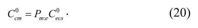
With these assumptions, equations (15) and (16) can be substituted for the concentration of unbound drug, along with equations (19) and (20) as new expressions for the concentration of free carmustine in the ICS and CM phases, into equation (12) to yield

$$\begin{array}{l}\alpha \frac{\partial C_{ecs}^0}{\partial t}+\beta P_{i:e}\frac{\partial C_{ecs}^0}{\partial t}+(1-\alpha -\beta )P_{m:e}\frac{\partial C_{ecs}^0}{\partial t}+v_r\left(\alpha \frac{\partial C_{ecs}^0}{\partial r}\right)=\\ D_{ecs}\left[\frac{1}{r^2}\frac{\partial }{\partial r}\left(r^2\alpha \frac{\partial C_{ecs}^0}{\partial r}\right)\right]-(\alpha \cdot k_{ecs}{C}_{ecs}^0+\beta P_{i:e}\cdot k_{ics}{C}_{ecs}^0)-\left(\alpha K_{ecs}\frac{\partial C_{ecs}^0}{\partial t}+\beta P_{i:e}{K}_{ics}\frac{\partial C_{ecs}^0}{\partial t}\right).\end{array}$$

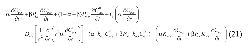
Combining like terms and rearranging simplifies equation (21) into

$$\begin{array}{l}(\alpha \cdot (1+K_{ecs})+\beta \cdot P_{i:e}\cdot (1+K_{ics})+(1-\alpha -\beta )\cdot P_{m:e})\frac{\partial C_{ecs}^0}{\partial t}+\alpha v_r\left(\frac{\partial C_{ecs}^0}{\partial r}\right)=\\ \alpha D_{ecs}\left[\frac{1}{r^2}\frac{\partial }{\partial r}\left(r^2\frac{\partial C_{ecs}^0}{\partial r}\right)\right]-(\alpha \cdot k_{ecs}+\beta P_{i:e}\cdot k_{ics})C_{ecs}^0.\end{array}$$

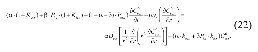
In addition, the collection of constants on the left can be defined as

$$\alpha *\equiv \alpha \cdot (1+K_{ecs})+\beta \cdot P_{i:e}\cdot (1+K_{ics})+(1-\alpha -\beta )\cdot P_{m:e}.$$

With the inclusion of this constant, equation (22) can be rewritten as

$$\alpha *\frac{\partial C_{ecs}^0}{\partial t}+\alpha v_r\left(\frac{\partial C_{ecs}^0}{\partial r}\right)=\alpha D_{ecs}\left[\frac{1}{r^2}\frac{\partial }{\partial r}\left(r^2\frac{\partial C_{ecs}^0}{\partial r}\right)\right]-(\alpha \cdot k_{ecs}+\beta P_{i:e}\cdot k_{ics})C_{ecs}^0.$$

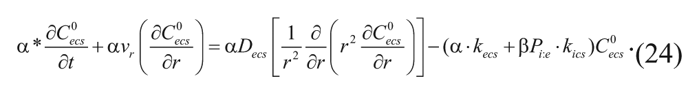
Dividing each term in equation (24) by $\alpha *$ yields

$$\frac{\partial C_{ecs}^0}{\partial t}+\frac{\alpha }{\alpha *}{v}_r\left(\frac{\partial C_{ecs}^0}{\partial r}\right)=\frac{\alpha }{\alpha *}{D}_{ecs}\left[\frac{1}{r^2}\frac{\partial }{\partial r}\left(r^2\frac{\partial C_{ecs}^0}{\partial r}\right)\right]-\frac{\alpha \cdot k_{ecs}+\beta P_{i:e}\cdot k_{ics}}{\alpha *}{C}_{ecs}^0.$$

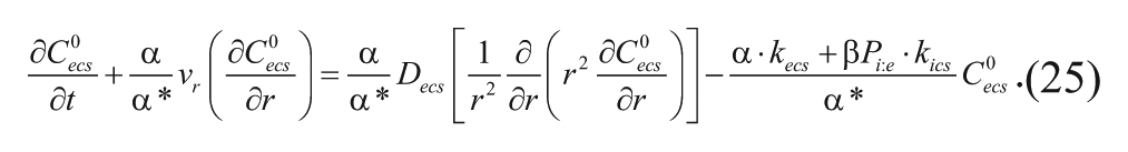
Furthermore, the apparent radial velocity, the apparent diffusivity, and the apparent first-order elimination can be defined, respectively, as follows:

$$v_{app}=v_r(\alpha /\alpha *),$$

$$D_{app}=D_{ecs}(\alpha /\alpha *),$$

$$k_{app}=(\alpha \cdot k_{ecs}+\beta P_{i:e}\cdot k_{ics})/\alpha *.$$

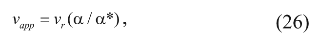
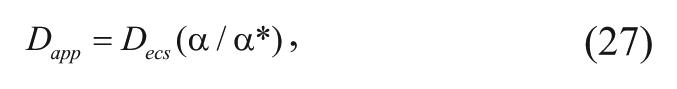
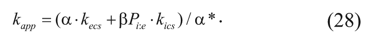
Using these definitions, equation (25) simplifies to the following equation:

$$\frac{\partial C_{ecs}^0}{\partial t}+v_{app}\frac{\partial C_{ecs}^0}{\partial r}=D_{app}\left[\frac{1}{r^2}\frac{\partial }{\partial r}\left(r^2\frac{\partial C_{ecs}^0}{\partial r}\right)\right]-k_{app}\cdot C_{ecs}^0.$$

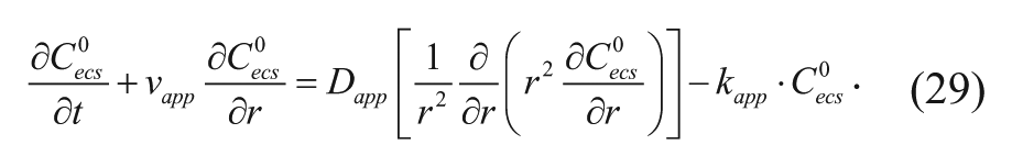
To write equation (29) in terms of the average total concentration C, the following algebraic operations will be performed. Substituting equations (19) and (20) into equation (6) yields

$$C=\alpha \cdot C_{ecs}^0+\beta \cdot P_{i:e}{C}_{ecs}^0+(1-\alpha -\beta )\cdot P_{m:e}{C}_{ecs}^0.$$

The $C_{ecs}^0$ term in equation (30) can be factored out, which yields

$$C=(\alpha +\beta \cdot P_{i:e}+(1-\alpha -\beta )\cdot P_{m:e})C_{ecs}^0.$$

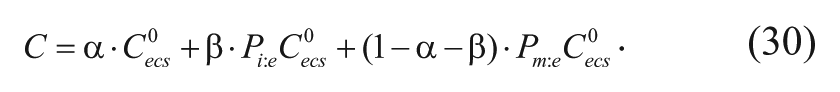
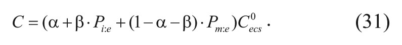
The summation of constants can then be defined accordingly:

$$\gamma \equiv \alpha +\beta \cdot P_{i:e}+(1-\alpha -\beta )\cdot P_{m:e}.$$

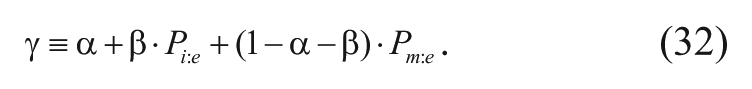
Subsequently, equation (31) can be rewritten with the new constant defined in equation (32) to yield

$$C=\gamma C_{ecs}^0.$$

Rearranging equation (33), the concentration of drug in the ECS phase can be related to the total average concentration as follows:

$$C_{ecs}^0=\frac{C}{\gamma }.$$

Substituting equation (34) into equation (29) yields

$$\frac{1}{\gamma }\frac{\partial C}{\partial t}+\frac{v_{app}}{\gamma }\frac{\partial C}{\partial r}=\frac{D_{app}}{\gamma }\left[\frac{1}{r^2}\frac{\partial }{\partial r}\left(r^2\frac{\partial C}{\partial r}\right)\right]-\frac{k_{app}}{\gamma }\cdot C.$$

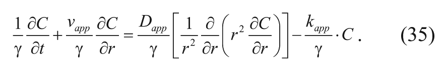
The γ term can be canceled out, thus allowing equation (35) to be reduced to the following equation:

$$\frac{\partial C}{\partial t}+v_{app}\frac{\partial C}{\partial r}=D_{app}\left[\frac{1}{r^2}\frac{\partial }{\partial r}\left(r^2\frac{\partial C}{\partial r}\right)\right]-k_{app}\cdot C.$$

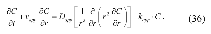
Equation (36), along with the initial and boundary conditions, can be used to study the behavior of the diffusing drug from the spherical implant. Fung and coworkers ¹⁵ solved this equation for situations with and without convection in healthy, nontumor brain tissue.

For the first case, convection of the drug is neglected, and the ν_app term is ignored. If steady-state conditions are assumed to be present, there is no time-varied concentration, and $\partial C/\partial t$ equals zero. Only two boundary conditions are needed to solve the problem: the pellet provides a sustained source of drug (equation (37)), and the concentration of the drug far from the implant is zero (equation (38)).

$$C=C_i\mathrm{for}t>0;r=a,$$

$$C=0\mathrm{for}t>0;r\to \infty .$$

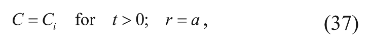
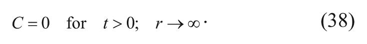
Applying the two boundary conditions after assuming steady state yields the following solution ¹⁵ :

$$\frac{C}{C_i}=\frac{a}{r}\exp \left[-\varphi \left(\frac{r}{a}-1\right)\right],$$

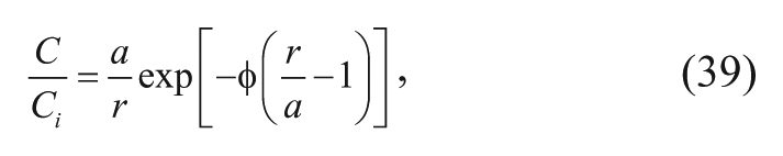
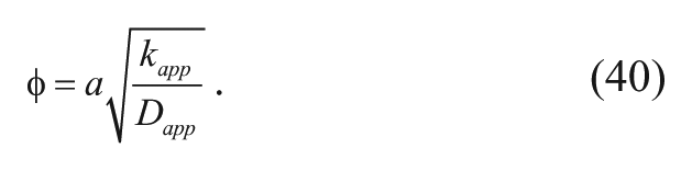
where C_i is the concentration of carmustine at the polymer-tissue interface, a is the radius of the spherical pellet, and φ the Thiele modulus that Fung and coworkers^15,16 refer to as the diffusion/elimination modulus. The Thiele modulus was derived (see Appendix A) as follows:

$$\varphi =a\sqrt{\frac{k_{app}}{D_{app}}}.$$

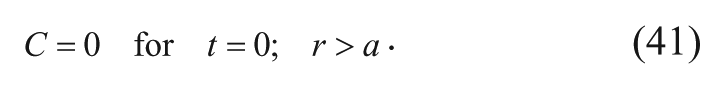
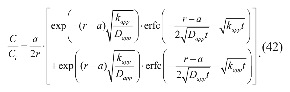
However, if the system is not at steady state, the concentration of drug is instead assumed to be zero outside the polymer pellet initially during surgical implantation.

$$C=0\mathrm{for}t=0;r>a.$$

Using equations (37), (38), and (41) as the boundary and initial conditions, the solution to the transient case with convection neglected for equation (36) is as follows ¹⁵ :

$$\frac{C}{C_i}=\frac{a}{2r}\cdot \left[\begin{array}{l}\exp \left(-(r-a)\sqrt{\frac{k_{app}}{D_{app}}}\right)\cdot \mathrm{erfc}\left(-\frac{r-a}{2\sqrt{D_{app}t}}-\sqrt{k_{app}t}\right)\\ +\exp \left((r-a)\sqrt{\frac{k_{app}}{D_{app}}}\right)\cdot \mathrm{erfc}\left(-\frac{r-a}{2\sqrt{D_{app}t}}-\sqrt{k_{app}t}\right)\end{array}\right].$$

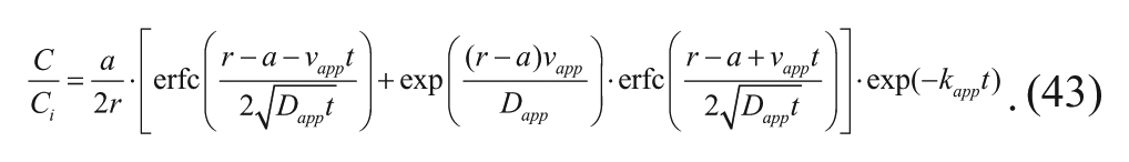
Alternatively, the transient case in which convection is included can be considered as well. Solving the governing equation without neglecting the velocity produces ¹⁵

$$\frac{C}{C_i}=\frac{a}{2r}\cdot \left[\mathrm{erfc}\left(\frac{r-a-v_{app}t}{2\sqrt{D_{app}t}}\right)+\exp \left(\frac{(r-a)v_{app}}{D_{app}}\right)\cdot \mathrm{erfc}\left(\frac{r-a+v_{app}t}{2\sqrt{D_{app}t}}\right)\right]\cdot \exp (-k_{app}t).$$

Fung and coworkers ¹⁵ used these equations to make predictions to compare with in vivo data from experiments in the rat brain. This is possible by using volume fraction values found in the literature and estimating the values for the partition coefficient, elimination constants, and binding constants, as well as using an empirically determined value for the diffusivity of carmustine. Depending on whether the solution was for the steady-state case or the transient case, the remaining parameters were adjusted to fit the experimental data. For the steady-state case, the data were fit to equation (39) to predict an experimental value of φ, which was subsequently compared with the Thiele modulus calculated from equation (40) using a value for the apparent elimination constant from the literature and an empirically determined diffusion constant for carmustine. For the transient case neglecting convection, the values for D_app and k_app in equation (42) were fitted to the experimental data, and these parameters were used to calculate φ. In both cases, the fitted value of the Thiele modulus was comparable to the Thiele modulus computed with the literature value for the apparent elimination constant and an empirically determined diffusivity. ¹⁵

Cartesian Coordinates

Fung and coworkers ¹⁶ extended their studies on polymeric drug distribution to the brains of monkeys. Mathematically, this case was modeled as 1D diffusion from a monolithic slab. Local drug concentrations were experimentally measured in serial coronal slices, which were cut perpendicularly relative to the drug-loaded polymer disk ( Fig. 2 ). ¹⁶

Figure 2.

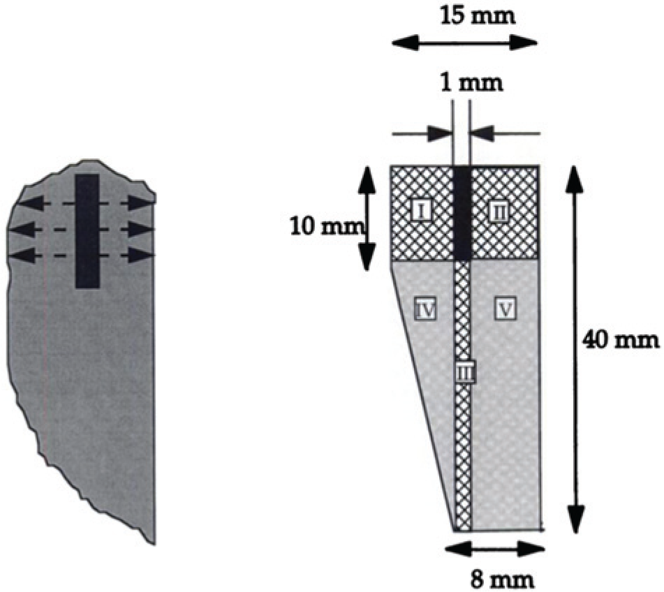
The illustration on the left describes coronal slices of the upper left portion of the monkey brain containing the perpendicularly implanted carmustine disk. Concentration profiles were measured normal to the surfaces of the monolithic slab with autoradiography. On the right is a schematic portrayal of the image on the left. These dimensions were used to determine the boundaries set in the mathematical model. Drug mass in sections I, II, and III were found to be much greater than sections IV and V. Reprinted from Fung et al. ¹⁶ with permission from American Association for Cancer Research.

Using the same assumptions as those employed for spherical coordinates, equation (11) can be simplified analogously in Cartesian coordinates. By substituting in equations (15), (16), (19), and (20) and assuming no variation along the y and z axes, the governing equation can be simplified to

$$\begin{array}{l}(\alpha \cdot (1+K_{ecs})+\beta \cdot P_{i:e}\cdot (1+K_{ics})+(1-\alpha -\beta )\cdot P_{m:e})\frac{\partial C_{ecs}^0}{\partial t}+\alpha v_x\left(\frac{\partial C_{ecs}^0}{\partial x}\right)=\\ \alpha D_{ecs}\left(\frac{{\partial }^2{C}_{ecs}^0}{\partial x^2}\right)-(\alpha \cdot k_{ecs}+\beta P_{i:e}\cdot k_{ics})C_{ecs}^0,\end{array}$$

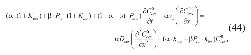
where x is the distance from the edge of the polymer wafer and ν_x is the x-component interstitial velocity. Combining the definition of α* in equation (23) and equation (26) for the apparent x-component of the velocity (analogous to the radial velocity), equation (27) for the apparent diffusivity, equation (28) for the apparent first-order elimination constant, and performing mathematical operations analogous to equations (22) to (36), equation (44) simplifies to

$$\frac{\partial C}{\partial t}+v_{app}\left(\frac{\partial C}{\partial x}\right)=D_{app}\left(\frac{{\partial }^{2}C}{\partial x^2}\right)-k_{app}C.$$

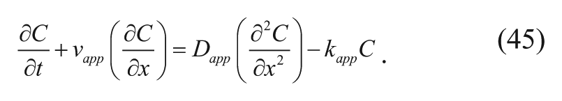
Assuming steady-state and negligible convection, equation (45) becomes

$$D_{app}\left(\frac{{\partial }^{2}C}{\partial x^2}\right)-k_{app}C=0.$$

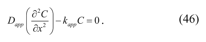
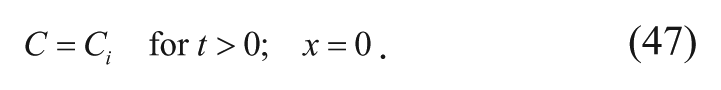
This differential equation is solved by applying two boundary conditions. First, at steady state, the concentration at the polymer-tissue interface (C_i) is assumed to be constant.

$$C=C_i\text{for}t>0;x=0.$$

Second, the flux at the edge of the brain is zero since empirically, the slope of the tangent of the concentration profile at the edge of the brain was measured to be zero ¹⁶ :

$$\frac{\partial C}{\partial x}=0\text{for}t>0;x=E,$$

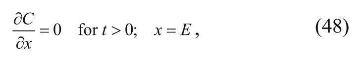
where the perpendicular distance from the edge of the polymer disk to the edge of the brain is defined as E. Applying the two boundary conditions above, the steady-state solution is ¹⁶

$$\frac{C}{C_i}=\frac{\exp \left(-\frac{E-x}{L}\varphi \right)+\exp \left(\frac{E-x}{L}\varphi \right)}{\exp \left(-\frac{E}{L}\varphi \right)+\exp \left(\frac{E}{L}\varphi \right)},$$

where L is half the thickness of the polymeric implant and the Thiele modulus is defined accordingly (see Appendix A for derivation):

$$\varphi =L\cdot \sqrt{\frac{k_{app}}{D_{app}}}.$$

Similar to the spherical coordinate case, there was little difference between the Thiele modulus predicted by the model and the Thiele modulus calculated with literature and estimated parameters. ¹⁶

Discussion on the Limitations of Simple Models

The solutions to the mathematical models were used to characterize drug transport in normal, nontumor brains of rats and monkeys and then compared with actual experimental data. This was done by using a cryostat to obtain 20-µm coronal sections of the animal brain and using quantitative autoradiography to quantify the concentration of ³H-labeled carmustine in the brain regions near the implant. Equation (39) in spherical coordinates and equation (49) in Cartesian coordinates were subsequently fit to the data for the rat brain and monkey brain, respectively. Local concentration profiles were used to yield a fitted value for the Thiele modulus. The good agreement between these values to that of the Thiele modulus calculated with other literature and approximated parameters demonstrated the validity of the simplified equations to describe the distribution of carmustine in animal brains.^15,16

However, it is necessary to understand that the analytical solutions derived for the 1D models are based on a few assumptions that may not hold true in all cases. For example, the equations are obtained by using boundary conditions such that the volume of the polymeric implant does not degrade over time. In reality, the Polifeprosan 20 pellet is biodegradable, which contributes to a receding boundary as a function of time.

Second, steady state is assumed. Accordingly, the concentration of drug at the polymer-tissue boundary is assumed to be constant. However, the concentration at the edge of the disk actually decreases with time.

In addition, ignoring fluid convection is not entirely appropriate since edema and fluid movement are characteristic symptoms in brain tumors after cranial surgery and may play a significant role in drug distribution shortly after. This is seen in the evaluation of carmustine’s effective penetration distance, which is defined as the distance at which the concentration is 10% of its peak value. The studies conducted in rat and monkey brains show that the penetration distance is substantially longer at early time points in the experiment in comparison to later times. This suggests that in addition to diffusion, enhanced interstitial fluid convection is a significant transport method as a consequence of postoperative cerebral edema.^15,16,22

Nevertheless, these three assumptions have not contributed any appreciable errors in the simplified models. First, it is reasonable to assume that the volume of the polymeric implant remains constant over the course of diffusion since the system delivers drug prior to any significant degradation. ¹⁷ The simplified models were also able to effectively characterize carmustine distribution over the majority of the disk’s initial drug delivery period.^15,16 Compared with the 6 to 8 weeks for the polymeric disk to completely degrade, ²³ the implant should experience little to no volume change during the estimated 30 days it takes for the polymer to deliver 90% of its payload.^15,16,24 Likewise, it is acceptable to assume that the concentration at the edge of the implant is constant. Over the time scale of interest (30 days), the concentration remains approximately constant. ¹⁵ The third assumption is reasonable as well since 3 days after implantation, enhanced bulk flow becomes negligible.^15,16,22 Accordingly, the simplified transport models neglecting convection are valid for the remaining days of the experiment.

In any case, these assumptions could be relaxed to improve the quantitative accuracy of the simplified 1D models. These neglected effects can be incorporated into the presented equations to more rigorously represent the sustained delivery of carmustine in the brain and can even be extended to 3D models. Evaluation of the significance of the various transport and elimination mechanisms would necessitate further research. Specifically, 3D models can capture another aspect of the system that cannot be quantitatively described in one dimension. Three-dimensional models are able to reconstruct the brain with asymmetrical geometry that captures the physical properties that vary depending on the different regions of the brain. Moreover, computer simulations can be used to predict the distribution of drug in a region and offer qualitative and quantitative data on the relative importance of processes like convection.

Three-Dimensional Computer Simulations of Carmustine Delivery

The previously discussed transport models describe 1D drug distribution in a simple geometry. In addition, most of the models assume bulk convection to be negligible compared with drug diffusion and drug elimination. In reality, the shape of the brain is asymmetric and drug is delivered in three dimensions. In the case of brain tumors, the elevated interstitial pressure in tumor tissue is known to cause considerable convective flux in the extracellular space, which may ultimately affect the distribution of drug uptake into cells.^{25 –27} A sophisticated theoretical model of drug transport in the brain should not only account for the anatomy of a real brain but also consider factors such as the effects of interstitial fluid flow that result from tumor-induced pressure gradients and transient postsurgical edema.

Use of the Finite Element Method

In recent years, research groups have started using computer simulations and a system of extended mathematical equations to predict drug distribution from a polymer implant in two and three dimensions. To address the issues of asymmetry, these simulations often incorporated the finite element method. This method divides a predetermined domain into simple shapes defined as finite elements. ²⁸ The differential equations of interest are then integrated over each element and the solutions at the boundaries of adjacent elements are matched to generate approximate solutions to the equations over the whole domain.

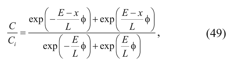
The finite element method (FEM) is especially applicable to modeling drug distribution in brain tumors since the irregular domain can be defined to be identical in size and shape to that of a realistic brain. With the use of MRI data, a 2D or 3D finite element mesh can be constructed to match the anatomical geometry of a rabbit or human brain ( Fig. 3 ). In addition, FEM has the advantage of including dissimilar material properties and capturing local effects. Important physical properties that are likely to influence drug distribution can be established at each point in the domain based on anatomical tissue sections. In 1995, Reisfeld et al. ²¹ used MRI data and FEM to model the 2D distribution and clearance of cisplatin, dexamethasone, and nerve growth factor delivered to the rabbit brain by intracranial implantation. Their model was later extended to incorporate the distinguished physical transport properties of white and gray matter of the brain, the boundary effect of ventricles, and the effect of edema on convective transport. ²⁸ Although their studies focused on a normal brain lacking any tumor, their general model has been used in further studies to simulate the transport of carmustine and other drugs in tumor tissue. ²⁹ The governing equations used in the carmustine models include the drug conservation equation as well as mass balance and linear momentum conservation equations that account for the convection of interstitial fluid. We will now describe the key equations of the models separately and describe how they are incorporated into the model.

Figure 3.

Example of a finite element geometry obtained from a patient with a brain tumor. The 3D reconstruction illustrates the ventricle (in blue), tumor (in red), and remaining brain tissue. Reprinted from Arifin et al. ²⁹ with permission from Elsevier.

Transport of Interstitial Fluid

The brain interstitium is assumed to be a rigid, porous medium. For this reason, the equations governing interstitial fluid transport have been described by coupling modified mass balance (or continuity) and momentum equations for fluid flow in a porous medium. We will first introduce the mass balance equation for a steady-state incompressible fluid, which describes the divergence of fluid velocity as equal to the combined rates of fluid gain and loss in a representative elementary volume. The mass continuity equation can be written as

$$\overrightarrow{\nabla }\cdot {\overrightarrow{v}}_{app}=F_V-F_l,$$

where ${\overrightarrow{v}}_{app}$ is the velocity of the interstitial fluid (and can have components in multiple directions), F_v is the rate of fluid gain from the blood per unit, and F_t is the rate of fluid removal from lymphatics per unit volume of tumor.^30,31 Wang and coworkers ³² argued that since the brain lacks a well-defined lymphatic system, the fluid removal term is neglected. The fluid gain term, which depends on the pressure difference between blood vessels and interstitial fluid, is described by Starling’s law ³⁰ :

$$F_V=K_V\left(\frac{S}{V}\right)\left[P_V-P_i-{\sigma }_p\left({\pi }_V-{\pi }_i\right)\right],$$

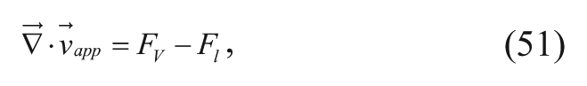
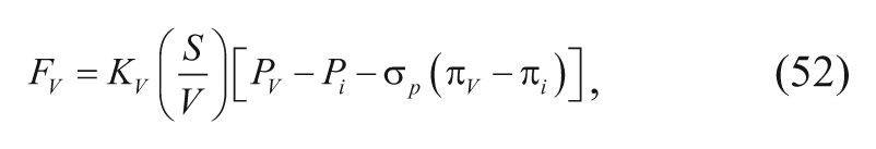
where K_v is the hydraulic conductivity of the microvascular wall, S/V is the available exchange area of the blood vessels per unit volume, P_v is the vascular pressure, P_i is the pressure of the interstitial fluid, σ_p is the osmotic reflection coefficient for plasma proteins, and π_v and π_i are osmotic pressures of blood plasma and interstitial fluid, respectively.

Conservation of Momentum and Darcy’s Law

The conservation of momentum, governed by the Navier-Stokes equations, can be simplified to Darcy’s law for low-velocity interstitial fluid flow through porous tissue^{33 –35}:

$${\overrightarrow{v}}_{app}=-\frac{\kappa }{\mu }\overrightarrow{\nabla }{P}_i,$$

where ${\overrightarrow{v}}_{app}$ is the bulk-volume average velocity, κ is the permeability of the porous interstitium, µ is the interstitial fluid viscosity, and $\overrightarrow{\nabla }{P}_i$ is the gradient of the bulk-volume average pressure (see Appendix B). Equation (53) is sometimes written as

$${\overrightarrow{v}}_{app}=-K\overrightarrow{\nabla }{P}_i,$$

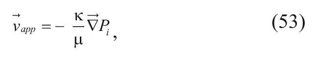
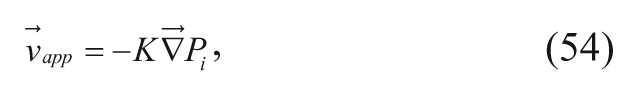
where the hydraulic conductivity, K, is equal to κ/µ.

The simplified Darcy’s law is shown to be sufficient in finite element simulations due to steady-state assumptions and the small value for the steady-state velocity of interstitial fluid through brain tissue (around 10⁻⁶ cm/s). ³² By substituting equation (54) into equation (51), a pressure field within the FEM domain can be calculated to describe the interstitial fluid velocity at any point. Coupling the pressure field with the drug conservation equation incorporates the convective influence in the mathematical prediction of drug distribution.

Drug Distribution in the Isolated Tumor Model

Drug distribution and modifications to the drug conservation equation largely depend on the physical boundaries that are represented in the model. One approach is the “isolated tumor model,” which focuses on drug distribution through uniform boundary conditions in the vicinity of the tumor. This model was used by Wang and coworkers, ³² who used MRI of a human primitive neuroectodermal tumor (PNET) to construct a 3D finite element mesh representing a human brain. In this simulation, the central 80% of tumor was removed from the model geometry and the polymer wafers were implanted in the resulting cavity. In contrast to the simulations by Kalyanasundaram and coworkers ²⁸ that use the anatomy of the rabbit brain, simulations performed using the anatomy of a human brain must account for the fact that the human brain tumor is relatively large (about 4 cm in diameter) compared with the penetration distance predicted for a single polymer implant. For this reason, the simulations focus on the drug distribution and concentration profiles through distinct zones of the tumor. Figure 4 shows the schematic of the surgical model that was used, in which each domain represents a different concentration profile depending on the density of tumor tissue and the presence of  blood vessels. The inner necrotic core of the tumor (domain B) refers to the tumor removed during surgical operation and hence is assumed to be devoid of blood capillaries. The tumor periphery, also denoted the viable zone (domain C), and the surrounding normal tissues (domain D) are shown to contain different amounts of blood vessels. N₁ to N₄ are the normal unit vectors corresponding to boundaries Ω₁ to Ω₄. Ω₁ is the polymer-tissue interface and Ω₄ is the external boundary of the brain. Each domain has a characteristic value of hydraulic conductivity, K, and diffusion coefficient, D, subscripted with the letter of its respective domain.

Figure 4.

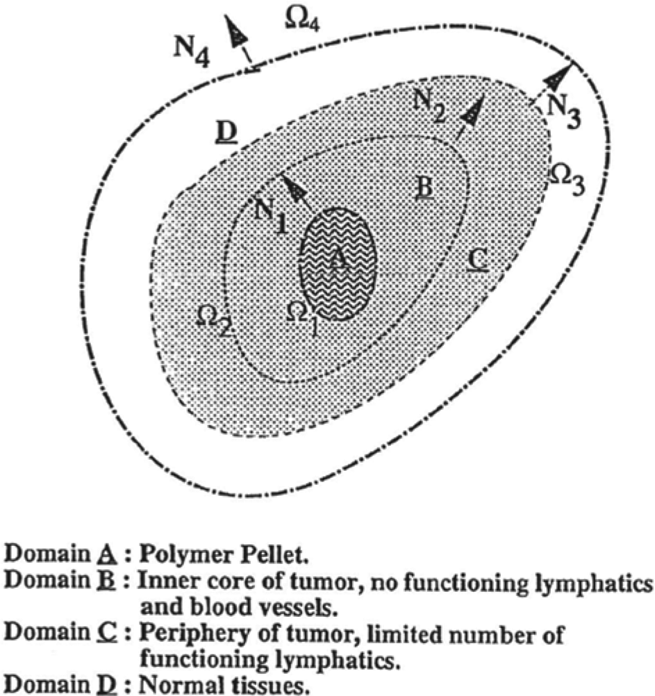
Schematic diagram of isolated tumor model. N₁ to N₄ are the normal unit vectors corresponding to boundaries Ω₁ to Ω₄. Reprinted from Wang et al. ³² with permission from Elsevier.

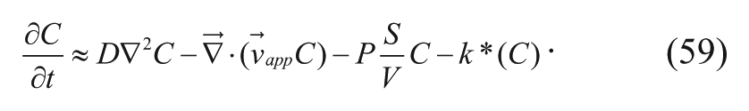
With regard to mass transport of the drug, Wang and coworkers ³² use the following drug concentration equation that applies for each domain:

$$\frac{\partial C}{\partial t}=D{\nabla }^{2}C-\overrightarrow{\nabla }\cdot ({\overrightarrow{v}}_{app}C)+F_S-F_{ls}-k*(C),$$

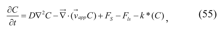
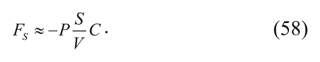
where C is the drug concentration, D is the drug diffusion coefficient in the interstitium, F_s is the supply of drug from the bloodstream per unit volume of tumor, F_ls is the loss of drug from the lymphatic vessel per unit volume of tumor, and k^* is a lumped first-order elimination rate constant that incorporates nonenzymatic reactions and Michaelis-Menten kinetics in the limit of low substrate concentration. Since there is no well-defined lymphatic system in the brain tissue, the F_ls term is assumed to be negligible. By referring to the work of Baxter and Jain, ³⁰ Wang and coworkers ³² defined the F_s term in the necrotic core, viable zone, and normal tissues as follows:

$$F_S=F_V(1-{\sigma }_d)C_V+P\frac{S}{V}(C_V-C)\left(\frac{P_{ev}}{e^{P_{ev}}-1}\right),$$

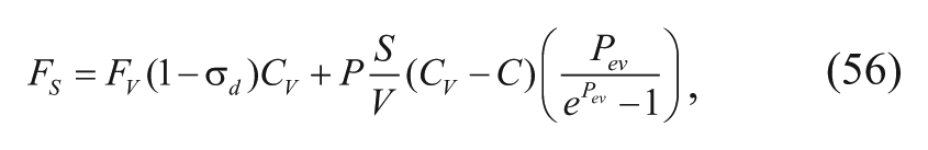
where σ _d is the osmotic reflection coefficient for the drug molecule, P is the vascular permeability coefficient, C_v is the concentration of drug in the plasma, and P_ev is the dimensionless transcapillary Péclet number as defined as follows ³¹ :

$$P_{ev}=\frac{F_V(1-{\sigma }_d)}{P(S/V)}.$$

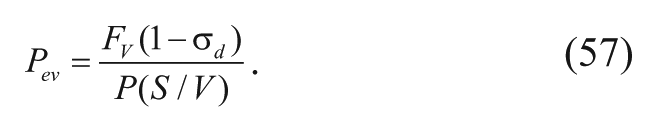
The concentration of initial drug in the plasma is assumed to be negligible, and thus $C_V\approx 0$ . Since carmustine has high transcapillary permeability, it has a small Péclet number (0.03–0.3 in neoplastic and normal tissue). ³² These values simplify equation (56) as follows:

$$F_S\approx -P\frac{S}{V}C.$$

Equation (58) can then be substituted into equation (55) to yield

$$\frac{\partial C}{\partial t}\approx D{\nabla }^{2}C-\overrightarrow{\nabla }\cdot ({\overrightarrow{v}}_{app}C)-P\frac{S}{V}C-k*(C).$$

The relevant boundary conditions for equation (59) include the equality of drug concentrations (where the partition coefficient is equal to 1) (equation (60)), interstitial fluid pressure (equation (61)), interstitial fluid flux (equation (62)), and molar flux of drug (equation (63)) and are shown below for the Ω₂boundary:

$${C|}_{{\Omega }_2^{-}}={C|}_{{\Omega }_2^{+}},$$

$${P_i|}_{{\Omega }_2^{-}}={P_i|}_{{\Omega }_2^{+}},$$

$${-K_{\underset{\_}{B}}\frac{\partial P_i}{\partial N_2}|}_{{\Omega }_2^{-}}={-K_{\underset{\_}{C}}\frac{\partial P_i}{\partial N_2}|}_{{\Omega }_2^{+}},$$

$${-D_{\underset{\_}{B}}\frac{\partial C}{\partial N_2}|}_{{\Omega }_2^{-}}+{({\overrightarrow{v}}_{app,N2}C)|}_{{\Omega }_2^{-}}={-D_{\underset{\_}{C}}\frac{\partial C}{\partial N_2}|}_{{\Omega }_2^{-}}+{({\overrightarrow{v}}_{app,N2}C)|}_{{\Omega }_2^{-}},$$

where ${\overrightarrow{v}}_{app,N2}$ is the component of ${\overrightarrow{v}}_{app}$ that is parallel to the direction of the respective unit vector N₂, D _B and D _C are the drug diffusion coefficients, and K _B and K _C are the hydraulic conductivities for domains B and C, respectively. Similar expressions are also applied to the Ω₃ boundary between domains C and D. There is assumed to be no outward flux at the Ω₄ boundary and no inward flux at the center of the polymer implant. At the polymer-tissue interface (Ω₁), the boundary condition of drug flux was matched in accordance with the in vivo data of carmustine delivery from ethylene-vinyl acetate copolymer by Yang and coworkers. ³⁶ Once the mathematical equations for fluid flow and drug distribution were established, values for the given variables were selected from previously published experimental data and entered in the computer simulations.^{20,30,31,36,37} Results from simulations of polymer implanted in the necrotic core and viable zone proved little difference in drug distribution compared with the results in which the interstitial and transcapillary convection terms in equation (55) were ignored. This indicates that the diffusion and pseudo–first-order elimination terms dominate the drug distribution in the necrotic core and viable regions of the tumor. Although there was little difference between the results, the difference was due to the small transcapillary Péclet number for carmustine, which suggests that a smaller transcapillary permeability (which would lead to a greater transcapillary Péclet number) could lead to greater differences in simulation results.

Drug Distribution in a Full Brain Model

In a more recent study, Teo and coworkers ²⁶ stated that the isolated tumor model has a disadvantage, since certain boundary conditions will vary depending on the tumor location. More specifically, the pressure boundary conditions will not be accurate depending on where the isolated tumor model is located. Instead, they used a model that captures drug distribution in the entire brain by dividing the brain tissue into three phases, similar to the models of Fung and coworkers ¹⁵ and Saltzman and Radomsky. ²⁰ Two physiologically accurate boundaries were defined: the innermost boundary is the surface of the ventricle and the outermost boundary is the arachnoid villi on the outermost surface of the brain. ² The assumptions made in the 1D models for the drug behavior and distribution of carmustine are valid in this case as well. The model geometry used in this study was constructed from magnetic resonance images of a patient with glioblastoma. Most of the tumor was removed from the geometry to form a cavity in which eight Gliadel wafers with a total carmustine dosage of 61.6 mg were placed, with surrounding residual tumor.

Using the expressions for average concentrations in equations (6) and (7), equation (11) can be applied to the 3D model. All drug within the cavity is considered to be in the interstitial/ECS phase and able to be transported. When the drug conservation equation is coupled with flow equations, drug transport in the cavity is described as follows:

$$\frac{\partial C_{ecs}^0}{\partial t}=D_{ecs}{\nabla }^2{C}_{ecs}^0-{\overrightarrow{v}}_{app}\cdot \overrightarrow{\nabla }{C}_{ecs}^0-k_{ecs}{C}_{ecs}^0,$$

where k_ecs is the first-order degradation constant in the cavity. Note that this is the general form of equation (29) and that the convection term is described by the flow equations, equations (51) and (54). Boundary conditions for the simulation studies include the continuity of drug flux across all internal boundaries. At the ventricle and outer brain boundaries, the concentrations of drug were set to zero, and pressures were set at constant values of 1447.4 Pa and 657.9 Pa, respectively. ³⁸

Discussion on the Advantages of Computer Simulations

In recent years, the shift toward computer simulations has helped elucidate important factors that affect the distribution of carmustine. One prevalent factor is the effect of transient edema after surgical resection, which results in fluid accumulation and relatively high pressures in the cavity and surrounding remnant tumor. This effect over the first days of implantation in vivo could not be explained by simplified 1D models but has been modeled in greater detail with simulations. In the full-brain simulation, Arifin and coworkers ² captured the effect of edema by introducing a time-dependent change in the hydraulic conductivity of the remnant tumor, which increases and then resolves in a 3-day time span. The results of these simulations suggest that increased interstitial fluid production in the cavity produces a convection of fluid away from the polymer implant toward outer boundaries of the brain, consequently contributing to the large spread of carmustine over the first 24 h after implantation. The spread is soon reduced as edema resolves over the next 48 h. However, carmustine is shown to exist at the remnant tumor in therapeutic concentrations (above 15 µM) for only about 5 days and only in the immediately adjacent tissue (less than 2 mm from the implant). This is most likely due to another important factor: the high transcapillary permeability lends carmustine to rapid elimination through the capillaries. Future studies seeking to optimize the Gliadel wafer system should consider fluid convection as well as the properties of the drug itself. The same computer simulations can also be used to model and compare the distribution of various cancer chemotherapeutics with that of carmustine. ²⁹

The effect of polymer degradation on drug release is still an issue that has yet to be explored. There remains no well-defined model of drug release from a biodegradable polymer such as Polifeprosan 20. Most studies assume an ideal zero-order process in which the initial drug dosage is released at a constant rate for a period of weeks. In reality, drug release from Gliadel wafers does not remain constant as the release mechanism is influenced by the time-dependent hydrolysis of the chemical linkages of the polymer and subsequent degradation. This assumption was relaxed in the full-brain simulation by Arifin and coworkers ² by matching drug release to the in vivo release profiles in normal rat brains, which described an initial burst of about 70% of the total loading during the first 24 h, followed by a more constant release rate in the following hours. This drug release model can be modified to account for polymer degradation in the interstitial environment of the human brain in the future.

In conclusion, implantable drug delivery systems provide a viable solution to overcome the problems and difficulties presented with the systemic delivery of chemotherapeutics. Surgical implantation of biocompatible controlled-release devices directly onto the target site requires only modest drug amounts to achieve high local concentrations for extended periods, limiting the necessity to deliver large drug dosages throughout long distances in the body. Carmustine wafers are useful for the treatment of recurrent malignant glioma after surgical removal of the tumor, as the interstitial delivery of carmustine bypasses the BBB and penetrates adjacent tissue without exposing other portions of the brain to cytotoxic concentrations. Mathematical models have been able to accurately characterize the distribution of carmustine following implantation, a feat otherwise impossible to predict in humans without invasive operations. The results have shown that carmustine is transported primarily via diffusion, although promptly after surgery, the delivery is also affected by the convection of extracellular fluid caused by vasogenic edema, which resolves after the third day. Furthermore, it is seen that carmustine’s penetration distance is limited by its lipophilicity, and carmustine is prone to rapid elimination from the body due to its high transvascular permeability. This knowledge can help improve the efficacy of future drug delivery implants.

Mathematical models can be used to describe drug release and transport in the brain. Such modeling has proved instrumental in developing a better understanding of the system. The usefulness of this approach can be modified to apply to other systems using a similar theoretical framework. Quantitative analyses provided by governing equations and computer simulations can give insight to trends and behaviors of a system that can help save time and resources in experimentation.