Mathematical Modeling of Vesicle Drug Delivery Systems 2

Abstract

Vesicles have been studied for several years in their ability to deliver drugs. Mathematical models have much potential in reducing time and resources required to engineer optimal vesicles, and this review article summarizes these models that aid in understanding the ability of targeted vesicles to bind and internalize into cancer cells, diffuse into tumors, and distribute in the body. With regard to binding and internalization, radiolabeling and surface plasmon resonance experiments can be performed to determine optimal vesicle size and the number and type of ligands conjugated. Binding and internalization properties are also inputs into a mathematical model of vesicle diffusion into tumor spheroids, which highlights the importance of the vesicle diffusion coefficient and the binding affinity of the targeting ligand. Biodistribution of vesicles in the body, along with their half-life, can be predicted with compartmental models for pharmacokinetics that include the effect of targeting ligands, and these predictions can be used in conjunction with in vivo models to aid in the design of drug carriers. Mathematical models can prove to be very useful in drug carrier design, and our hope is that this review will encourage more investigators to combine modeling with quantitative experimentation in the field of vesicle-based drug delivery.

Overview

Drug delivery involving the use of vesicles as drug carriers has been successful both in vitro and in vivo. Within the classification of vesicles, these nanoscale materials can be referred to as liposomes, when they are composed of lipids, or polymersomes, when they are composed of polymers.^1,2 In addition, polymersomes composed of polypeptides have been referred to as polypeptide vesicles. ³ All of these vesicle-based drug delivery vehicles have several advantages, such as protecting the drug from degradation, increasing drug half-life in the blood, targeted delivery of chemotherapeutics to cancer cells, and controlled release of the encapsulated therapeutics.

Mathematical modeling can be combined with quantitative experiments to reduce the time and resources required to optimize vesicle-based drug delivery systems. This article is the second of two review papers that summarize equations that can be used to engineer these drug carriers. Together, the two articles consider molecular to whole-body length scales in identifying approaches to optimize these vesicles. The first article focused on molecular and vesicular length scales, as models for vesicle formation and stability, as well as drug loading and release, were discussed. This follow-up review article considers cell, tumor, and whole-body length scales. Specifically, it analyzes vesicles binding to and being internalized by cancer cells, the competing factors involved as vesicles diffuse into tumors, and the distribution and clearance of vesicles from the body. The goal of our review is to encourage more researchers in this exciting field of vesicle-based drug delivery to combine mathematical models with experimentation for designing these drug carriers.

Targeting and Uptake

Introduction

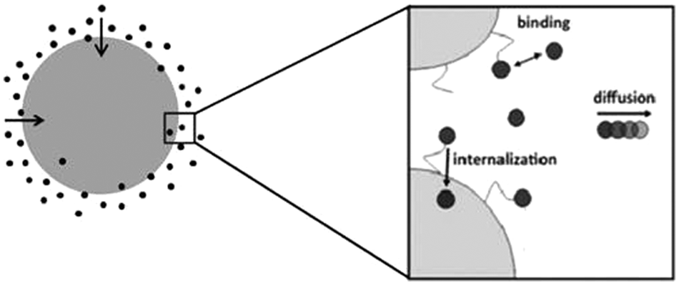
Vesicles can selectively accumulate in tumor tissue via the enhanced permeability and retention (EPR) effect. This phenomenon results from the tumor tissue’s leaky vasculature, which allows particles between 60 and 400 nm to enter the tumor tissue more easily, and poor lymphatic drainage, which reduces the clearance of these particles from the tissue. To improve vesicle uptake into cancer cells once they are in the tumor region, researchers have been conjugating targeting ligands to the vesicle surface. Due to their highly proliferative nature, many cancer cells overexpress surface receptors for proteins that facilitate their rapid growth, such as the iron-carrier protein transferrin. Vesicles conjugated to targeting ligands can then specifically bind to cell-surface receptors instead of adsorbing nonspecifically to the cell surface. They can then be internalized into cells via the ligand’s intracellular trafficking pathway. Because multiple ligands can be conjugated to a single vesicle, the vesicles can also benefit from a multivalency effect that can enhance their binding affinity for the cell-surface receptors. If one ligand dissociates from its receptor, other existing ligand-receptor interactions can aid in holding the vesicle in place.

Vesicles can enter cells via receptor-mediated endocytosis by first binding to the cell-surface receptors. A vesicle’s specific binding to the cell surface occurs when ligand-receptor interactions form between the vesicle and the cell surface. However, these interactions are not permanent, and ligands can unbind from their receptors. In this review, we will focus on situations where the cell surface expresses the receptors and the ligands are conjugated to the vesicles.

Mathematical models derived using mass-action kinetics have been used to examine cellular uptake of various macromolecules and particles with diameters less than 200 nm.^4–6 Since vesicles fall within this size range, the models can also be used to evaluate vesicle uptake. Most models take a simplified approach by treating the vesicle-to-binding site interaction as 1:1. For a single ligand-receptor interaction, the receptor is considered as one binding site. For a vesicle-receptor interaction, since multiple ligand-receptor interactions can form, the cluster of interacting receptors can be assumed to represent one binding site. This approach will be discussed first, followed by a model that accounts for the vesicle’s multivalency effect.

The primary purpose of these models is to quantitatively evaluate the rate at which vesicles containing drugs are able to enter cells. To achieve maximal cellular uptake of vesicles, the vesicle should exhibit high-affinity binding to the cell surface and a high rate of internalization into the cell. The following sections will examine how various experimental procedures can be used in conjunction with the mathematical models to determine the rate constants that characterize the uptake process of vesicles.

The General Kinetic Model

The following model is represented by Figure 1 . Assuming that vesicle association to the cell surface is independent of other ongoing processes, the event can be described as

$$L+R_s\underset{k_d}{\overset{k_a}{\rightleftharpoons }}{C}_s,$$

where L is the free vesicle (with concentration units of molarity, M), R is the number of free binding sites (with concentration units of #/cell), C _s is the number of vesicles bound to the cell surface (with concentration units of #/cell), k _a (M⁻¹·s⁻¹) is the association rate constant for a free vesicle binding to a free binding site, and k _d (s⁻¹) is the dissociation rate constant for a vesicle dissociating from its binding site.

Figure 1.

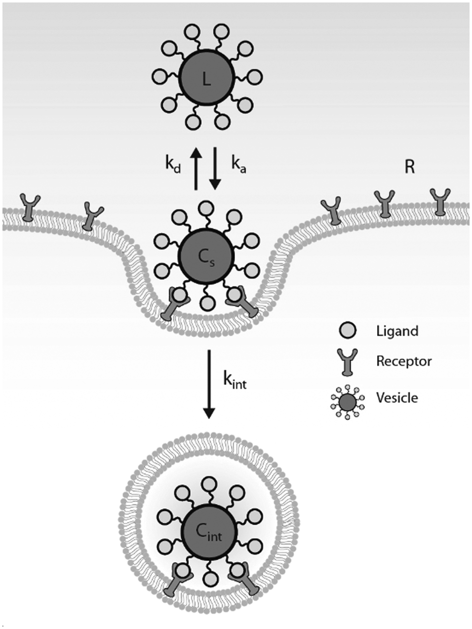
Illustration of the general kinetic model.

Upon associating to a free binding site, vesicles can be internalized into the cell via endocytosis. The internalization process can be described as

$$C_s\stackrel{k_{int}}{\to }{C}_{int},$$

where C _int is the internalized vesicles (with concentration units of #/cell), and k _int (s⁻¹) is the rate constant for a bound vesicle to be internalized. A species balance on the number of bound vesicles yields the following equation:

$$\frac{d{C}_s}{dt}=k_{a}L{R}_s-(k_d+k_{\mathrm{int}})C_s.$$

Regardless of the physical nature of the binding site, typical mathematical models generally assume that the number of binding sites remains constant over time, as the cell is constantly regenerating and internalizing its membrane. A species balance on the total number of binding sites, R _T , can therefore be expressed as follows:

$$R_T=R_s+C_s.$$

Association and Dissociation—Radiolabeling

We will first examine how radiolabeling techniques can be used to empirically determine the vesicle’s association and dissociation rate constants. In the literature, radiolabeling techniques have seldom been used in conjunction with mathematical modeling of the vesicle’s binding and dissociation properties. However, various research groups have used the combination of radiolabeling and modeling to evaluate the rate constants for transferrin’s (Tf) intracellular trafficking pathway. ⁷ The interaction between Tf and the Tf receptor (TfR) was treated as 1:1. Because this is in accordance with how most models treat the interactions between vesicles and their binding sites, the radiolabeling techniques that analyzed the Tf-TfR trafficking pathway can also be used to evaluate the rate constants for a vesicle’s trafficking pathway. In this case, the vesicle is analogous to the Tf protein, and the vesicle’s binding site is analogous to TfR.

In radiolabeling experiments performed by Ciechanover and coworkers, ⁸ Tf was radiolabeled with ¹²⁵I and allowed to bind to cell-surface TfR in a monolayer cell culture environment. Excess radiolabeled Tf and energy inhibitors were used to prevent generation of free receptors and receptor internalization, respectively. In addition, it was assumed that Tf does not dissociate significantly from TfR during the time course of the experiment, since excess radiolabeled Tf was used. Under these conditions, k _d and k _int can be neglected, and equation (3) was simplified to

$$\frac{d{C}_s}{dt}=k_{a}L{R}_s.$$

Equation (5) can be rewritten to only have R _s as a variable by solving for C _s in equation (4) and substituting into equation (5):

$$\frac{d{R}_s}{dt}=-k_{a}L{R}_s.$$

In this case, L represents the concentration of free Tf (M), R _s represents the number of free Tf receptors (#/cell), and C _s represents the number of Tf-TfR complexes on the cell surface (#/cell). L was assumed to remain constant over the time course of the experiment, since the Tf concentration in the medium was in excess in the experiment and was not expected to change significantly throughout the experiment. Equation (6) was then integrated and solved for R _s as a function of time. Upon applying the initial condition that the number of free receptors present on the cell surface at t = 0 is equal to R _T , the following equation was obtained:

$$\ln \left(\frac{R_s}{R_T}\right)=-k_{a}Lt.$$

The half-time (t = t_1/2) of association, or the time required for half the cell-surface receptors to be occupied, was determined by setting R _s to equal R _T /2 at t_1/2:

$$t_{1/2}=\frac{\ln (2)}{k_{a}L}.$$

The fraction of free receptors can also be expressed with the following equation:

$$\frac{R_s}{R_T}=1-\frac{C_s}{C_{\max }},$$

where C_max, or the maximum number of ligands that can bind to the cell surface, equals R _T if it is assumed that all receptors are occupied due to the addition of excess Tf. The number of cell-surface Tf-TfR complexes was determined by measuring the cell-associated radioactivity. Equation (9) was then used to determine the number of free cell-surface receptors. The half-time t_1/2 was determined by creating a semi-logarithmic plot of the fraction of free receptors (R _s /R _T ) as a function of time. With t_1/2 determined, equation (8) was used to evaluate the value of k _a .

Ciechanover and coworkers ⁸ also determined the dissociation rate constant for the Tf-TfR system by finding the half-time for dissociation. Similarly, radiolabeled Tf was allowed to bind to cells at 4 °C in the presence of energy inhibitors. The low temperature was also used to inhibit ligand internalization into the cell. After equilibrium was attained, unbound Tf was washed off, and excess unlabeled Tf was added to the medium. In the presence of excess unlabeled Tf, when radiolabeled Tf dissociates from its receptor, an unlabeled Tf will bind to the receptor. In addition, since excess unlabeled Tf is present, any dissociated radiolabeled Tf is assumed to not rebind to the receptor. Under these conditions, k _a and k _int can be neglected, and equation (3) was simplified to

$$\frac{d{C}_s}{dt}=-k_d{C}_s.$$

Similar to equation (6), equation (10) was solved for C _s as a function of time. Upon applying the initial condition that the number of cell-surface Tf-TfR complexes at t = 0 is C_s,0, and by setting C _s to equal C_s,0/2 at the half-time for dissociation (t_1/2, the time it takes for half the complexes to dissociate from the cell surface), t_1/2 was determined:

$$t_{1/2}=\frac{\ln (2)}{k_d}.$$

The half-time for dissociation was determined by creating a semi-logarithmic plot of the fraction of remaining cell-surface complexes (C _s /C_s,0) as a function of time. Equation (11) was then used to evaluate the value of k _d .

Surface Plasmon Resonance to Evaluate Multivalency—Method I

Surface plasmon resonance (SPR) has been used extensively to quantify the binding parameters between a ligand and its receptor, whether the ligand is by itself or is conjugated to a construct such as a vesicle. In these experiments, buffer containing the vesicle is injected across receptors immobilized onto a biosensor surface. Ligand-receptor interactions change the refractive index of the biosensor surface, and therefore, vesicle buildup on the biosensor surface can be detected as an increase in the refractive index. To individually determine k _a and k _d , the binding and dissociation experiments can be performed separately. Data from the SPR experiments can then be analyzed using biosensor kinetic data analysis programs such as CLAMP. This program generates various differential equations from the SPR data and a chosen binding model, where the model defines the number of interactions between the vesicle and the receptors. ⁹

The rate constants k _a and k _d can be related to the equilibrium dissociation constant, K _D , as defined in the following equation:

$$K_D=\frac{k_d}{k_a}.$$

From this equation, we can see that vesicles with smaller K _D values will have higher binding affinities for their receptors. Since the precise number of ligand-receptor interactions between a vesicle and the receptors is not easily discernable, Mammen and coworkers ¹⁰ defined an enhancement factor β that generally characterizes the binding affinity of multivalent constructs. β is represented by the following equation:

$$\beta =\frac{K_D^{free}}{K_D^{multivalent}},$$

where $$K_D^{free}$$ is the K _D of the targeting ligand alone, and $$K_D^{multivalent}$$ is the K _D of the multivalent construct. The value of $$K_D^{multivalent}$$ incorporates the potentially enhanced binding affinity of the construct from the effects of multivalency. As β increases, $$K_D^{multivalent}$$ decreases in magnitude compared to $$K_D^{free}$$ , indicating an increase in the binding affinity of the multivalent particle compared with that of the ligand itself.

Tassa and coworkers ¹¹ performed SPR binding experiments to determine the K _D values of their small molecule-modified, multivalent nanoparticles. They first quantified the $$K_D^{free}$$ of their targeting ligand by injecting a solution containing only ligand across receptors immobilized to a biosensor surface. Subsequently, they quantified the $$K_D^{multivalent}$$ of their nanoparticles by injecting a solution containing the ligand-conjugated particles across the same biosensor surface. They repeated this step multiple times, each time varying the ligand valency of their nanoparticles. Finally, they compared the values of β among their nanoparticles. Similar experimental methods, when combined with equations (12) and (13), can be used to compare the K _D values of vesicles of varying ligand valencies. Analysis of the binding affinity results can help optimize delivery of the vesicle as a drug carrier by optimizing the number of ligands conjugated per vesicle, as well as the identity of the ligand used.

The Multivalent Kinetic Model

To account for higher-order interactions between vesicles and cell-surface receptors, we can expand on the general kinetic model, as described by equation (3). Thus, we will no longer treat each binding site as a cluster of receptors since each individual receptor will be accounted for in the model. Similar to the general kinetic model, the total number of receptors is assumed to remain constant over time. Furthermore, each receptor is assumed to bind to only one ligand. The following equations were adapted from mathematical models that were used to analyze divalent and trivalent ligand constructs.^12,13 This model, shown in Figure 2 , will examine the first two ligand-receptor interactions between a vesicle and the cell surface.

Figure 2.

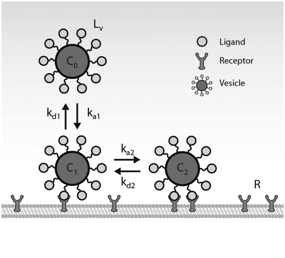
Illustration of the multivalent kinetic model.

The initial association of the vesicle with the cell surface can be described as

$$C_0+R_s\underset{k_{d1}}{\overset{k_{a1}}{\rightleftharpoons }}{C}_1,$$

where C₀ represents the vesicles with no ligands bound to the cell-surface receptors (M), R_s is the number of free cell-surface receptors (#/cell), and C₁ is the number of vesicles with one ligand bound to a cell-surface receptor (#/cell). The rate constants k_a1 and k_d1 represent the association and dissociation rate constants, respectively, for the first ligand-receptor interaction. A species balance on the number of cell-surface vesicles with no ligand bound yields the following equation:

$$\frac{d{C}_0}{dt}=-L_v{k}_{a1}{C}_0{R}_s+k_{d1}{C}_1,$$

where L _v is the number of ligands conjugated per vesicle. This factor accounts for the possibility that any ligand on the vesicle surface can associate with the cell-surface receptor. The next ligand-receptor association can be described as

$$C_1+R_s\underset{k_{d2}}{\overset{k_{a2}}{\rightleftharpoons }}{C}_2,$$

where C₂ is the number of vesicles with two ligands bound to two cell-surface receptors (#/cell). The rate constants k_a2 and k_d2 represent the association and dissociation rate constants, respectively, for the second ligand-receptor interaction. A species balance on the number of cell-surface vesicles with one ligand bound yields the following equation:

$$\frac{d{C}_1}{dt}=L_v{k}_{a1}{C}_0{R}_s-k_{d1}{C}_1-\left(L_v-1\right)k_{a2}{C}_1{R}_s+2k_{d2}{C}_2.$$

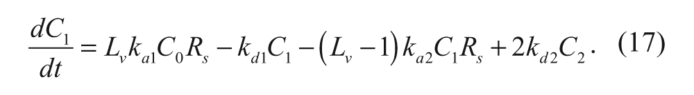
The factor of 2 in front of k_d2C₂ accounts for the possibility that either of the two ligands on the vesicle can dissociate with its receptor.

It should be noted that due to geometric limitations, not every ligand is accessible to a receptor once the vesicle has formed a ligand-receptor interaction with the cell surface. Thus, the factor in front of k_a2C₁R should be much less than (L _v – 1). Ghaghada and coworkers ¹⁴ have taken into account this limitation by geometrically determining the fractional area on their liposome that is available to interact with the cell surface. Furthermore, the ligands are often attached to the particle surface via flexible tethers such as polyethylene glycol, which not only provide in vivo stability to the particle but also allow the ligands to reach a greater cell-surface area and potentially access a greater number of cell-surface receptors. Thus, factors such as vesicle size, ligand and receptor densities on their respective surfaces, and the tether length ¹⁵ can affect the vesicle’s overall binding affinity.

SPR to Account for Multivalency—Method II

As previously described, Tassa and coworkers ¹¹ first fit their data to a 1:1 interaction model for their small molecule-modified nanoparticles. To account for the contributions to binding affinity by higher-order interactions, they reanalyzed their data by fitting them to a 2:2 interaction model, which corresponds to a bivalent interaction between the nanoparticle and the receptors. Because this model neglects the actual degree of nanoparticle multivalency, L _v is equal to 2, and equations (15) and (17) can be rewritten as

$$\frac{d{C}_0}{dt}=-2k_{a1}{C}_0{R}_s+k_{d1}{C}_1.$$

$$\frac{d{C}_1}{dt}=2k_{a1}{C}_0{R}_s-k_{d1}{C}_1-k_{a2}{C}_1{R}_s+2k_{d2}{C}_2.$$

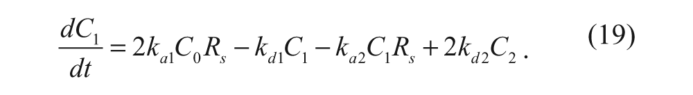
A species balance on the number of nanoparticles with two ligands bound can also be written as follows

$$\frac{d{C}_2}{dt}=k_{a2}{C}_1{R}_s-2k_{d2}{C}_2.$$

The model was not intended to realistically model the nanoparticle system as a whole. Rather, it was used as a means of estimating the contribution of higher-order interactions to the nanoparticle’s overall binding affinity. Since two sets of association and dissociation rate constants were obtained from the model, they found the K _D values for each ligand-receptor interaction as shown by the following equations:

$$K_{D1}=\frac{k_{d1}}{k_{a1}},$$

$$K_{D2}=\frac{k_{d2}}{k_{a2}}.$$

A comparison between the values of K_D2 and K_D1 can potentially provide some insight into the nature of multivalent interactions. If the value of K_D2 is less than K_D1, this indicates that the second interaction displays a higher binding affinity than the first interaction. The increase in the second interaction’s binding affinity has the potential to increase the overall binding affinity of the particle to the cell-surface receptors.

Internalization

We will now examine two radiolabeling methods that can empirically determine the internalization rate constant of Tf once it has bound to a cell-surface TfR. As mentioned previously, these radiolabeling techniques can be adapted to determine a vesicle’s internalization rate constant as well, since a 1:1 interaction can be used to mathematically model Tf-TfR interactions and to approximate multivalent vesicle-receptor interactions.

In the first method, Ciechanover and coworkers ⁸ allowed radiolabeled Tf to bind to cells at 4 °C to achieve maximum binding. After unbound Tf was washed off, excess unlabeled Tf was added to the medium at physiological temperature. The excess unlabeled Tf prevents rebinding of dissociated radiolabeled Tf, and the temperature increase helps to facilitate the endocytosis process. Under these experimental conditions, equation (3) was rewritten as

$$\frac{d{C}_s}{dt}=-\left(k_d+k_{\mathrm{int}}\right)C_s.$$

Equation (23) was rearranged and integrated to solve for C _s as a function of time. Upon applying the initial condition, where the number of Tf-TfR complexes on the cell surface at t = 0 is C_s,0, and by setting C _s to equal C_s,0/2, t_1/2 for internalization was obtained:

$$t_{1/2}=\frac{\ln (2)}{k_d+k_{\mathrm{int}}}.$$

The value of k _d was obtained from the results of the radiolabeling experiments as discussed earlier. The half-time of internalization was determined by making a semi-logarithmic plot of the fraction of remaining cell-surface complexes (C _s /C_s,0) as a function of time. Equation (24) was then used to determine the internalization rate constant.

In the second method, the In/Sur plot, as described by Wiley and Cunningham, ¹⁶ was used to evaluate the internalization rate constant of the Tf-TfR complex. A species balance on the number of internalized Tf-TfR complexes yields the following equation:

$$\frac{d{C}_{int}}{dt}=k_{int}{C}_s+\left(k_{deg}-k_{rec}\right)C_{int},$$

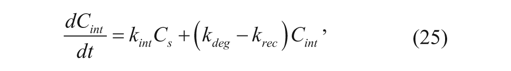
where k _deg is the degradation rate constant of the internalized complex (s⁻¹), and k _rec is the recycling rate constant of the internalized complex (s⁻¹). Using short time periods (under 6 min), where linear accumulation of internalized complexes was observed, k _deg and k _rec can both be neglected since the Tf must be internalized before it can be degraded or recycled. Equation (25) becomes

$$\frac{d{C}_{int}}{dt}=k_{int}{C}_s.$$

Assuming that the number of cell-surface complexes does not change significantly over the time course of the experiment, equation (26) can be integrated to solve for C _int as a function of time. By applying the initial condition that no complexes are inside the cell at t = 0, equation (26) becomes

$$C_{int}=C_s{k}_{int}t.$$

Gironès and Davis ¹⁷ used the In/Sur plot along with their own experimental procedure to determine the internalization rate constant of the Tf-TfR complex. Cells were incubated with radiolabeled Tf for a short time period, and the total radioactivity was measured. An acid wash removed surface-bound complexes, and the remaining cell-associated radioactivity was measured. Finally, the number of surface-bound complexes was found by subtracting the cell-associated radioactivity from the total radioactivity. The ratio of internalized complexes to surface-bound complexes, C _int /C _s , was plotted versus time, and k _int was found from the slope.

Alternatively, if the number of surface-bound complexes is not assumed to be constant over time, equation (27) can be rewritten as

$$C_{int}=k_{int}{\displaystyle {\int }_0^T{C}_s(t)dt},$$

where T is the time period of the experiment. The integral of the number of surface-bound complexes over the time period of interest can be estimated by the trapezoidal and Simpson’s rules. For both equations (27) and (28), the ratio of internalized complexes to surface-bound complexes can be plotted versus time, and k _int can be then determined by calculating the slope of the plot.

Intratumoral Diffusion

Introduction

In the early stages of investigating the therapeutic efficacy of vesicles as drug carriers, studies are often conducted with in vitro monolayer cell cultures. However, verified in vitro design criteria may not apply to in vivo situations due to the geometric difference between a monolayer cell culture and a tumor tissue. Therefore, spheroids have been used to better mimic the geometry of tumor tissues. In the case of tumor spheroids, the vesicles’ binding affinity to cell-surface receptors and their subsequent internalization into tumor cells are not the only factors governing their therapeutic efficacy. Deeper penetration into the tumor core, leading to a more homogeneous vesicle distribution throughout the tumor, is also desired for an enhanced therapeutic effect. Various groups have observed penetration of particles into both spheroids and tumor tissue. Waite and Roth ¹⁸ observed the delivery of targeted dendrimer/siRNA complexes with a diameter of 190 nm throughout a 100-µm spheroid. These particles range from 100 to 200 nm, which is also a common size range for vesicles. Kirpotin and coworkers ¹⁹ also reported the distribution of liposomes with diameters of 90 to 110 nm in xenograft tumor tissue. Accordingly, researchers in the vesicle field can take advantage of mathematical models that have been developed to better understand the penetration process, including diffusion, binding, and internalization of drug carriers. This understanding can then be used to help guide experimental strategies to improve drug distribution and thus efficacy.

Basic Model

Several research groups have developed mathematical models to describe diffusion, binding, and internalization of drugs in tumor spheroids ( Fig. 3 ). Parameters included in the model can potentially be engineered to maximize the penetration of drugs into tumor spheroids. The drugs of interest used in previous models range from several nanometers (such as an antibody) up to 200 nm (such as a viral vector), but they share a similar mathematical model.^20–22 Most models consider tumor spheroids as strictly spherical and assume no convection inside the spheroid.

Figure 3.

The three main processes considered are as follows: (a) association and dissociation of vesicles, (b) internalization of bound vesicles, and (c) diffusion of free vesicles. Reprinted by permission from the American Association for Cancer Research: Mok, W., Stylianopoulos, T., Boucher, Y., R. K. Jain, Mathematical modeling of herpes simplex virus distribution in solid tumors: implications for cancer gene therapy, Clinical Cancer Research, 2009, 15:7, 2352-2360.

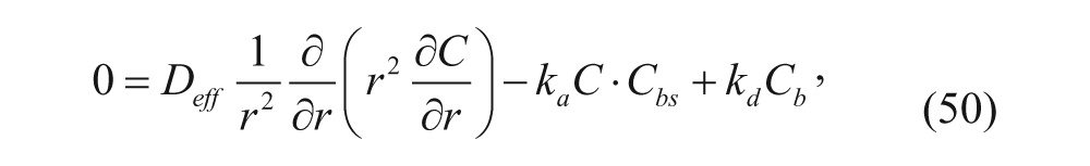
A general mathematical model for diffusion of vesicles can be written based on the conservation of species equation. ²⁰ Parameters such as diffusion, association, and dissociation between vesicles and binding sites on the cell membrane all govern the concentration profile of free vesicles in the spheroid, as shown in equation (29):

$$\frac{\partial C}{\partial t}=\frac{1}{r^2}\frac{\partial }{\partial r}\left[D_{ef{f}_{(r)}}{r}^2\frac{\partial C}{\partial r}\right]-k_2{C}_{bs}C+k_d{C}_b,$$

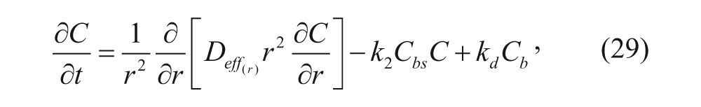
where C is the concentration of free vesicles per tumor volume (M), r is the radial coordinate (m), t is time (s), k _a is the association rate constant (M⁻¹·s⁻¹), k _d is the dissociation rate constant (s⁻¹), and D _eff is the effective diffusion coefficient (m²·s⁻¹). At the center of the spheroid, r = 0, whereas at its outer rim, r = R. In most cases, D _eff is assumed to be a constant throughout the spheroid. However, Goodman and coworkers ²³ obtained D _eff as a function of r considering the structural difference between the outer proliferating rim, the middle quiescent region, and the necrotic core region. The measurement of the effective diffusion coefficient will be discussed later.

Similarly, the concentrations of the bound vesicles, the available binding sites on cell surfaces, and the internalized vesicles can be represented as follows, where association and dissociation between vesicles and cell membranes, the internalization of vesicles, and the regeneration of binding sites are considered:

$$\frac{d{C}_b}{dt}=k_a{C}_{bs}C-k_d{C}_b-k_{int}{C}_b,$$

$$\frac{d{C}_{bs}}{dt}=-k_a{C}_{bs}C+k_d{C}_b+R_s,$$

$$\frac{d{C}_i}{dt}=k_{int}{C}_b,$$

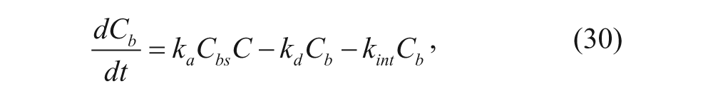
where C _bs , C _b , and C _i are concentrations of unbound binding sites, bound vesicles, and internalized vesicles per tumor volume (M), respectively, and k _int is the internalization rate constant (s⁻¹). R _s is the synthesis rate of new binding sites (M·s⁻¹). Most models assume that the number of regenerated binding sites is equal to the number of internalized bound vesicles, represented by k _int C _b .

Since the spheroid is considered a perfect sphere and the concentration of free vesicles is independent of θ and ϕ, the flux at the center is equal to 0 by spherical symmetry, as described by the following boundary condition:

$$\frac{\partial }{\partial r}\left[C_{(t,r=0)}\right]=0.$$

Another boundary condition is r = R, where the concentration of free vesicles remains constant and equals ϵC₀, where ϵ is the partition coefficient between the spheroid and the external solution. Note that ϵ is also equal to the fraction of tumor volume accessible to vesicles. Initial conditions (at t = 0, 0 ≤ r ≤ R) can be set to

$$C_{(t=0,r)}=C_{b(t=0,r)}=C_{i(t=0,r)}=0,$$

$$C_{bs(t=0,r)}=C_{bs0},$$

where C_bs0 is the concentration of initial binding sites per tumor volume (M), which can be experimentally determined as discussed earlier, and C₀ is the initial concentration of vesicles outside the spheroid (M).

Goodman and coworkers ²³ used this model to investigate the impact of tumor architecture (i.e., the porosity of tumor tissue) and nanoparticle size on the penetration through tumor spheroids. Only nonspecific interactions between nanoparticles and the cell surface were considered. The model generated concentration profiles over the radial coordinate at chosen time points, and these concentration profiles were also compared with various particle sizes and spheroid porosities.

Some modifications have been made to the model depending on the properties of the drug carrier of interest. Waite and Roth ²⁴ also applied this basic model to simulate the diffusion of RGD conjugated polyamidoamine dendrimer (RGD-PAMAM) into a tumor spheroid of malignant glioma. In this conjugate, RGD is a targeting ligand that specifically binds to integrin proteins on the cell surface, and the PAMAM dendrimer is positively charged and exerts electrostatic interactions with the cell membrane. Therefore, they described two modes of binding, association, and internalization in the model, where one mode is via the targeting ligand and the other is via the electrostatic interactions. Concentration profiles as a function of radial distance and time were calculated and compared among polymers with various numbers of targeting ligands. Moreover, concentration profiles of free, bound, and internalized conjugates as a function of time at a specific position were compared among polymers with different ligand numbers.

Mok et al. ²² used a similar model to describe the distribution of herpes simplex virus (HSV) into tumor spheroids composed of HSTS26T cells, a human soft tissue sarcoma. Since HSV is susceptible to enzymatic degradation, degradation of free and bound viral vectors (k_degC and k_degCb) was added to the conservation of species equation for free and bound viral vectors, respectively, where k_deg is the rate constant for degradation (s⁻¹). The concentration profile was obtained to evaluate the penetration of wild-type HSV compared with modified HSV with lower binding affinity.

Graff and Wittrup ²⁵ also used a similar model to simulate targeting and diffusion of antibodies in tumor spheroids and compared antibodies with different binding affinities. This model assumes that the synthesis of new binding sites is constant, as represented by k _int C_bs0. Note that this assumption differs from those made in all of the previous studies discussed above, where the synthesis of new binding sites varied with time, as represented by k _int C _b .

Determination of Parameters

To solve equations (29) to (32), various parameters need to be evaluated. The rate constants k _a , k _d , and k _int have been discussed earlier. This section will discuss how to determine the effective diffusion coefficient and initial cell-surface binding sites.

Effective Diffusion Coefficient

Fluorescence recovery after photobleaching (FRAP) with spatial Fourier analysis has been used to measure the effective diffusion coefficient in tumor tissue for different drug carriers, such as viral vectors and liposomes.^22,26 In one study, a chamber containing tumor cells was implanted into rabbit ears, and FITC-labeled particles were then intravenously injected into the contralateral ear. When steady state was achieved, photobleaching was applied for a short period, during which particle diffusion was neglected. A camera subsequently tracked the distribution of FITC-labeled particles that newly diffused into the area of interest over time. Meanwhile, the conservation of species equation was solved by introducing the finite Fourier transform discussed by Tsay and Jacobson. ²⁷ Experimental data were fit to the numerical solution to obtain the effective diffusion coefficient.

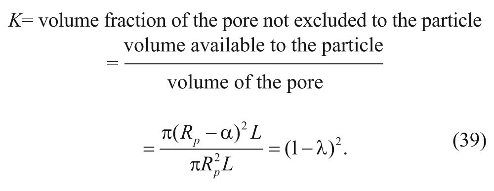
Goodman and coworkers, ²³ on the other hand, calculated the effective diffusion coefficient of polystyrene particles in tumor spheroids by first deriving the diffusion coefficient in the pore (D _pore ), which is reduced due to the steric and hydrodynamic interactions of the particles in the cylindrical pore, as shown in equation (36):

$$D_{pore}={(1-\lambda )}^2(1-2.1044\lambda +2.089{\lambda }^3-0.948{\lambda }^5)\cdot D_0,$$

$$D_0=\frac{k_{B}T}{6\pi \mu \alpha },$$

where D₀ is the diffusion coefficient in bulk liquid medium and is estimated by the Stokes-Einstein equation, λ is the ratio of the particle radius to the pore radius (λ = α/R _p ), k _B is the Boltzmann constant, T is the absolute temperature, and µ is the viscosity of the liquid. The first term of equation (36) can be derived from the expression for the partition coefficient, K, between the pore and the bulk as follows:

$$K=\frac{\text{volume fraction of pore not excluded to the particle}}{\text{volume fraction of bulk solution not excluded to the particle}},$$

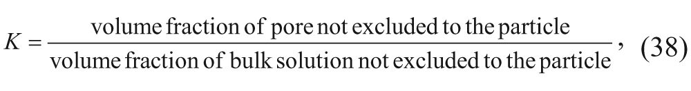
where the volume fraction in the bulk solution not excluded to the particle is assumed to be 1 since the length scale of the bulk volume is much greater than the radius of the solute. Therefore, the partition coefficient can be simplified to the volume fraction of the pore not excluded to the particle, which can be calculated by considering the steric, excluded-volume interactions between a particle and a cylindrical pore:

$$\begin{array}{c}K=\text{volume}\text{fraction}\text{of}\text{the}\text{pore}\text{not}\text{excluded}\text{to}\text{the}\text{particle}\\ =\frac{\text{volume}\text{available}\text{to}\text{the}\text{particle}}{\text{volume}\text{of}\text{the}\text{pore}}\\ =\frac{\pi {(R_p-\alpha )}^{2}L}{\pi R_p^{2}L}={(1-\lambda )}^2.\end{array}$$

The second term of equation (36) accounts for the hydrodynamic drag as the particle diffuses through the pore. The expression was generated through data fitting, ²⁸ as Beck and Schultz ²⁹ studied the diffusion of a variety of solutes across mica membranes. When the ratio of the pore diffusivity to the bulk diffusivity was plotted as a function of λ, equation (36) correlated well with their data. The pore diffusion coefficient was further reduced by the shape factor (F) that accounts for the steric hindrance in the spheroid pores and the tortuosity (τ) that leads to increased diffusion path lengths. ³⁰ Therefore, the effective diffusion coefficient can be estimated as the following expression:

$$D_{eff}=\frac{D_{pore}}{F\tau },$$

where the value for F will need to be selected from the best fit of experimental data. The value of τ can be estimated as a function of porosity based on the following expression ³¹ :

$$\frac{1}{\tau }=1-\frac{2}{3}(1+\epsilon ){(1-\epsilon )}^{\frac{2}{3}}.$$

Since Goodman and coworkers ²³ mainly investigated the effect of the nanoparticle size and the tumor architecture, the effective diffusion coefficient was simulated in detail as a function of the porosity and pore size of spheroids, as well as the size of nanoparticles. Furthermore, the spheroid was divided into a center core region, a middle region, and an outer region. The porosity and pore size for different regions were experimentally measured by imaging spheroids with negative staining.

Initial Surface Binding Sites

The number of initial surface binding sites per cell can be determined with a monolayer of cells. This number can then be converted to initial surface binding sites per tumor volume based on the radius of the cells and the porosity of spheroids. Benedetto and coworkers ³² estimated the number of integrin receptors per cell by applying excess ligands to saturate cell surface receptors with fluorescently labeled molecules. The fluorescent signal was measured and calculated to obtain the number of integrin receptors.

Goodman and coworkers ²³ used a binding kinetics model to determine the number of total surface binding sites without applying excess particles to saturate binding sites. Cells were incubated at 4 °C prior to the addition of a nanoparticle solution and during the incubation of the nanoparticle solution to inhibit endocytosis. Assuming 1:1 binding and a constant concentration of free particles, the binding and internalization of particles on a per-cell basis can be described as shown below:

$$\frac{d{N}_b}{dt}=k_a{C}_0{N}_{bs}-k_d{N}_b,$$

$$N_{bs}=B-N_b,$$

where N _b (t) is the number of particles bound per cell; N _bs (t) and B are the current and initial numbers of available binding sites per cell, respectively; and C₀ is the initial concentration of particles outside the spheroid (M). The other parameters are the same as those in equations (29) to (32). The solution of equation (42) is shown as follows:

$$N_b=\alpha (1-e^{-\gamma t}),$$

where

$$\alpha =\frac{k_a{C}_{0}B}{\gamma },$$

$$\gamma =k_a{C}_0+k_d.$$

Cells were exposed to nanoparticles at different concentrations and were allowed to achieve equilibrium. At equilibrium, equation (44) simplifies to the following expression as t tends toward infinity:

$$N_b=N_{B,eq}=\frac{K_D{C}_{0}B}{K_D{C}_0+1},$$

where K _D is the equilibrium constant,

$$K_D\equiv \frac{N_{B,eq}}{C_0{N}_{bs,eq}}=\frac{N_{B,eq}}{C_0(B-N_{B,eq})}.$$

Considering equations (47) and (48), B is the only unknown as C₀ is assumed to be constant and N _B,eq is measured as the particles are fluorescently labeled. Accordingly, B can be solved for, and B is the initial number of available binding sites.

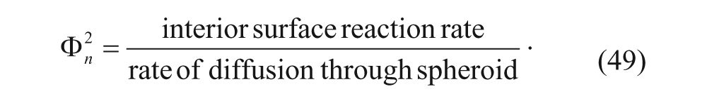
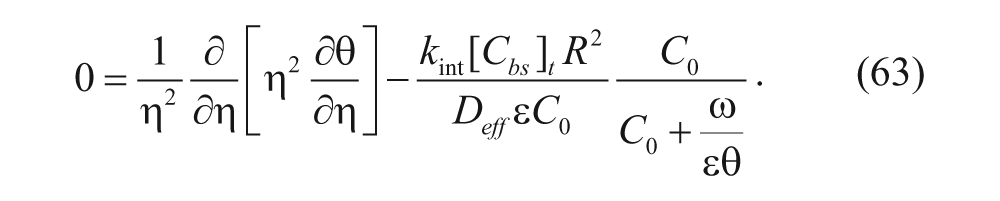
Thiele Modulus

The Thiele modulus, a dimensionless group represented by Φ _n , can also be used to determine if a vesicle system is reaction or diffusion limited without solving any ordinary differential equation (ODE) or partial differential equation (PDE), as represented below:

$${\Phi }_n^2=\frac{\text{interior surface reaction rate}}{\text{rate of diffusion through spheroid}}.$$

Thurber and Wittrup ³³ used this approach for modeling an antibody diffusing in spheroids. The approach is based on a model similar to equations (29) to (31) and assumes that the diffusion and reaction have reached steady state:

$$0=D_{eff}\frac{1}{r^2}\frac{\partial }{\partial r}\left(r^2\frac{\partial C}{\partial r}\right)-k_{a}C\cdot C_{bs}+k_d{C}_b,$$

$$0=k_{a}C\cdot C_{bs}-k_d{C}_b-k_{int}{C}_b,$$

$$0=R_s-k_{a}C\cdot C_{bs}*k_d{C}_b-k_{int}{C}_{bs},$$

where R _s is the rate of synthesis of new binding sites. The other variables are the same as those in equations (29) to (31). Dimensionless variables for the radial coordinate, free vesicles, binding sites, bound vesicles, and binding site synthesis are defined as follows:

$$\eta \equiv \frac{r}{R},$$

$$\theta \equiv \frac{C}{\epsilon C_0},$$

$$\phi \equiv \frac{C_{bs}}{{[C_{bs}]}_t},$$

$$\gamma \equiv \frac{C_b}{{[C_{bs}]}_t},$$

$$\xi \equiv \frac{R_s}{k_{int}{[C_{bs}]}_t},$$

where R is the radius of the spheroid, ϵ is the partition coefficient (which is also the fraction of tumor volume accessible to vesicles), C₀ is the vesicle concentration outside the spheroid, and [C _bs ] _t is the total number of binding sites in the spheroid divided by the spheroid volume.

Equations (50) to (52) are then nondimensionalized and simplified as follows:

$$0=\frac{1}{{\eta }^2}\frac{\partial }{\partial \eta }\left[{\eta }^2\frac{\partial \theta }{\partial \eta }\right]-\left(k_a\theta \phi -\frac{k_d}{\epsilon C_0}\gamma \right)\frac{R^2{\left[C_{bs}\right]}_t}{D_{eff}},$$

$$\gamma =\frac{\epsilon C_0}{\omega }\theta \phi .$$

$$0=\xi k_{int}-\epsilon k_a{C}_0\theta \phi *k_d\gamma -k_{int}\gamma ,$$

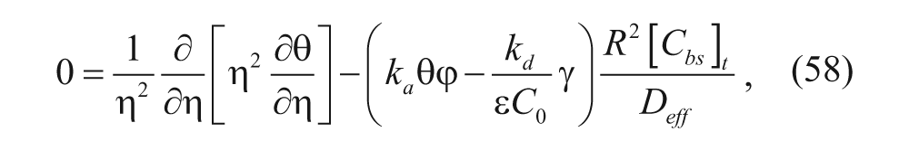
where

$$\omega =\frac{k_{int}+k_d}{k_a}.$$

Equation (59) is substituted into equation (60), and ξ is assumed to equal 1 (recall that Thurber and Wittrup ³³ assume that synthesis of new binding sites is a constant, as discussed earlier):

$$\phi =\frac{1}{\frac{\epsilon C_0\theta }{\omega }+1}.$$

Equations (59) and (62) are then substituted into equation (58) to yield

$$0=\frac{1}{{\eta }^2}\frac{\partial }{\partial \eta }\left[{\eta }^2\frac{\partial \theta }{\partial \eta }\right]-\frac{k_{\mathrm{int}}{[C_{bs}]}_t{R}^2}{D_{eff}\epsilon C_0}\frac{C_0}{C_0+\frac{\omega }{\epsilon \theta }}.$$

For a high binding affinity for the vesicles (k _a is large and ω << 1, so that C₀ >> ω/(ϵθ).

$$0=\frac{1}{{\eta }^2}\frac{\partial }{\partial \eta }\left[{\eta }^2\frac{\partial \theta }{\partial \eta }\right]-\frac{k_{\mathrm{int}}{[C_{bs}]}_t{R}^2}{D_{eff}\epsilon C_0}{\theta }^0.$$

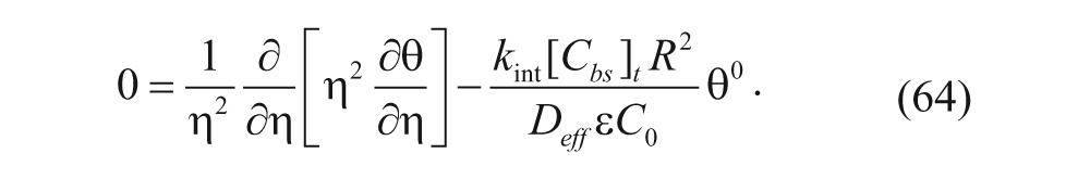
The Thiele modulus can then be defined as

$${\varphi }_n^2=\frac{k_{\mathrm{int}}{[C_{bs}]}_t{R}^2}{D_{eff}\epsilon C_0}.$$

This equation describes a net 0th-order binding regime. According to equation (65), the internalization rate becomes one of the factors that dictates whether the situation is diffusion limited or internalization limited. A large k _int gives a value of Φ _n >> 1, indicating that vesicles will experience a difficult time diffusing into spheroids. This is intuitive, since a vesicle will exhibit more difficulty reaching the core if it is easily internalized by cells on the periphery. In the model by Thurber and Wittrup, ³³ this effect is also captured when internalization occurs quickly. To keep the overall number of bound and free binding sites constant, occupied binding sites can quickly be replaced with empty binding sites, allowing more vesicles to bind to cell surface. Fewer vesicles therefore diffuse into the spheroid center.

When the binding affinity is low (k _d is large and ω >> 1), equation (63) simplifies to the following, as C₀ << ω/(ϵθ):

$$0=\frac{1}{{\eta }^2}\frac{\partial }{\partial \eta }\left[{\eta }^2\frac{\partial \theta }{\partial \eta }\right]-\frac{k_{\mathrm{int}}{[C_{bs}]}_t{R}^2}{D_{eff}\omega }\theta .$$

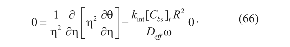
In this case, the Thiele modulus is given by

$${\varphi }_n^2=\frac{k_{\mathrm{int}}{[C_{bs}]}_t{R}^2}{D_{eff}\epsilon \omega }.$$

Compared with equation (65), this equation represents a first-order Thiele modulus, where the net binding is in the linear regime. Since ω is in equation (67), a large ω now results in a smaller Thiele modulus, leading to faster diffusion of vesicles. The Thiele modulus can also be used to predict the approximate penetration depth for a vesicle by finding the distance R for which the Thiele modulus is 1, as shown as follows ³⁴ :

$$R=\sqrt{\frac{D_{eff}\epsilon \omega }{k_{int}{[C_{bs}]}_t}}.$$

As demonstrated in equation (68), the Thiele modulus helps us to better understand the competition between binding/internalization and diffusion. However, this is merely an estimation. To obtain a detailed distribution profile, such as how many vesicles are bound and internalized, a numerical solution of the model equations is required.

Pharmacokinetics

Introduction

Pharmacokinetics is used to investigate the kinetics of drug absorption, distribution, metabolism, and elimination within the body.^35,36 To obtain quantitative values for these rates, mathematical models known as compartmental models are generally used. ³⁵ The results from a physiologically accurate pharmacokinetic model can be used to determine maximum drug delivery rates to various organs or systems and determine treatment schedules. Having this knowledge helps investigators maximize efficacy and minimize toxicity by allowing them to solve for rate constants and percent bioavailabilities, which are percentages of unchanged drug that reaches the circulation.^35,36 The most general model, and that used by many groups, is the open two-compartment model shown in Figure 4 .

Figure 4.

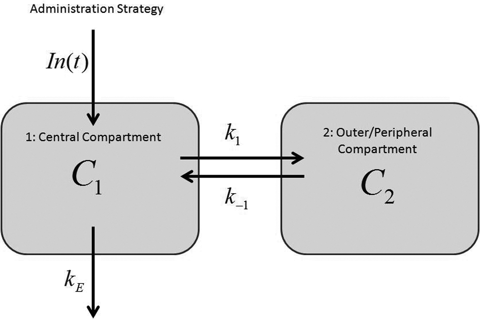
The open two-compartment model.

The central compartment is generally treated as the circulatory system, often referred to as “plasma,” and the peripheral compartment is referred to as the “tissue” that takes up most of the drug. ³⁵ In this basic setup, k _E is the elimination rate constant of drug from plasma, In(t) is the administration function for the concentration of drug over time, k₁ is the rate constant for drug distribution into the tissue from plasma, and k_–1 is the rate constant for drug distribution into the plasma from the tissue. Concentrations C₁ and C₂ are concentrations of drug in the central and peripheral compartments, respectively, and they are functions of time. Compartmental models are characterized by ODEs. For this basic model, the associated ODEs are as follows:

$$\frac{d{C}_1}{dt}=In(t)+\frac{k_{-1}{C}_2{V}_2}{V_1}-(k_1+k_E)C_1,$$

$$\frac{d{C}_2}{dt}=\frac{k_1{C}_2{V}_1}{V_2}-k_{-1}{C}_2.$$

A common administration technique used in current drug studies is that of intravenous bolus injections. In this case, no In(t) is included in the ODEs; the injection and distribution are assumed to be instantaneous. The injection is taken as an initial condition such that C₁(0) = dose/(volume of the central compartment). ³⁷

Modeling intravenous perfusion as an administration technique, Mager and Jusko ³⁷ saw success using a zero-order rate equation for In(t) such that In(t) = k/(volume of the central compartment), where k represents the 0th-order rate constant of administration. A continuous function can be used for In(t) when the experimental time period is less than the total infusion time.

For oral delivery of drugs or drug carriers, Guo et al. ³⁸ and Kim et al. ³⁹ have successfully modeled lecithin vesicle pharmacokinetics in rabbits and rats, respectively, using first-order kinetics; that is, an In(t) for these models would be given by In(t) = k * dose/(volume of central compartment). A more complicated method for modeling oral delivery used by Arangoa and coworkers ⁴⁰ will be discussed later.

With the model-defining ODEs established, the information one receives from this model would be the amount of drug in the plasma and also in the tissue as a function of time, which are found by solving the ODEs (i.e., C₁(t) or C₂(t)). This information can then be used as mentioned previously for determining optimum dosing schedules and maximum delivery rates. To find the solutions to the ODEs, nonlinear regression is often used to fit the parameters of the well-known biexponential general solution to the open two-compartment model:

$$C(t)=A_1{e}^{\alpha t}+A_2{e}^{\beta t},$$

where A₁ and α are constants dealing with the distribution of the drug or drug carrier throughout the system, and A₂ and β are constants dealing with the clearance of the drug or drug carrier from the system. ⁴¹ To solve for these solutions, nonlinear regression programs such as WinNonlin can be used by inputting sets of experimental data. ⁴²

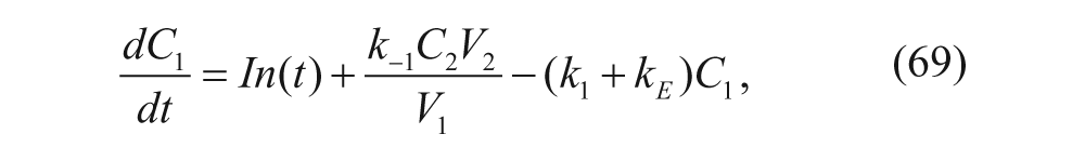
Another common method involves assuming steady state—that is, setting dc/dt=0 in the ODEs—when this assumption is applicable, such as in the liver perfusion experiments performed by Dragsten and coworkers ⁴³ that will be discussed later. In this case, equation (69) would be simplified to

$$C_1=\left(In(t)+\frac{\frac{k_{-1}{C}_2}{V_1}}{k_1+K_E}\right).$$

Although the open two-compartment model has seen success and strong agreement in a number of pharmacokinetic studies, groups have found that the accuracy of a compartmental model can increase when its compartments more closely portray the conditions present in vivo. Subsequently, cases where investigators developed their own pharmacokinetic models to achieve greater accuracy in modeling the in vivo environment will be discussed. In these cases, we will be highlighting models with consideration for administration techniques in the form of altered compartmental models, for targeting exhibited by the drug carrier, and finally for a compartment model that includes a model of a tumor being targeted. The models discussed here were developed for vesicles and polymeric nanoparticles.

Administration Method

As with the studies by Guo et al. ³⁸ and Kim et al., ³⁹ mentioned previously, there are occasions when the drug or drug carrier is not administered intravenously and therefore cannot be simply treated as instantaneously added to the central compartment. Often the drug is administered orally or through intraperitoneal injection, which is an injection into the body cavity. Arangoa et al. ⁴⁰ and Arndt et al. ⁴⁴ altered their compartmental models and found that the modifications improved the accuracy of their models in characterizing the pharmacokinetics of their delivery systems in vivo. Arndt et al. ⁴⁴ used hexadecylphosphocholine liposomes as a drug carrier that was administered first intravenously and then intraperitoneally, and they used an altered model for intraperitoneal injection. Arangoa et al. ⁴⁰ used gliadin-based nanoparticles that exhibited a strong affinity for gastrointestinal mucosa after an oral administration.

Administration Method: Intraperitoneal Injection

The hexadecylphosphocholine liposomes used by Arndt et al. ⁴⁴ were studied as a drug carrier system with both tumor-free and human breast carcinoma tumor-bearing mice. In this study, the investigators focused on the differences in pharmacokinetics between their sterically stabilized hexadecylphosphocholine liposomes, conventional liposomes, and free hexadecylphosophocholine. Performing in vivo studies, the investigators first used an intravenous injection and then an intraperitoneal injection in a separate study. When modeling the intravenous injection, the standard two-compartment model shown previously in Figure 4 was incorporated into their model (see Fig. 5 ). ⁴⁴ When modeling the intraperitoneal injection, a compartment was added to account for the peritoneal cavity; this is modeled as having one-way flow into the central cavity. ⁴⁴ The overall pharmacokinetic model incorporating both administration routes can be seen in Figure 5 .

Figure 5.

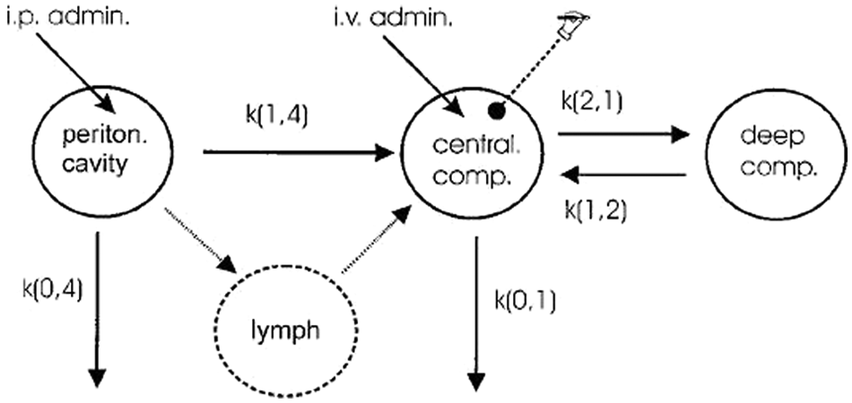
Pharmacokinetic model used by Arndt et al. ⁴⁴ to model in vivo biodistribution of liposomes. With kind permission from Springer Science+Business Media: Breast Cancer Research and Treatment, Pharmacokinetics of sterically stabilized hexade-cylphosphocholine liposomes versus conventional liposomes and free hexadecyl-phosphocholine in tumor-free and human breast carcinoma bearing mice, 58, 1999, 71-80, Arndt, D., Zeisig, R., Fichtner, I., Teppke, A. D., and A. Fahr, Figure 4.

The group used the previously mentioned WinNonlin program to perform nonlinear regression on the data. ⁴⁴ Although the authors did not provide the characteristic ODEs, we can write them following the guidelines we have previously discussed. Letting C₁ be the concentration in the central compartment, C₂ be the concentration in the deep compartment (tissue deep in the body unlike the peritoneal cavity), and C _p be the concentration in the peritoneal cavity, and denoting the compartments’ volumes with the same subscripts, the defining ODEs can be written as follows:

$$\frac{d{C}_1}{dt}=\frac{k_{(1,4)}{C}_p{V}_p}{V_1}+\frac{k_{(1,2)}{C}_2{V}_2}{V_1}-\left(k_{(2,1)}+k_{(0,1)}\right)C_1,$$

$$\frac{d{C}_2}{dt}=\frac{k_{(2,1)}{C}_1{V}_1}{V_2}-k_{(1,2)}{C}_2,$$

$$\frac{d{C}_p}{dt}=-\left(k_{(0,4)}+k_{(1,4)}\right)C_p,$$

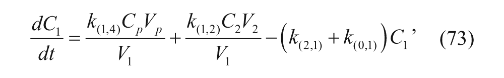
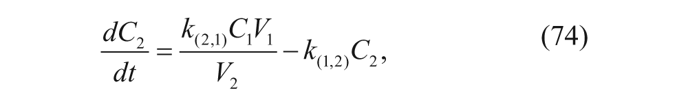
where k_(0,4) is the elimination constant from the peritoneal cavity, k_(1,4) is the rate constant for liposomes moving from the peritoneal cavity to the central compartment, k_(2,1) is the rate constant for liposomes moving from the central compartment to the deep compartment, k_(1,2) represents the reverse, and finally, k_(0,1) is the elimination constant of liposomes from the plasma. Arndt et al. ⁴⁴ used WinNonlin to determine k_(2,1), k_(1,2), and k_(0,1) for the intravenous injections first (using an open two-compartment model). These were then applied to the case where only an intraperitoneal injection was considered. ⁴⁴ The rationale for this assumption was that the physical state of liposomes was the same in plasma regardless of administration technique. That is, once the drug was in the central body compartment, the rate constants should not be affected by whether the drug was administered intravenously or intraperitoneally. Although the group found a good fit with this model, they tried to improve this model by adding the lymphatic compartment seen in Figure 5 , since the group found in literature that vesicles can pass through the lymph on their way to the plasma. ⁴⁴ As this made their model more comparable to the in vivo environment, this resulted in stronger agreement between experimental data and their pharmacokinetic model.

Arndt et al. ⁴⁴ determined pharmacokinetic rate constants by fitting their data to their model and unexpectedly discovered that their sterically stabilized liposomes experienced very similar pharmacokinetics to nonstabilized liposomes irrespective of the route of administration being intravenous or intraperitoneal.

Administration Method: Complex Oral Delivery

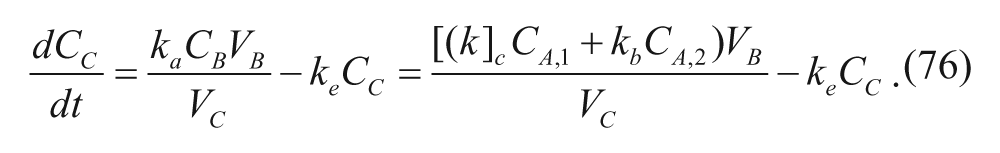
Arangoa et al. ⁴⁰ investigated the bioadhesion properties of their gliadin nanoparticles in nonhardened and cross-linked forms. The nanoparticles were loaded with carbazole as a drug substitute that could be quantified due to its fluorescence. ⁴⁰ The group decided to develop a customized compartmental model for investigation of the pharmacokinetics of the oral administration of their nanoparticles. An additional compartment denoting the gastrointestinal (GI) tract was added to the one-compartment model to take into account the nanoparticles’ adsorption to the GI wall, which results in the movement of drug from the gastrointestinal tract to the central compartment, or plasma. The investigators modeled both intravenous and oral delivery techniques. ⁴⁰ In this study, oral delivery poses an interesting case since the cargo releases into the central compartment, or plasma, differently if it is free in the gastrointestinal tract or if it is in an adhered nanoparticle. To account for this difference, two rate constants were used: one representing the absorption of free carbazole into the bloodstream and the other representing the absorption of carbazole from an adhered nanoparticle. The first rate constant, k _b , denotes a rapid release due to the quick absorption of free carbazole that came from digested (i.e., degraded) nanoparticles. The second rate constant, k _c , is a sustained-release term due to the slow release of drug from an intact nanocarrier. The model from Arangoa et al. ⁴⁰ is in Figure 6 . Note that compartment B is merely a simplification of compartment A, and therefore, k _c C_A,1+k _b C_A,2=k _a C _B . Compartment C is the central compartment, or plasma, and the elimination of carbazole from the plasma is denoted by k _e . The volumes of the compartments are denoted with matching subscripts, and the ODE to determine the concentration in the plasma of drug for this model could be written as

$$\frac{d{C}_C}{dt}=\frac{k_a{C}_B{V}_B}{V_C}-k_e{C}_C=\frac{[{(k]}_c{C}_{A,1}+k_b{C}_{A,2})V_B}{V_C}-k_e{C}_C.$$

Figure 6.

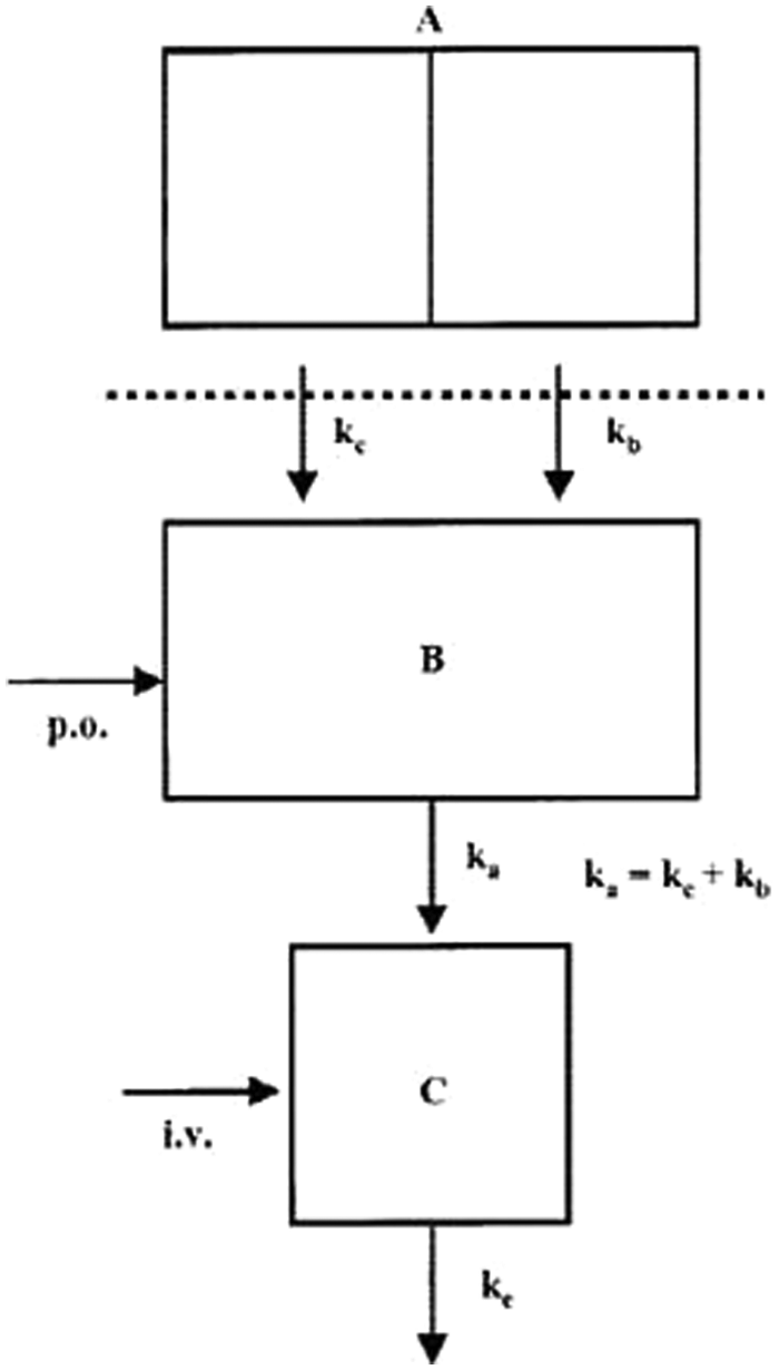
Pharmacokinetic model used by Arangoa et al. ⁴⁰ to model in vivo biodistribution of orally delivered gliadin nanoparticles. With kind permission from Springer Science+Business Media: Pharmaceutical Research, Gliadin nanoparticles as carriers for the oral administration of lipophilic drugs. Relationships between bioadhesion and pharmacokinetics, 18, 2001, 1521-1527, Arangoa, M. A., Campanero, M. A., Renedo, M. J., Ponchel, G., and J. M. Irache, Figure 1.

Targeting

As described previously, one strategy commonly used for improving drug delivery is the use of active targeting, which increases drug carrier specificity. This method has seen success in vitro and in vivo, and therefore, many studies have focused on characterizing the effects that a targeted drug carrier has on the patient. Adding specific targeting, however, will change the pharmacokinetics of the system in the body, as the drug carriers will localize in tissues that are being targeted, and compartmental models have been altered accordingly. Dragsten et al. ⁴³ used a vesicular system that incorporated galactose-containing polymers, which target the hepatic asialoglycoprotein receptor. Due to this targeting feature, the vesicles were bound to the receptors on the cell surface and then internalized as a complex, which was also accounted for in their compartmental model. ⁴³ In similar fashion, Neubauer and coworkers ⁴¹ modeled nanoparticles that target integrins in the aortic wall, and an altered compartmental model was used to account for the specific uptake at the aortic wall as well as the nonspecific uptake in the peripheral tissue.

Targeting Specific Tissue with Receptors

The vesicles used by Dragsten and coworkers ⁴³ consisted of cholesterol, dipalmitoylphosphatidylcholine, digalactosyldiacylglycerol (DGDG), and dipalmitoylphosphatidylglycerol with targeting features associated with the terminal galactose moieties on the DGDG polymers. The hepatic asialoglycoprotein receptor specifically binds galactose and is present in liver parenchymal cells. The drug carriers distributed mostly between the plasma and the liver, which was expected due to the specific targeting of the DGDG-containing vesicles. ⁴³ Accordingly, Dragsten et al. modified a standard two-compartment model to include a third compartment that corresponded to vesicle-receptor complexes that have been internalized by the liver parenchymal cells ( Fig. 7 ).

Figure 7.

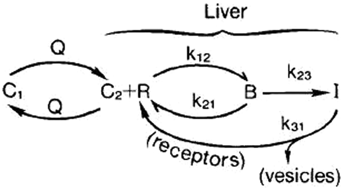
Pharmacokinetic model used by Dragsten et al. ⁴³ to model in vivo biodistribution of vesicles. Reprinted from Biochimica et Biophysica Acta, 926: 3, Dragsten, P. R., Mitchell, D. B., Covert, G., and T. Baker, Drug delivery using vesicles targeted to the hepatic asialoglycoprotein receptor, 270-279, Copyright (1987), with permission from Elsevier.

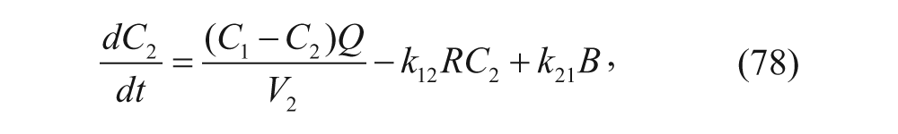
In this model, C₁ denotes the concentration of vesicles outside the liver, C₂ denotes the concentration of vesicles inside the liver, R is the concentration of unbound receptors on cell surfaces, B is the concentration of vesicle-receptor complexes on cell surfaces, and I is the concentration of vesicle-receptor complexes internalized within the parenchymal cells of the liver. Similar to the two-compartment model, rate constants define the transfer between compartments and differing states (i.e., bound vs. unbound). The exception is that the flow rate, Q, discerns the rate of plasma flow into the liver. The ODEs associated with this model can therefore be written as follows:

$$\frac{d{C}_1}{dt}=\frac{(C_2-C_1)Q}{V_1},$$

$$\frac{d{C}_2}{dt}=\frac{(C_1-C_2)Q}{V_2}-k_{12}R{C}_2+k_{21}B,$$

$$\frac{dR}{dt}=-k_{12}R{C}_2+k_{21}B+k_{31}I,$$

$$\frac{dB}{dt}=k_{12}R{C}_2-k_{21}B-k_{23}B,$$

$$\frac{dI}{dt}=k_{23}B-k_{31}I.$$

The values of the rate constants were determined with steady-state binding studies with hepatic cells and steady-state perfusion studies, as well as later confirmed with biodistribution studies. After fitting the rate constants, the complete model was used to study the effects of different doses. The model was also used to successfully predict the concentrations of drug carrier present in the liver and plasma. ⁴³

Targeting Specific Tissue While Accounting for Nonspecific Uptake

The nanoparticles used by Neubauer and coworkers ⁴¹ consisted of perfluorooctylbromide with small amounts of glycerin and a surfactant mixture. Their targeted nanoparticles contained 0.1 mol% peptidomimetic vitronectin antagonist, an integrin-targeting ligand, conjugated to polyethylene glycol (PEG)–phosphatidylethanolamine. ⁴¹ The integrin targeted by the ligand, α _V β₃, is overexpressed in connective tissue surrounding atherosclerotic vessels. The nanocarriers distributed throughout the plasma, the peripheral tissues, and the aortic wall, which was of interest due to their specific targeting. To develop a pharmacokinetic model that represented this physiological system, the investigators modified the two-compartment model by adding a third compartment ( Fig. 8 ), designated as the aortic wall. ⁴¹ Recall that based on the open two-compartment model, the peripheral compartment denotes nonspecific localization of the drug or drug carrier.

Figure 8.

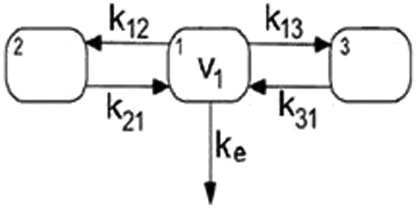
Three-compartment model used by Neubauer et al. ⁴¹ Reprinted from Magnetic Resonance in Medicine, 60:6, Neubauer, A. M., Sim, H., Winter, P. M., Caruthers, S. D., Williams, T. A., Robertson, J. D., Sept, D., Lanza, G. M., and S. A. Wickline, Nanoparticle pharmacokinetic profiling in vivo using magnetic resonance imaging, 1353-1361. Copyright (2008) Wiley-Liss, Inc.

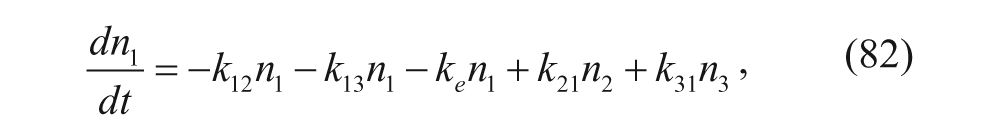
In this model, n₁ denotes the moles of nanoparticles in the plasma, n₂ denotes the moles of nanoparticles in the peripheral tissue, and n₃ is the moles of nanoparticles within the aortic wall. Volumes for the plasma, peripheral tissue, and aortic wall are denoted as V₁, V₂, and V₃, respectively. Since the equations deal with the moles of nanoparticles, the volumes of the compartments are included within the n value. V₁ was determined based on the weight of the animal, whereas V₂ and V₃ were determined through model fitting. The volumes were then used later to convert from moles to concentration. The defining ODEs can be written as follows:

$$\frac{d{n}_1}{dt}=-k_{12}{n}_1-k_{13}{n}_1-k_e{n}_1+k_{21}{n}_2+k_{31}{n}_3,$$

$$\frac{d{n}_2}{dt}=k_{12}{n}_1-k_{21}{n}_2,$$

$$\frac{d{n}_3}{dt}=k_{13}{n}_1-k_{31}{n}_3.$$

For this study, the group used in vivo data from rabbits and solved for the rate constants using nonlinear regression. Using these values, the model was found to accurately represent the biodistribution exhibited in the rabbits. Neubauer et al. ⁴¹ also were able to determine the binding rate constants for targeted and nontargeted nanoparticles, resulting in a statistically significant increase in the binding rate constant for their targeted nanoparticles.

Pharmacokinetic Modeling with Tumors

Another interesting adaptation of the standard compartment model system was performed by Schluep et al. ⁴⁵ These authors tested nanoparticles from cyclodextrin-based polymers in clinical trials for cancer treatment and investigated the pharmacokinetics of their drug carrier in 2009. To investigate pharmacokinetics in vivo, the investigators labeled individual polymers with ⁶⁴Cu before forming the nanoparticles, and positron emission tomography (PET) was then used to follow the nanocarriers through the mice. The investigators were interested in modeling the tumor pharmacokinetics and used a three-compartment model ( Fig. 9 ).

Figure 9.

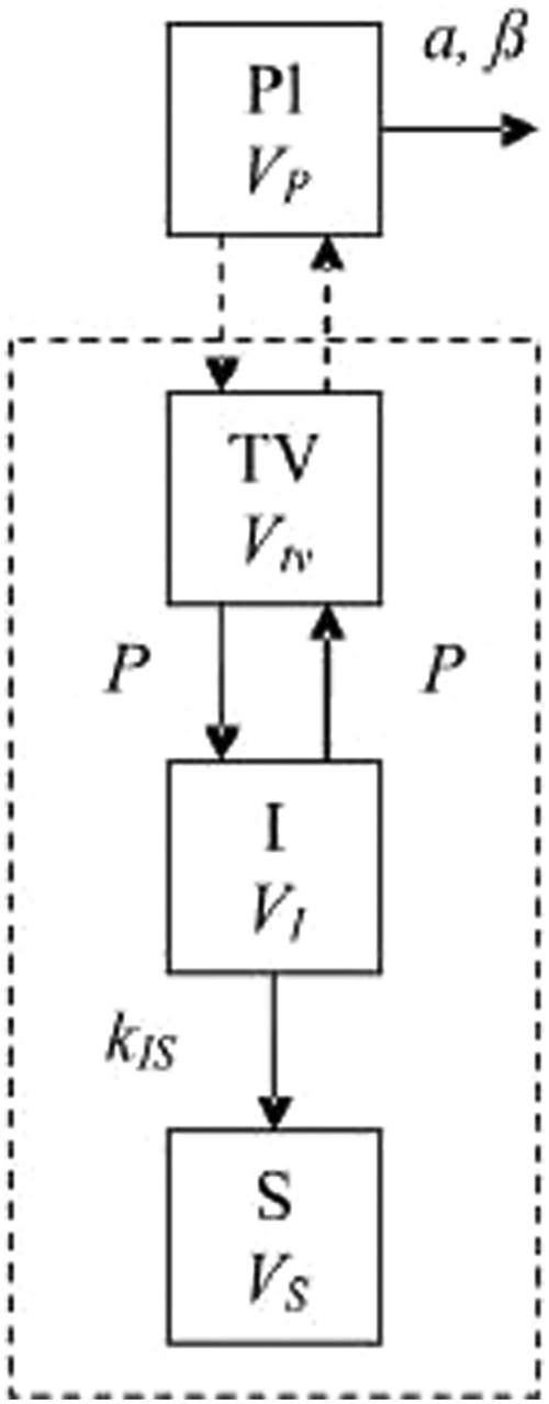
Compartmental model used by Schluep et al. ⁴⁵ Reprinted from Proceedings of the National Academy of Sciences of the United States of America, 106:27, Schluep, T., Hwang, J., Hildebrandt, I. J., Czernin, J., Choi, C. H. J., Alabi, C. A., Mack, B. C., and M. E. Davis, Pharmacokinetics and tumor dynamics of the nanoparticle IT-101 from PET imaging and tumor histological measurements, 11394-11399, Copyright (2009) National Academy of Sciences, USA.

The plasma compartment has a concentration C _pl for the polymers, and it is characterized by the biexponential function discussed previously. As mentioned earlier, the α and β parameters represent constants in the biexponential function. The nanoparticles first enter the tumor vasculature, TV, compartment. The nanoparticles then move to a compartment representing the interstitial fluid of the tumor, I. Finally, the carriers move to the S compartment, a compartment used to represent the assumption that the tumor sequesters the nanoparticles. P denotes the permeability of the nanoparticles in the tumor vasculature, and k _IS is the rate constant by which nanoparticles in the interstitial fluid of the tumor are sequestered. ⁴⁵ Since the polymers were individually labeled, the investigators recognized that the model needed to account for readings from polymers that were not part of a nanoparticle since these readings would provide data unrelated to the nanoparticle pharmacokinetics. ⁴⁵ To do so, each concentration was split into a nanoparticle term, subscript np, and a low molecular weight term, lmw. S _V denoted the surface area of the tumor vasculature, and the characteristic ODEs can be seen here:

$$\frac{d{C}_{I,lmw}}{dt}=\frac{P_{lmw}{S}_V(C_{P,lmw}-C_{I,lmw})}{V_I},$$

$$\frac{d{C}_{I,NP}}{dt}=\frac{P_{NP}{S}_V(C_{P,NP}-C_{I,NP})}{V_I}-k_{IS}{C}_{I,NP},$$

$$\frac{d{C}_{S,NP}}{dt}=\frac{k_{IS}{V}_I{C}_{I,NP}}{V_S}.$$

Schluep et al. ⁴⁵ were able to accurately model the concentrations of nanoparticles in both the tumor and the plasma when fitting parameters with their in vivo PET data. This methodology can be followed when investigators are interested in knowing the concentration of nanoparticles delivered to the tumor itself. It is important to note that various carriers will interact differently, depending on size, targeting, charge, and other parameters, and other considerations may be necessary.

In conclusion, a quantitative understanding of targeted vesicles binding to and internalizing into cancer cells, diffusing into tumors, and being cleared from the body can play a significant role in guiding efforts to optimize their design. Analysis of binding properties with radiolabeling and SPR can lead to design criteria for modifying vesicle size, number of ligands conjugated, and type of ligand conjugated. Subsequent radiolabeling experiments to determine the rate of vesicle internalization can be used in conjunction with varying the vesicle design to optimize the system. These binding and internalization properties also influence how far vesicles can penetrate into tumors. A mathematical model that incorporates the competition between diffusion into a tumor spheroid and binding/internalization into cells can accelerate the process of engineering vesicles that can enter cells to deliver their toxic payload and also penetrate into the core of the tumor. Two of the key parameters in this optimization process are the diffusion coefficient of the vesicle and the affinity of the targeting ligand. With the Wittrup model, the effect of these parameters on time integral of the antibodies bound to the receptors (inside and outside the cell) within the spheroid was calculated and used for evaluation of the antibody’s therapeutic effect on the tumor. This metric was essentially the area under the curve (AUC) for bound antibodies within the spheroid. Compartmental models for analyzing and predicting the pharmacokinetics of vesicles and their encapsulated drug can be extended to capture the targeting features of these drug carriers. This modification can lead to improved accuracy in predictions of biodistribution and the time frame over which the drug stays in the body, which are important metrics for drug delivery applications.