Covariate Selection for Estimating Individual Treatment Effects in Psychotherapy Research: A Simulation Study and Empirical Example

Abstract

Estimating individual treatment effects (ITEs) is crucial to personalized psychotherapy. It depends on identifying all covariates that interact with treatment, a challenging task considering the many patient characteristics hypothesized to influence treatment outcome. The goal of this study was to compare different covariate-selection strategies and their consequences on estimating ITEs. A Monte Carlo simulation was conducted to compare stepwise regression with and without cross-validation and shrinkage methods. The study was designed to mimic the setting of psychotherapy studies. No single covariate-selection strategy dominated all others across all factor-level combinations and on all performance measures. The least absolute shrinkage and selection operator showed the most accurate out-of-sample predictions, identified the highest number of true treatment-covariate interactions, and estimated ITEs with the highest precision across the most conditions. Domain backward stepwise regression and backward stepwise regression using Bayesian information criterion were least biased in estimating variance of ITEs across the most conditions.

Since the beginning of psychotherapy research, scientists acknowledged the problem of which patients profit from a specific treatment more than others. As early as 1905, Freud discussed characteristics that qualified or disqualified patients for psychoanalysis (Freud, 1905/2000). In his often cited article, Gordon Paul (1967) later pinpointed one of the central questions occupying psychotherapy researchers and practitioners: “What treatment, by whom, is most effective for this individual with that specific problem, and under which set of circumstances?” (p. 111). Because probably the most obvious characteristic a patient presents in treatment is his or her set of symptoms, researchers first set out to match patients with treatments by developing psychotherapeutic interventions that target a single mental disorder or a defined set of specified mental disorders (Norcross & Wampold, 2011; Zilcha-Mano, 2019). Over the last decades, great progress has been made in this field; researchers have validated and refined psychotherapeutic interventions for a wide range of mental disorders (Lambert, 2013), mostly by using randomized controlled trials (RCTs) and analyzing average treatment effects (ATEs; Z. D. Cohen & DeRubeis, 2018). However, with the progress, limitations of this approach also became apparent: On the one hand, for several mental disorders, such as depression (Barth et al., 2013) and posttraumatic stress disorder (Watts et al., 2013), it has become evident that patients—on average—benefit equally from multiple treatments (Wampold & Imel, 2015). On the other hand, the general effectiveness of psychotherapeutic treatments to date seems limited; 37% of patients still meet diagnostic criteria after treatment in the case of depression (Cuijpers et al., 2014). Although multiple treatments may be equally effective on average, patients differ substantially in how much they profit from a specific treatment (Kravitz et al., 2004; Schwartz et al., 2021; Simon & Perlis, 2010). Many factors have been considered as sources of these interindividual differences of treatment effects (Cuijpers et al., 2016; Kessler et al., 2017), commonly referred to as heterogeneity of treatment effects (Kent et al., 2020; Kravitz et al., 2004).

Personalized (or precision) medicine acknowledges these limits and tries to further individualize treatments by tailoring them to patients’ needs (Hamburg & Collins, 2010). Although there are many possibilities to adapt treatments to specific patient characteristics, an important first step within “tailor-made” psychotherapy is to discover which treatment works best for an individual patient (Cuijpers et al., 2016). Therefore, it is not a patient’s diagnosis that stands at the center of psychotherapeutic efforts, but the patient as a whole. Different approaches have been developed to achieve this goal (for a comprehensive overview, see Z. D. Cohen & DeRubeis, 2018). They all share the attempt of moving beyond the average effectiveness of treatments (a patient’s ATE) for specific diagnostic groups and try to estimate the effects of a treatment compared with another candidate treatment for single individuals (i.e., individual treatment effects [ITEs]). They also share a common challenge: finding the factors, mainly patient characteristics, that determine whether an individual profits more from one of several treatments. This challenge stands at the center of the present study, which evaluates strategies for the selection of factors (often called moderators or prescriptive factors) that influence whether a patient profits more from one treatment than another.

Individual and Conditional Treatment Effects

Consider the case of two available treatments, X = 0 and X = 1, that can be selected to treat an individual patient, U = u. Speaking in terms of the stochastic theory of causal inference (Mayer, 2019; Steyer et al., 2014), the outcome (Y $Y$ ) to be expected under both treatment conditions for this person would be E(Y|X = x, U = u). ¹ The ITE δ₁₀(u) is then defined as the difference between the expected outcomes of the two treatments for a single person (Mayer et al., 2019):

$${\delta }_{10}\left(u\right)=E\left(Y|X=1,U=u\right)-E(Y|X=0,U=u).$$

If a greater value of outcome Y indicates greater treatment success, we would choose treatment X = 1 $X=1$ for patient Joe in the case of δ₁₀(Joe) > 0.

Unfortunately, for a single subject, we can estimate the expected outcome only under one treatment condition because the outcome of getting the second treatment would be influenced by having already received the first treatment (Steyer, 2005). ² In causal inference literature, this problem is also referred to as the fundamental problem of causal inference (Holland, 1986). Consequently, ITEs can usually not be estimated directly. However, because we assume that it is not the individuals themselves who influence the treatment effect but, rather, the characteristics an individual shares with other individuals, we can approach ITEs through analyzing the expected treatment outcome conditional on treatment condition and all covariates that explain variance in the outcome (Mayer et al., 2019). If we include all covariates that determine the variability of treatment effects, ITEs δ₁₀(u) equal conditional treatment effects CE₁₀(z) (Mayer et al., 2019), which are defined as follows:

$${\mathrm{CE}}_{10}\left(z\right)=E\left(Y|X=1,Z=z\right)-E\left(Y|X=0,Z=z\right).$$

Under the assumption of conditional unit-treatment homogeneity ³ (Mayer, 2019), ITEs can thus be estimated from empirical data. More precisely, using this framework, we can estimate the treatment effect for a single individual, δ₁₀(u), by entering this individual’s values for all relevant covariates in CE₁₀(z). To put it in nonstatistical terms, instead of analyzing the effect of one treatment compared with another treatment for an individual, we analyze this effect for, for example, unmarried males with high depression scores before the beginning of treatment. Again, if a greater value of outcome Y indicates greater treatment success, we would select Treatment X = 1 for this group of patients if CE₁₀(z) > 0.

Various methods have been developed for estimating conditional treatment effects (for comprehensive overviews, see Lipkovich et al., 2017; Powers et al., 2018), all of which face the challenges of (a) modeling the functional forms of E(Y|X = 1, Z) and E(Y|X = 0, Z), either separately or combined, and (b) identifying all relevant covariates. In this study, we focus on the latter challenge using methods based on linear regression, which although are less flexible, have the advantage of being easily interpreted. A well-known approach to ITEs is the personalized advantage index (PAI). First introduced by DeRubeis et al. (2014), it has become increasingly popular in psychotherapy research in recent years (e.g., Deisenhofer et al., 2018; Huibers et al., 2015; Keefe et al., 2018; van Bronswijk, DeRubeis, et al., 2021), which is why it is of special interest in this study. The approach starts by constructing a multiple regression model that includes treatment-covariate interactions. This model is fit to a data set from which a “focal” patient is excluded (to avoid overfitting) to then predict the outcome under both treatment conditions by entering each condition and the patient’s covariate values into the model. An individual’s PAI is defined as the difference between the predicted outcomes under both treatment conditions. This procedure from model fitting to subtracting the predicted outcomes is repeated for each patient. Thus, the PAI reflects the predicted difference in outcome for a single patient. A PAI of zero implies no predicted difference in outcome between two treatments and therefore no advantage of one treatment over another for an individual patient. In contrast, a PAI of greater than or smaller than zero implies a more favorable outcome under one treatment.

Covariate Selection in Practice

In theory, all covariates interacting with treatment need to be included in a model for conditional treatment effects to equal ITEs and for correctly modeling the heterogeneity of treatment effects. However, in practice, researchers work with limited sample sizes and have to estimate which covariates are relevant and which are not. Ideally, the process of selecting covariates, including main effects and treatment-covariate interactions, is guided by subject-matter knowledge (Harrell, 2015). Because research on ITEs in psychotherapy is still in its early stages, many constructs come into consideration that may influence how an individual could react to treatment (Lorenzo-Luaces & DeRubeis, 2018). Researchers have to deal with the problem of deciding on a subset of covariates among a relatively large number of candidate variables using a relatively small sample in most studies. This increases the risk of fitting the model to idiosyncratic characteristics of the sample and thereby overfitting (Babyak, 2004; James et al., 2013). If the same model is used to predict the outcome on the basis of new data, it will likely perform badly. Therefore, although including relevant variables into the final model is justified from a theoretical standpoint, it may deteriorate predictive performance on new samples in high-dimensional settings (James et al., 2013). Including irrelevant variables, on the other hand, will always reduce accuracy of out-of-sample predictions. But with an increasing covariate-to-sample-size ratio, it becomes harder to determine which predictors are relevant and which are not. For models built with a high covariate-to-sample-size ratio, it is thus even more important to assess model performance in independent validation data.

Although most researchers seem to be aware of the role that sample size plays in the ability to identify relevant covariates, other factors are mostly neglected. Among these are the signal-to-noise ratio (SNR),

$$\mathrm{SNR}=\frac{\mathrm{Var}(f(x))}{\mathrm{Var}(ϵ)},$$

and multicollinearity among predictors. The SNR is a measure that describes the composition of the outcome variance and is related to the proportion of variance explained,

$$R^2=\frac{\mathrm{Var}(f(x))}{\mathrm{Var}(Y)}=\frac{\mathrm{SNR}}{\mathrm{SNR}+1}.$$

Because a larger residual variance leads to an increase in standard errors of parameter estimates, a lower SNR makes it harder to identify relevant covariates. Moreover, correlations, or more precisely, linear relationships (i.e., multicollinearity), between predictors lead to difficulties in estimating regression coefficients because different values for these coefficients will lead to only slight differences in the residual sum of squares. As a result, coefficient standard errors will increase, their confidence intervals will be broad, and hypothesis tests on coefficients will have low power (Fox & Fox, 2016). Because of the uncertainty in estimating coefficients, small changes in the data can lead to large changes in estimates. SNR and multicollinearity seem especially important to consider in psychotherapy research such that we expect (a) a rather limited explanatory power of our models and (b) covariates (e.g., symptoms of anxiety and depression) to be related to each other.

Current Study

To date, there is no consensus on best practices in variable selection concerning when to use which selection strategy. Therefore, the aim of the current study is to extend findings on state-of-the-art covariate-selection strategies by examining their performance with respect to estimating ITEs in psychotherapy research. We compare methods that have been used in trials on ITEs or that seem promising for this endeavor: domain backward stepwise regression (BSR; BSR-DOM), BSR using Bayesian information criterion (BSR-BIC), BSR using cross-validation (BSR-CV), forward stepwise regression (FSR) using cross-validation (FSR-CV), least absolute shrinkage and selection operator (LASSO), and group-LASSO interaction network (glinternet).

To this end, we conducted a Monte Carlo simulation that mimicked studies from psychotherapy research in factors influencing the behavior of covariate-selection strategies. These factors include sample size, SNR, correlational structure among covariates, the number of covariates, and the structure of effects (i.e., hierarchy; see below). We evaluated the performance of each covariate-selection strategy regarding the accuracy of out-of-sample predictions, the identification of treatment-covariate interactions, and the estimation of ITEs. Thereby, we hope to give researchers some guidance in their choice of a covariate-selection strategy in the context of psychotherapy research, especially when it comes to estimating ITEs, and raise awareness for the factors that need to be considered when making that choice.

Given the artificiality of the data-generating process, results from simulation studies may be difficult to translate to empirical settings. Therefore, we exemplify the ramifications of selecting a covariate-selection strategy on estimating ITEs in a real-world empirical example for which data have been made openly accessible (Huibers et al., 2015). We reanalyzed data from an RCT analyzing ITEs of cognitive therapy (CT) and interpersonal therapy (IPT) and interpreted our results in light of the findings of our simulation study.

Method

Covariate-selection strategies

Stepwise selection

Stepwise selection exists in varying forms that follow approaches based on either null hypothesis testing (NHT) or information theory (IT; Hastie et al., 2009; Mundry, 2011). Forward stepwise selection starts with an empty model containing only an intercept. Approaches following NHT at each step of the algorithm add the variable that improves model fit the most and stop when model fit does not improve significantly anymore (Mundry & Nunn, 2009). IT-based procedures also add the variable that improves model fit the most but build k models that are subsequently compared with each other using a criterion such as Akaike information criterion (AIC) or BIC (James et al., 2013). Backward stepwise selection works in the opposite direction: These procedures start with a full model (including all variables), sequentially drop the variable whose exclusion leads to the smallest (nonsignificant) decrease in model fit, and either stop when this drop in model fit becomes significant (NHT approach) or the null model is reached to eventually compare all models by some IT-based criteria (IT approach). Combinations of both forward and backward selection are used as well (James et al., 2013; Miller, 2002).

Stepwise-selection methods have been the subject of extensive criticism. Most importantly, they are a prime example of multiple testing (Harrell, 2015; Mundry & Nunn, 2009; Smith, 2018; Whittingham et al., 2006). Simulation studies have shown that models built with stepwise-selection procedures tend to include many irrelevant variables and exclude relevant variables (Derksen & Keselmann, 1992). Because of overfitting, solutions derived by stepwise procedures tend to be unstable, which means slight changes in the data result in large changes of model parameters (Mundry, 2011). An advantage of using AIC or BIC over “traditional” NHT approaches is that it is equal to using less restrictive p values (Harrell, 2015) and thereby suffers less likely from the exclusion of relevant covariates. Despite these deficiencies, stepwise-selection procedures or modifications thereof are still used within psychology. We chose to examine BSR-BIC in this study to compare it with the special form of BSR described next.

Domain stepwise selection

Fournier et al. (2009) presented a modification of classical BSR procedures developed especially for identifying prescriptive factors that was also used by Huibers et al. (2015): The authors grouped all candidate variables into domains, probably according to some criteria of substantial similarity. Within each domain, the algorithm starts with a full model that contains main effects of treatment, domain variables, and interactions between both. Variables are successively removed from this model with a decreasing α level, whereas the treatment main effect, the effect of baseline outcome, and any main effects corresponding to significant interactions are carried along irrespective of p values. We term this approach BSR-DOM in this study. The algorithm includes the following steps within each domain:

1. Build full-regression model, keep variables significant at a threshold of α = .2, build a new model with remaining variables.

2. Keep variables significant at a threshold of α = .1, build a new model with remaining variables.

3. Keep variables significant at a threshold of α = .05.

After those steps are taken within each domain, the remaining variables from each domain are combined into a single model.

Theoretically, the deficiencies of standard stepwise-regression procedures described above pertain to this modification at a somewhat lesser degree. Fournier et al. (2009) also conducted multiple tests on a single data set, which increases the likelihood of finding spurious effects, as acknowledged by the authors. However, the starting α level of .2 follows recommendations of increasing the α level because the benefit of finding relevant variables is supposed to outweigh the cost of including irrelevant variables (Babyak, 2004).

Stepwise selection using k-fold cross-validation

Another modification of stepwise selection is based on cross-validation. Using cross-validation, researchers partition the data into training and test sets. The models to be evaluated are fit on the training data, predictions are then made for the remaining observations in the test set, and all models are compared through their test error (typically estimated by mean squared error [MSE]; James et al., 2013). More precisely, the sample is split into k groups. For each model, the test MSE for group k is computed with the model being fit to the rest of the sample (i.e., not including observations from group k). This is repeated k times. The test MSE is averaged, and the model is selected that has the smallest estimated test MSE (James et al., 2013). In cases in which the number of groups k is smaller than the sample, the procedure is called k-fold cross-validation.

K-fold cross-validation is combined with stepwise selection by conducting forward (or backward) selection within each training set, which means repeatedly adding (or removing) the variable that best improves (or least worsens) model fit for this training set until the full (or empty) model is reached. For each of the k models, the test MSE is computed on the holdout test set. After this is done for all k folds, test MSE for each model is averaged over all k iterations. The size m of the model with the smallest average test MSE is selected. Then, stepwise selection is conducted on the whole data set up to size m, and this model of size m, fitted on the whole data set, is selected as the final model. As a result of the last step, performing stepwise selection on the whole data set, more accurate coefficient estimates are obtained.

Stepwise selection with cross-validation is not in widespread use, probably because NHT- and IT-based approaches were developed earlier and most standard statistical software offers some form of NHT- and IT-based stepwise selection. In contrast, researchers may have to program stepwise selection with cross-validation themselves because it is not implemented in many statistical packages. However, this procedure has the important advantage of avoiding many of the problems described above. Most importantly, it prevents from overfitting by applying a direct estimate of test MSE (James et al., 2013) and does not rely on as many assumptions as information theory criteria, which makes it applicable to a lot of frameworks (Arlot & Celisse, 2010). Hastie et al. (2017) found that stepwise selection with cross-validation is a serious contender for other advanced machine-learning approaches, such as LASSO, regarding prediction accuracy, especially in high SNR scenarios. We included both FSR-CV and BSR-CV.

LASSO

LASSO (Tibshirani, 1996) is part of a variety of shrinkage methods. In linear regression, these methods add a “penalty” to the ordinary least squares (OLS) estimator that shrinks the estimated coefficients toward zero. For LASSO, this penalty is

$$\lambda {\sum }_{j=1}^p\left|{\beta }_j\right|,$$

in which β _j denotes the regression coefficients and λ controls the effect of the penalty (Hastie et al., 2015): λ = 0 will nullify this penalty and lead to OLS estimates of the coefficients. However, if λ is large enough, the penalty will not only shrink estimates toward zero but also lead to estimates being set to zero so that LASSO offers a method for automated variable selection. Despite underestimating model parameters, LASSO leads to models with good prediction accuracy (e.g., models without overfitting) because of the bias-variance trade-off (Hastie et al., 2015): Although the penalty introduces bias for λ = 0, it also leads to a decrease in variance that can lead to a higher prediction accuracy than OLS models. Researchers thus have to find the right λ that delivers the best bias-variance trade-off that results in a low test MSE (i.e., prediction accuracy; James et al., 2013). The λ that yields the model with the highest prediction accuracy is usually chosen by estimating the test MSE via cross-validation.

LASSO has become a quite popular method because it combines good prediction accuracy with automated variable selection. As mentioned above, the (possibly) favorable bias-variance trade-off of LASSO can lead to a higher prediction accuracy than other models (James et al., 2013). The advantages of LASSO go hand in hand with the drawback of producing larger models than FSR (Helwig, 2017), which means LASSO tends to include many irrelevant variables not related to the outcome. Although other methods may tend to find the exact model more often, LASSO produces a model that includes all relevant variables many times (Tibshirani, 1996). But as Su et al. (2016) showed, even when the SNR ratio is quite high, LASSO does include many false positives, which is why they came to the conclusion that LASSO is a “variable screener rather than a model selector” (p. 3). As Hastie et al. (2017) put it, LASSO is less “aggressive” than FSR, and this behavior can be favorable, but not necessarily. One important aspect to be considered in psychotherapy research is the behavior of selection strategies under strong correlation of predictors. Confronted with two correlated variables, LASSO tends to set one to zero, which can result in worse model performance than other selection methods (Helwig, 2017).

Glinternet

Interactions pose a special challenge to covariate selection because they confront researchers with the question of hierarchy (also called heredity or marginality; Bien et al., 2013): Should main effects of corresponding interactions be included in the final model? The common answer to this question is yes because excluding main effects would imply that the effect of one predictor is visible only if the other predictor is nonzero. In this context, “strong hierarchy” describes methods that include all main effects pertaining to interactions, and “weak hierarchy” refers to methods that do not necessarily include all main effects pertaining to interactions.

Glinternet (Lim & Hastie, 2015) meets the demands of models containing interactions by making use of group-LASSO (Yuan & Lin, 2006). Group-LASSO is a variant of LASSO that can be applied to models with grouped variables (e.g., categorical variables that are split into several dummy-coded variables). Group-LASSO works similarly to LASSO, but by applying the shrinkage factor, it sets whole groups of coefficient estimates to nonzero or zero (so that not only single levels of categorical variables have an effect/no effect but also all levels).

This grouping of variables applies to interaction models with hierarchy constraints as well because the inclusion of interaction effects should always be accompanied with including main effects so that main and interaction effects can be grouped. However, glinternet can include main effects in the final model without including corresponding interaction effects. Glinternet may also find interaction effects whose associated main effects are zero in the true model. In this case, these main effects are included in the final model.

Simulation results that have evaluated performance of glinternet are scarce. Mostly, studies introducing other methods for identification of interactions have used glinternet as a benchmark procedure (Bhatnagar et al., 2020; Gosik et al., 2018; Guinot et al., 2020; Haris et al., 2016; Page et al., 2020; Tibshirani & Friedman, 2018; Wu et al., 2018). Thus, these studies did not systematically evaluate glinternet.

Simulation design

Generating the data for this simulation study, we varied five factors that we assumed to influence the performance of covariate-selection strategies: sample size, SNR, multicollinearity, number of covariates, and hierarchy. We aimed at a strong resemblance in these factors with typical trials in psychotherapy research in which heterogeneity of treatment effects was studied. To this end, we carried out a small unsystematic literature review, which is described in more detail in the Supplemental Material available online. Concerning the correlation structure of covariates, a characteristic of many studies is a “clustering” of covariates into domains. For example, Huibers et al. (2015) included several measurements of psychological distress and general functioning, which were positively correlated within domains and negatively correlated across domains. Therefore, we mimicked this grouping of variables.

On the basis of the literature research, we varied the following factors:

• 1. (total) sample size (N): 75, 150, 600;

• 2. SNR: 0.43, 1 (equaling R² of .3 and R² of .5, respectively);

• 3. Correlation structure:

•  a. No correlation among covariates (relevant and irrelevant);

•  b. Correlations of ρ = .5 within two domains of relevant variables and correlations of ρ = –.3 between relevant variables of two different domains;

• 4. Number of irrelevant covariates: 15, 30, 60;

• 5. Structure of effects (hierarchy):

•  a. Strong hierarchy: 12 relevant variables have a main effect, six of which also have an interaction effect with treatment;

•  b. Weak hierarchy: six relevant variables have a main effect and an interaction effect with treatment; six variables have an interaction effect only with treatment.

According to the fifth design factor (hierarchy), the true models underlying the simulated data were:

• 5.a: $\begin{array}{l}E\left(Y|X,Z\right)={\beta }_1{Z}_1+{\beta }_2{Z}_2+\dots +{\beta }_{12}{Z}_{12}\\ +{\gamma }_1{Z}_{1}X+{\gamma }_2{Z}_{2}X+\dots +{\gamma }_6{Z}_{6}X\end{array}$

• 5.b: $\begin{array}{l}E\left(Y|X,Z\right)={\beta }_1{Z}_1+{\beta }_2{Z}_2+\dots +{\beta }_6{Z}_6+{\gamma }_1{Z}_{1}X\\ +{\gamma }_2{Z}_{2}X+\dots +{\gamma }_{12}{Z}_{12}X,\end{array}$

with ${\beta }_1=\dots ={\beta }_{12}$ = 0.5 and ${\gamma }_1=\dots ={\gamma }_{12}$ = 1, to ensure that main and interaction effects were of the same size. For a more detailed description of the simulation setup, see the Supplemental Material. By combining all factor levels, we obtained 72 conditions, for each of which 1,000 data sets were generated. These data sets were analyzed using the six covariate-selection strategies described above. All covariate-selection strategies included all possible treatment-covariate interactions as candidate variables (in addition to main effects) but no other interactions. Only BSR-DOM and glinternet met hierarchy constraints and included main effects pertaining to included interaction effects. All selection strategies that used cross-validation for model selection (BSR-CV, FSR-CV, LASSO, glinternet) were implemented with 10-fold cross-validation, as recommended by James et al. (2013). The simulation study was programmed in the R software environment (Version 3.6.3; R Core Team, 2020) with package SimDesign (Version 2.0.1; Chalmers, 2020), which offers an environment for simulation studies that is easy to use. Other packages used for this study include the leaps package (Version 3.1; Lumley, 2020), the glmnet package (Version 4.0; Friedman et al., 2010), and the glinternet package (Version 1.0.10; Lim & Hastie, 2019). The reproducible script for this simulation study and the simulation results are available at OSF (https://osf.io/u24en).

Evaluation criteria

We evaluated the performance of covariate-selection strategies with respect to three questions: (a) Which strategy leads to the most accurate out-of-sample predictions? (b) Which strategy identifies the most true interaction effects and includes the least interaction effects not existing in the population? And (c) Which covariate-selection strategy serves best for estimating ITEs?

To answer the question of which covariate-selection strategy leads to the most accurate out-of-sample predictions, an additional test sample of 500 was simulated for each data set. Using the models built by all covariate-selection strategies, we predicted the outcome in this test sample. Subsequently, we computed the test MSE on this sample as a common measure of prediction accuracy (Hastie et al., 2009). A lower test MSE indicates a smaller overall difference between predicted and actual outcomes. To translate this into our application area, a lower test MSE achieved with one covariate-selection strategy compared with another would mean that we would be better at predicting the treatment outcome for a single patient using this strategy.

To evaluate how reliable covariate-selection strategies identify treatment-covariate interactions, the proportion of true and false interaction effects included in the final model was computed. These criteria are abbreviated as TPR_IA (true positive rate of interactions) and FPR_IA (false positive rate of interactions), respectively:

$${\mathrm{TPR}}_{\mathrm{IA}}=\frac{\mathrm{number}\mathrm{of}\mathrm{included}\mathrm{true}\mathrm{interactions}}{\mathrm{number}\mathrm{of}\mathrm{true}\mathrm{interactions}}$$

$${\mathrm{FPR}}_{\mathrm{IA}}=\frac{\mathrm{number}\mathrm{of}\mathrm{included}\mathrm{false}\mathrm{interactions}}{\mathrm{number}\mathrm{of}\mathrm{false}\mathrm{interactions}}.$$

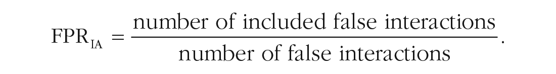
TPR_IA and FPR_IA are computed instead of the absolute number of true/false positives because the number of true treatment-covariate interactions varies with the fifth design factor (hierarchy) and the number of false treatment-covariate interactions varies with the fourth design factor (number of irrelevant covariates).

Considering the precision of estimated ITEs, we first had to estimate ITEs using covariate-selection strategies. This was achieved by simply using the models built with these strategies to estimate the outcome under both treatment conditions for each simulated observation (from the sample used to build the models) and then computing the difference between both predicted treatment outcomes as an estimate for δ(u). Because we used simulated data, the true ITEs are known. As a measure for precision of that estimate, we chose root-mean-square error (RMSE) of true and estimated ITEs:

$$\mathrm{RMSE}(\widehat{\delta }(u))=\sqrt{\frac{1}{N}{(\delta (u)-\widehat{\delta }(u))}^2}.$$

This measure can be thought of as the average deviation between true and estimated ITEs. To put the absolute size of the $\mathrm{RMSE}\left(\widehat{\delta }\right(u))$ into context, one can consider the distribution of true ITEs. In our simulation, true ITEs were normally distributed with $\sigma \left(\delta \left(u\right)\right)$ , depending on hierarchy and multicollinearity: For strong hierarchy and no multicollinearity, $\sigma \left(\delta \left(u\right)\right)$ = 2.45; for weak hierarchy and no multicollinearity, $\sigma \left(\delta \left(u\right)\right)$ = 3.46; for strong hierarchy and multicollinearity, $\sigma \left(\delta \left(u\right)\right)$ = 3.6; and for weak hierarchy and no multicollinearity, $\sigma \left(\delta \left(u\right)\right)$ = 3.8. For example, in scenarios with weak hierarchy and no multicollinearity, $\mathrm{RMSE}\left(\widehat{\delta }\left(u\right)\right)$ = 1 would imply that, on average, estimated ITEs differ 0.29 SD from true ITEs.

In addition, the relative bias of the variance of estimated ITEs was computed. The variance of ITEs, $\mathrm{Var}\left(\delta \left(u\right)\right)$ , is a measure of the heterogeneity of treatment effects and indicates how much individuals differ in their response to treatment. Large differences in this responsiveness (i.e., high $\mathrm{Var}\left(\delta \left(u\right)\right)$ ) would imply that patients could profit a great deal from allocation to their optimal treatment, whereas small differences (i.e., small $\mathrm{Var}\left(\delta \left(u\right)\right)$ ) would imply only small gains as a result of this allocation. Therefore, although precisely estimating ITEs is important for correctly allocating individuals to their optimal treatment, overestimating or underestimating $\mathrm{Var}\left(\delta \left(u\right)\right)$ could lead to erroneous conclusions about the practical relevance of personalizing treatment allocations.

Data analysis

Five full factorial analyses of variance (ANOVAs) were conducted to test for main and interaction effects of all factors on all evaluation criteria (selection strategy, SNR, sample size, correlation, number of irrelevant covariates, hierarchy). ANOVAs were modeled to include all higher order interaction effects (up to the six-way interaction of all factors), but the focus of interpretation laid on main effects and interactions with covariate-selection strategy. For every ANOVA, assumptions of normality and homogeneity of variance were checked by inspecting “residuals versus fitted values” plots and Q-Q plots (Fox & Fox, 2016). For each evaluation criteria, all main effects and interaction effects with covariate-selection strategy were statistically significant at the .05 significance level (for detailed results, see Tables S1 to S5 in the Supplemental Material). However, because of the large sample size, “significance” of results should not be overinterpreted (J. Cohen, 1994). Instead, the focus in interpreting results lies on the effect size η² (Table 1) and a visual inspection of effects. Only effects with η² ≥ .001 and up to three-way interactions with covariate-selection strategy are reported in the text. In addition, the median for each evaluation criterion in each condition was computed and compared between covariate-selection strategies.

Table 1.

Effect Sizes (η²) for Main Effects and Interactions With Covariate-Selection Strategy

Factor	Evaluation criteria
	Prediction accuracy	TPRIA	FPRIA	Estimated ITE	Bias of variance
Method	.011	.081	.264	.036	.165
N	.119	.539	.056	.588	.027
SNR	.608	.049	.009	.086	< .001
Multicollinearity	.141	.018	.004	.014	.002
Irrel cov	.003	.013	.061	.011	.011
Hierarchy	< .001	.013	< .001	.042	.008
Method × Sample Size	.006	.021	.050	.014	.040
Method × SNR	.001	.001	.011	.002	.013
Method × Multicollinearity	.001	.005	.009	.003	.002
Method × Irrel Cov	.001	.004	.030	.001	.020
Method × Hierarchy	< .001	.002	.001	< .001	.002
Method × N × SNR	.001	.006	.002	.003	.004
Method × N × Irrel Cov	.001	.002	.005	.001	.010
Method × N × Multicollinearity	< .001	.001	.004	.001	.001
Method × N × Hierarchy	< .001	.001	.001	.001	.001
Method × Multicollinearity × Hierarchy	< .001	.001	< .001	.001	< .001
Method × SNR × Irrel Cov	< .001	< .001	.001	.001	.001
R 2	.922	.813	.542	.827	.322

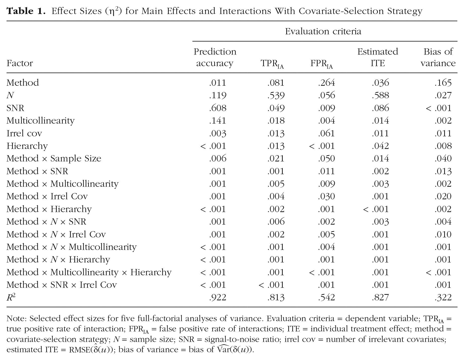
Note: Selected effect sizes for five full-factorial analyses of variance. Evaluation criteria = dependent variable; TPR_IA = true positive rate of interaction; FPR_IA = false positive rate of interactions; ITE = individual treatment effect; method = covariate-selection strategy; N = sample size; SNR = signal-to-noise ratio; irrel cov = number of irrelevant covariates; estimated ITE = $\mathrm{RMSE}(\widehat{\delta }(u))$ ; bias of variance = bias of $\widehat{\mathrm{Var}}(\delta \left(u\right))$ .

Results

Analysis of extreme values

An analysis of extreme values showed that a lot of extreme values occurred for BSR-BIC when the sample size was small (N = 75). These values were in some cases so extreme (more than a thousand times higher than the median) that the decision was made to exclude this covariate-selection strategy from the ANOVAs. Because results for larger sample sizes were comparable with other methods, BSR-BIC was included in plots. For all other conditions and covariate-selection strategies, no other extreme values occurred (except for a single iteration with BSR-DOM that was excluded).

Accuracy of out-of-sample predictions

Several main effects and interactions with covariate-selection strategy showed effect sizes of η² ≥ .001: SNR yielded a large effect, η² = .608; correlation yielded η² = .141 sample size yielded η² = .119; covariate-selection strategy yielded η² = .011; and number of irrelevant covariates yielded η² = .003. Furthermore, the interaction of selection strategy with sample size yielded η² = .006, the interaction of selection strategy with SNR yielded η² = .001, the interaction of selection strategy with number of irrelevant covariates yielded η² = .001, and the interaction of selection strategy with correlation yielded η² = .001. In addition, the three-way interactions of covariate-selection strategy, sample size, and SNR and covariate-selection strategy, sample size, and number of irrelevant covariates both yielded η² = .001. Overall, the model accounted for 92.2% of variance in the dependent variable (R² = .922; Table 1).

A visual inspection of direction and size of effects revealed that a lower SNR, a lower sample size, a higher number of irrelevant covariates, and correlation among predictors led to visible worse out-of-sample predictions for all covariate-selection strategies. Furthermore, reflecting the interactions of covariate-selection strategy with sample size and with SNR, we found that differences between strategies diminished as sample size and SNR increased (for details, see Figs. S1–S5 in the Supplemental Material).

To more precisely answer the question of which covariate-selection strategy leads to the most accurate out-of-sample predictions, median test MSE was computed in all design cells and compared among covariate-selection strategies (see Table 2). LASSO had the lowest median test MSE in 55.6% of conditions, most of which were characterized by a sample size of 75 or 150. Glinternet had lowest test MSE in 27.8% of conditions, all of which were characterized by strong hierarchy. FSR-CV, BSR-CV, and BSR-BIC had the lowest test MSE in 5.6%, 5.6%, and 4.2% of conditions, respectively, all of which were characterized by a sample size of 600 and a high SNR. BSR-DOM had the lowest test MSE in one condition, characterized by a sample size of 600, a low SNR, no correlation, and 15 irrelevant covariates. However, reflecting the small effect size of covariate-selection strategy, we found that differences between strategies in out-of-sample prediction accuracy were rather small in some conditions, especially in high sample sizes.

Table 2.

Performance of Different Covariate-Selection Strategies Across Conditions

Evaluation criterion	Method
	BSR-DOM	BSR-BIC	BSR-CV	FSR-CV	LASSO	Glinternet
Prediction accuracy	1.4%	4.2%	5.6%	5.6%	55.6%	27.8%
Highest median TPRIA
Ignoring ties	18.1%	22.2%	15.3%	19.4%	87.5%	41.7
Sole first place	—	11.1%	1.4%	—	40.3%	—
Median(FPRIA) = 0 a	0%	37.5%	76.4%	70.8%	0%	16.7%
Precision of estimated ITE	0%	4.2%	8.3%	5.6%	72.2%	9.7%
Bias of variance	40.3%	34.7%	4.2%	20.8%	0%	0%

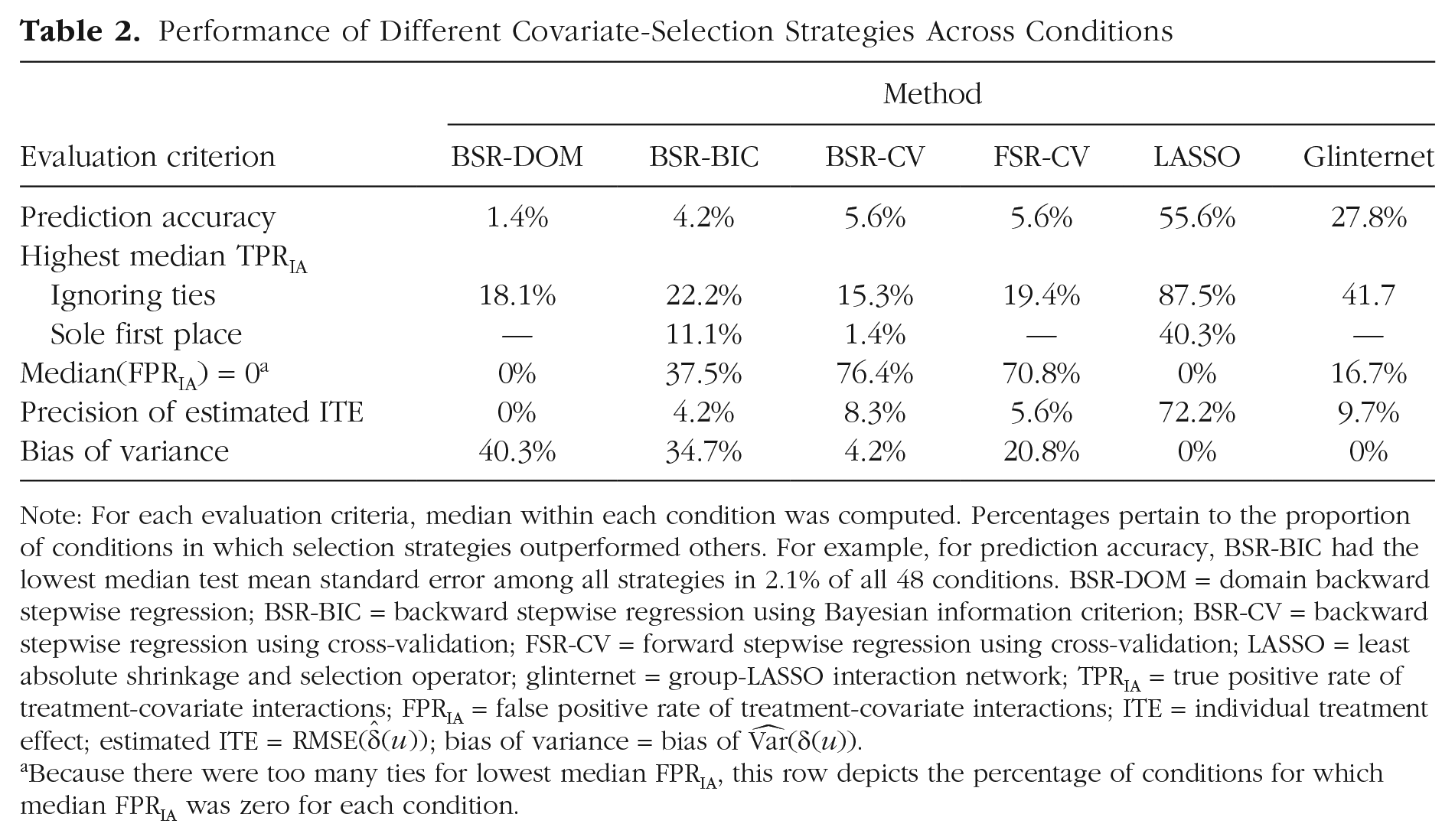
Note: For each evaluation criteria, median within each condition was computed. Percentages pertain to the proportion of conditions in which selection strategies outperformed others. For example, for prediction accuracy, BSR-BIC had the lowest median test mean standard error among all strategies in 2.1% of all 48 conditions. BSR-DOM = domain backward stepwise regression; BSR-BIC = backward stepwise regression using Bayesian information criterion; BSR-CV = backward stepwise regression using cross-validation; FSR-CV = forward stepwise regression using cross-validation; LASSO = least absolute shrinkage and selection operator; glinternet = group-LASSO interaction network; TPR_IA = true positive rate of treatment-covariate interactions; FPR_IA = false positive rate of treatment-covariate interactions; ITE = individual treatment effect; estimated ITE = $\mathrm{RMSE}\left(\widehat{\delta }\right(u))$ ; bias of variance = bias of $\widehat{\mathrm{Var}}\left(\delta \left(u\right)\right)$ .

a

Because there were too many ties for lowest median FPR_IA, this row depicts the percentage of conditions for which median FPR_IA was zero for each condition.

Identification of interactions with treatment

TPR_IA

The main effect of sample size yielded the largest effect size (η² = .539), followed by covariate-selection strategy (η² = .081), SNR (η² = .049), correlation among predictors (η² = .018), number of irrelevant covariates (η² = .013), and hierarchy (η² = .013). Of all interaction effects with covariate-selection strategy, the interaction with sample size showed the largest effect (η² = .021), followed by correlation (η² = .005), number of irrelevant covariates (η² = .004), hierarchy (η² = .002), and SNR (η² = .001). Furthermore, five three-way interactions with covariate-selection strategy exhibited an effect of η² = .001: sample size and SNR (η² = .006), sample size and number of irrelevant covariates (η² = .002), sample size and correlation (η² = .001), ( ${\eta }^2=.001$ ), sample size and hierarchy (η² = .001), and correlation and hierarchy (η² = .001). Overall, the model accounted for 81.3% of variance in the dependent variable (R² = .813; Table 1).

Visual inspection (see Figs. S6–S10 in the Supplemental Material) of all two-way interactions with covariate-selection strategy indicated that a lower SNR, a lower sample size, correlation among predictors, higher number of irrelevant covariates, and weak hierarchy were associated with a lower TPR_IA. Figure 1 visualizes the effect of SNR and sample size on TPR_IA, depending on covariate-selection strategy. The relative performance pertaining to TPR_IA of covariate-selection strategies changes with SNR and sample size: For example, for a low SNR and sample size of 75, BSR-DOM outperforms glinternet, whereas glinternet performs better than BSR-DOM in conditions with high SNR and a sample size of 150. A special mention should be made of the wide distributions of some covariate-selection strategies in some conditions. For example, for a high SNR and large sample size, with BSR-DOM, researchers would be able to identify all interaction effects in 50% of cases simulated in this study, but in 25% of cases, the TPR_IA is less than .75.

Fig. 1.

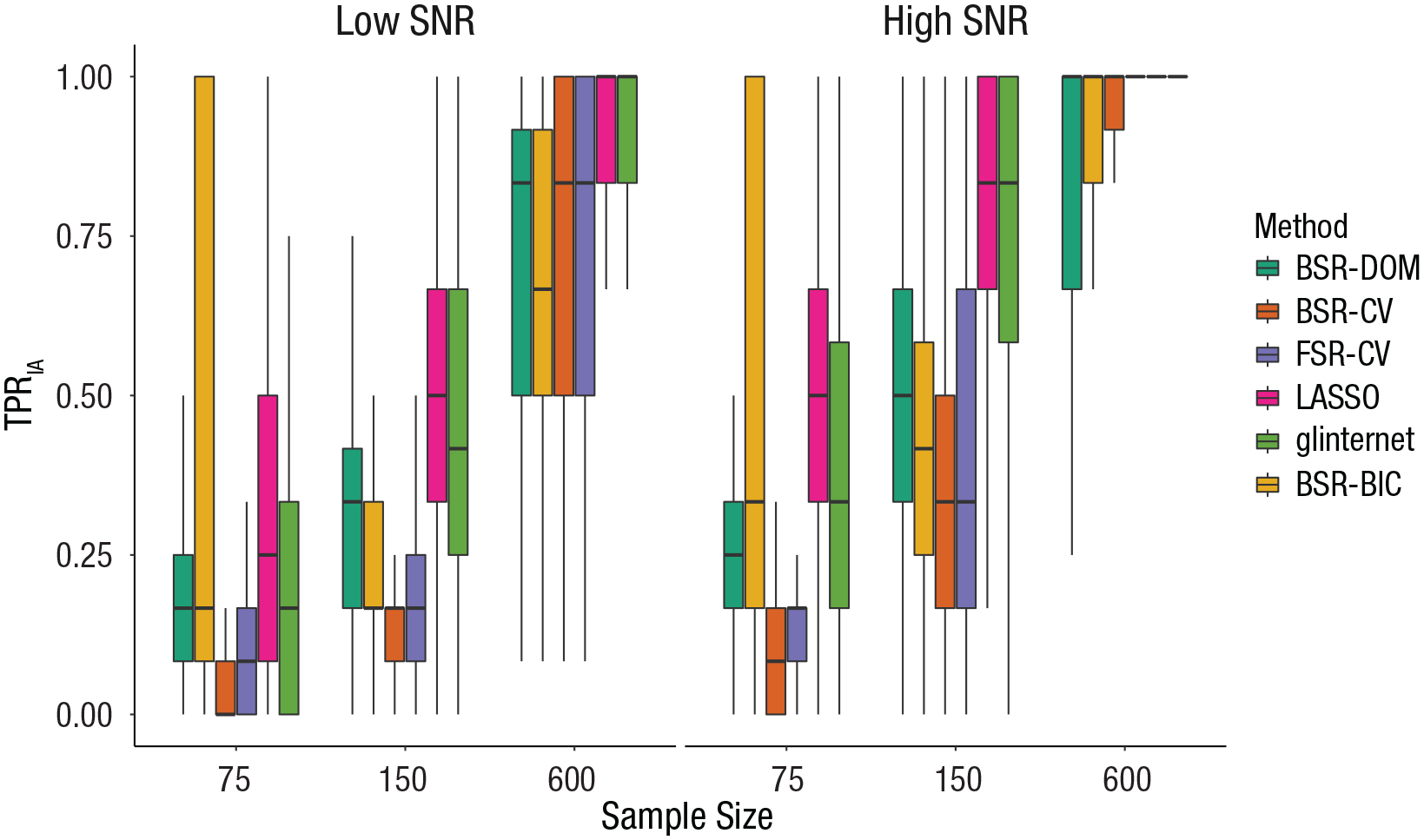
Effect of covariate-selection strategy, sample size, and signal-to-noise ratio (SNR) on the true positive rate of interactions (TPR_IA). The boxes represent the interquartile range (IQR), and the horizontal lines in the boxes represent the median. The whiskers represent values that fall outside the IQR but within 1.5× the IQR. BSR-DOM = domain backward stepwise regression (original analysis strategy from Huibers et al., 2015); BSR-CV = backward stepwise regression using cross-validation; FSR-CV = forward stepwise regression using cross-validation; LASSO = least absolute shrinkage and selection operator; glinternet = group-LASSO interaction network; BSR-BIC = backward stepwise regression using Bayesian information criterion.

In 40.3% of conditions, LASSO had the highest median TPR_IA, most of which were characterized by a sample size of 150 (see Table 2). In 11.1% of conditions, BSR–BIC had the highest TPR_IA, all of which were characterized by a sample size of 75. In 1.4% of conditions, BSR–CV had the highest TPR_IA. In 20.8% of conditions, LASSO and glinternet both had the highest median TPR_IA, most of which were characterized by a strong hierarchy. In 2.8% of conditions, LASSO and BSR–DOM had the highest median TPR_IA (in which sample size was 75). In 1.4% of conditions, LASSO and BSR-CV had the highest median TPR_IA. There were more than two selection strategies tied at first place for TPR_IA in 22.2% of conditions, most of which were characterized by a sample size of 600.

FPR_IA

The main effect of covariate-selection strategy yielded the largest effect size (η² = .264), followed by the number of irrelevant covariates (η² = .061), sample size (η² = .056), SNR (η² = .009), and correlation (η² = .004). Furthermore, all interactions with covariate-selection strategy had noteworthy effect sizes: The interaction of covariate-selection strategy with sample size yielded η² = .050, the interaction of covariate-selection strategy with the number of irrelevant covariates yielded η² = .030, the interaction of covariate-selection strategy with correlation among predictors yielded η² = .009, the interaction of covariate-selection strategy with SNR yielded η² = .011, and the interaction of covariate-selection strategy with hierarchy yielded η² = .001. In addition, five three-way interactions with covariate-selection strategy exhibited an effect of η² ≥ .001, sample size and SNR (η² = .002),, sample size and number of irrelevant covariates (η² = .005), sample size and correlation (η² = .004), sample size and hierarchy (η² = .001), and SNR and number of irrelevant covariates (η² = .001). Overall, the model accounted for 54.2% of variance in the dependent variable (R² = .542; Table 1).

A visual inspection of direction and size of effects revealed that the effects of all factors differed considerably in dependence of covariate-selection strategy (see Figs. S11–S15 in the Supplemental Material). The lower part of Figure 2 shows the effect of sample size and SNR on FPR_IA, depending on covariate-selection strategy. For LASSO and glinternet, FPR_IA rises with a growing sample size and an increasing SNR. For BSR-DOM, the number stays constant. For BSR-CV and FSR-CV, FPR_IA increases slightly with the sample size but not the SNR.

Fig. 2.

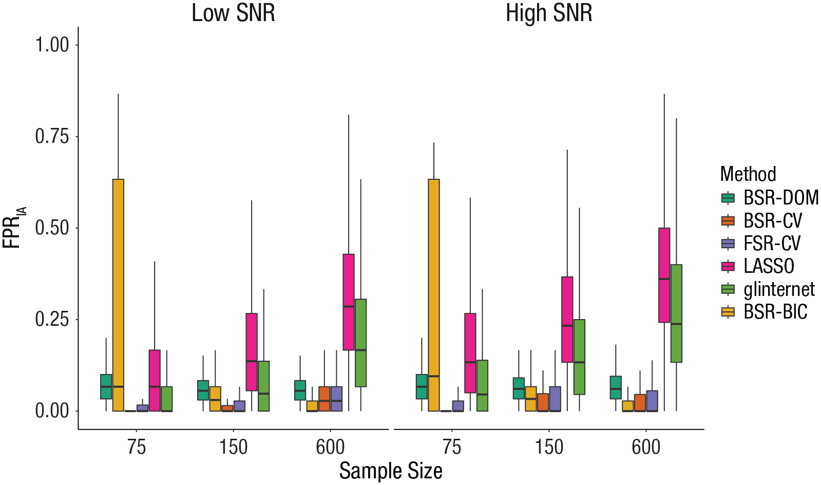
Effect of covariate-selection strategy, sample size, and signal-to-noise ratio (SNR) on the false positive rate of interactions (FPR_IA). The boxes represent the interquartile range (IQR), and the horizontal lines in the boxes represent the median. The whiskers represent values that fall outside the IQR but within 1.5× the IQR. BSR-DOM = domain backward stepwise regression (original analysis strategy from Huibers et al., 2015); BSR-CV = backward stepwise regression using cross-validation; FSR-CV = forward stepwise regression using cross-validation; LASSO = least absolute shrinkage and selection operator; glinternet = group-LASSO interaction network; BSR-BIC = backward stepwise regression using Bayesian information criterion.

To answer the question of which strategy was associated with the smallest/highest FPR_IA, we took a closer look at median FPR_IA of all strategies in each condition (see Table 2). BSR-CV and FSR-CV clearly had the lowest FPR_IA across conditions; median FPR_IA was 0 in 76.4% and 70.8% of all conditions, respectively. BSR-BIC had a median FPR_IA of 0 in 37.5% of all conditions, most of which were characterized either by a sample size of 75 and a large number of irrelevant variables or by a sample size of 600 and a low number of irrelevant variables. Glinternet also had a median FPR_IA of 0 in 16.7% of conditions, all of which were characterized by a sample size of 75. But as Figure 2 shows, median FPR_IA of glinternet could rise considerably above that of BSR-DOM, FSR-CV, and BSR-CV in larger sample sizes. LASSO had the highest median FPR_IA in 75% of conditions, BSR-DOM had the highest median FPR_IA in 5.6% of conditions, and BSR-BIC had the highest median FPR_IA in 10% of conditions.

Estimation of ITEs

Precision of estimated ITEs

The main effect of sample size yielded the largest effect size (η² = .588), followed by SNR (η² = .086), hierarchy (η² = .042), covariate-selection strategy (η² = .036), correlation among predictors (η² = .014), and number of irrelevant covariates (η² = .011). The interaction of covariate-selection strategy with sample size yielded η² = .014, the interaction of covariate-selection strategy with correlation yielded η² = .003, the interaction of covariate-selection strategy with SNR yielded η² = .002, and the interaction of covariate-selection strategy with number of irrelevant covariates yielded η² = .001. Furthermore, six three-way interactions with covariate-selection strategy exhibited an effect of η² ≥ .001: sample size and SNR (η² = .003), sample size and correlation (η² = .001), sample size and number of irrelevant covariates (η² = .001), sample size and hierarchy (η² = .001), SNR and number of irrelevant covariates (η² = .001), and correlation and hierarchy (η² = .001). Overall, the model accounted for 82.7% of variance in the dependent variable (R² = .827; Table 1).

Visualization of all two-way interactions with covariate-selection strategy (see Figs. S16–S20 in the Supplemental Material) showed that a smaller sample size, a lower SNR, correlation among predictors, a higher number of irrelevant covariates, and weak hierarchy led to an increase in $\mathrm{RMSE}\left(\widehat{\delta }\right(u))$ , which means that predictions of ITEs generally became less accurate. Figure 3 shows the effects of sample size and SNR on $\mathrm{RMSE}\left(\widehat{\delta }(u)\right)$ for each covariate-selection strategy. As sample size and SNR increased, differences between selection strategies decreased. In addition, depending on sample size and SNR, the covariate-selection strategy that led to the lowest $\mathrm{RMSE}\left(\widehat{\delta }(u)\right)$ changed: For a low SNR, LASSO outperformed all other strategies for all sample sizes (averaged over all other factors), whereas for a high SNR, FSR-CV and BSR-CV had a minor advantage over LASSO.

Fig. 3.

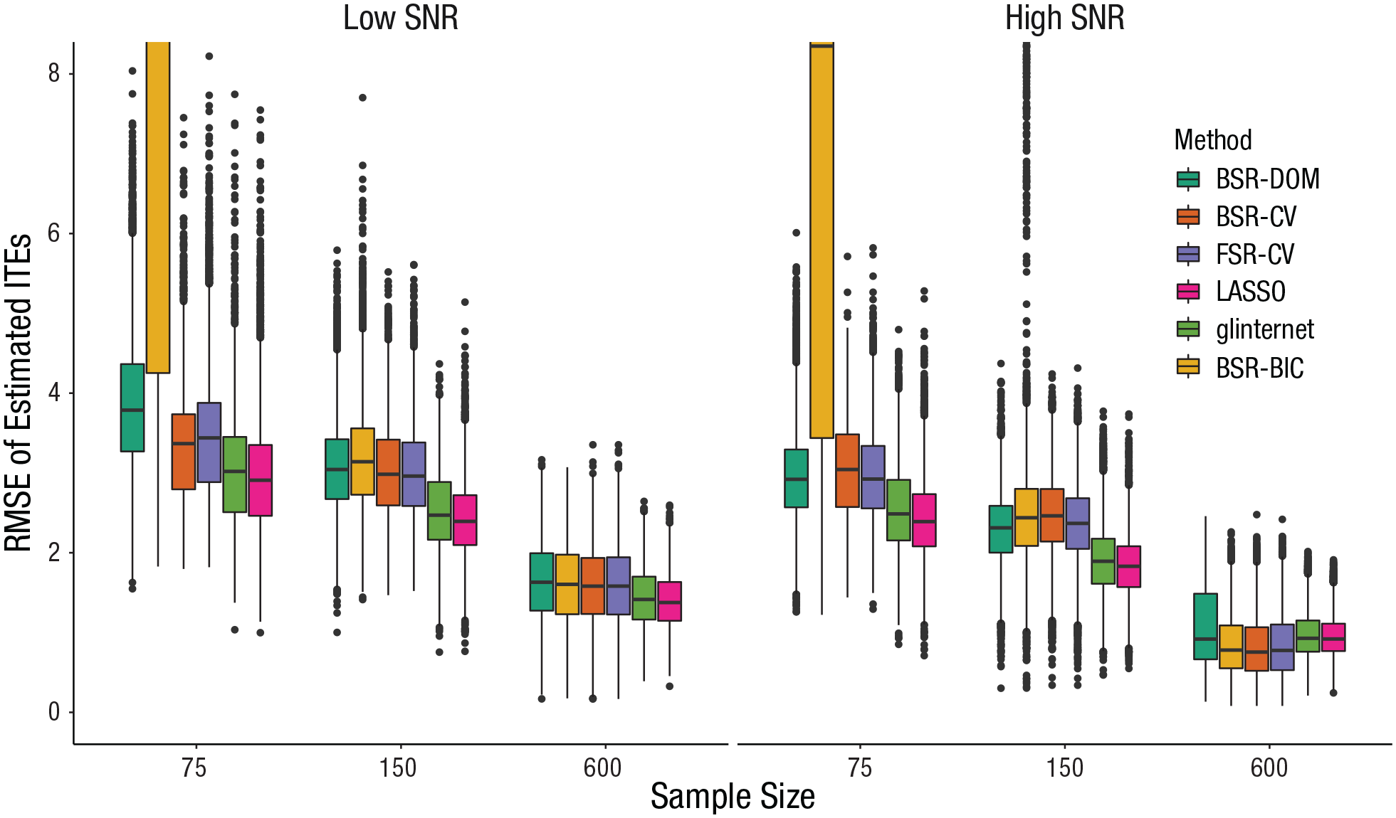
Effect of covariate-selection strategy and signal-to-noise ratio (SNR) on precision of estimated individual treatment effects (ITEs). The boxes represent the interquartile range (IQR), and the horizontal lines in the boxes represent the median. The whiskers represent values that fall outside the IQR but within 1.5× the IQR, and the dots represent outliers (values outside the IQR and beyond 1.5× the IQR). BSR-DOM = domain backward stepwise regression (original analysis strategy from Huibers et al., 2015); BSR-CV = backward stepwise regression using cross-validation; FSR-CV = forward stepwise regression using cross-validation; LASSO = least absolute shrinkage and selection operator; glinternet = group-LASSO interaction network; BSR-BIC = backward stepwise regression using Bayesian information criterion.

LASSO led to the smallest median $\mathrm{RMSE}\left(\widehat{\delta }(u)\right)$ in 72.2% of all conditions and performed especially well in small sample sizes (see Table 2). Glinternet had the smallest median $\mathrm{RMSE}\left(\widehat{\delta }(u)\right)$ in 9.7% of all conditions, all of which were characterized by strong hierarchy. BSR-CV (8.3%) and FSR-CV (5.6%) outperformed other strategies in some conditions with a sample size of 600 and a high SNR. BSR-BIC had the smallest median $\mathrm{RMSE}\left(\widehat{\delta }(u)\right)$ in 4.2% of conditions, which were characterized by a sample size of 600 and a low SNR.

Relative bias of estimated variance of ITEs

Several main effects were of notable size: Covariate-selection strategy showed the largest effect (η² = .165), sample size yielded η² = .027, number of irrelevant covariates yielded η² = .011, hierarchy yielded η² = .008, and correlation among predictors yielded η² = .002. All interactions with covariate-selection strategy exhibited effects of η² ≥ .001: The interaction with sample size yielded η² = .040, the interaction with the number of irrelevant covariates yielded η² = .020, the interaction with SNR yielded η² = .013, and the interactions with correlation and hierarchy both yielded η² = .002. In addition, five three-way interactions with covariate-selection strategy exhibited an effect of η² ≥ .001: sample size and number of irrelevant covariates (η² = .010), sample size and SNR (η² = .004), sample size and correlation (η² = .001), sample size and hierarchy (η² = .001), and SNR and number of irrelevant covariates (η² = .001). Overall, the model accounted for 32.2% of variance in the dependent variable (R² = .322; Table 1).

Visual inspection of these effects showed that using BSR-DOM, the variance of ITEs tended to be overestimated, whereas using all other strategies resulted in underestimating variance of ITEs in many cases (see Figs. S21–S25 in the Supplemental Material). With an increasing sample size and increasing SNR, relative bias shrinks toward zero for all strategies. For FSR-CV and BSR-CV, the tendency to underestimate bias in low sample sizes reverts for a sample size of 600; median relative bias of $\widehat{\mathrm{Var}}(\delta (u))$ was over zero in these cases.

Inspecting median absolute relative bias of $\widehat{\mathrm{Var}}(\delta (u))$ in all conditions revealed that in 40.3% of all conditions, BSR-DOM had the lowest median absolute relative bias; in 34.7% of conditions, it was BSR-BIC; in 20.8% of conditions, it was FSR-CV; and in 4.2% of conditions, it was BSR-CV (see Table 2). BSR-DOM performed especially well in smaller sample sizes, whereas BSR-BIC performed well in medium to large sample sizes. The conditions in which FSR-CV had the lowest median absolute relative bias were mostly characterized by a low SNR. But across simulation replications, the estimated variance of ITEs spread widely: For example, across all replications that were characterized by a sample size of 150 and a low SNR, BSR-DOM led to an overestimation of $\mathrm{Var}(\delta (u))$ in more than 50% of replications, whereas for more than 25%, it was underestimated.

Analysis of Empirical Data From Huibers et al. (2015)

Background

Huibers et al. (2015) analyzed data from an RCT that investigated the effectiveness of CT and IPT for depression (Lemmens et al., 2015). In the trial, 182 depressed outpatients were randomly assigned to (a) CT (n = 76), (b) IPT (n = 75), or (c) a waiting-list control condition (n = 31; which is of no interest here). In both treatment conditions, patients received 12 to 20 individual sessions of 45 min, according to their progress. Prior analysis of the data showed that CT and IPT did not differ significantly in their average effectiveness (Lemmens et al., 2015).

The primary outcome measure of interest was the Beck Depression Inventory–II (BDI-II; Beck et al., 1996). Because of nonnormal distribution of residuals, the square root of BDI-II scores was used in all analyses. Huibers et al. (2015) considered 61 variables in total as possible prognostic and prescriptive factors. These candidate variables were grouped into six domains: (a) depression, (b) demographics, (c) psychological distress, (d) general functioning, (e) psychological processes, and (f) life and family history. For a full list of variables and their grouping, see Huibers et al. (2015). As a next step, BSR-DOM was conducted.

This selection strategy resulted in a final model with five main effects and six interaction effects. Main effects included in the model were gender, employment status, anxiety, the absence of a personality disorder, and quality of life. All these variables affected treatment outcome irrespective of treatment condition. Somatic complaints, cognitive problems, paranoid symptoms, interpersonal self-sacrificing, attributional style focused on achievement goals, and the number of life events in the past year interacted with treatment condition, which predicted a differential response to CT and IPT. The main effects corresponding to these interaction effects were also included in the final model.

The PAI

The final model was used to predict the differences in outcome under both treatments by computing the PAI (DeRubeis et al., 2014). For each patient, the final model was fit to the rest of the sample (i.e., not containing the “focal” patient) to then be used to predict the patient’s outcome for both CT and IPT. Both predictions were squared to convert them back to original BDI-II units. The PAI was then computed as the difference between predicted outcome under CT and predicted outcome under IPT.

On average, patients had an absolute PAI of 8.9, which means a difference of 8.9 in predicted BDI-II between optimal and nonoptimal treatment. Sixty-three percent of the sample had an absolute PAI greater than 5, which is considered clinically significant (in units of BDI-II). So although CT and IPT were equally effective on average, matching patients with their optimal treatment could have led to a clinically meaningful advantage for more than half of the patients in this sample. Yet generalizability of these findings is questionable, mostly because of the small sample size. These limitations were acknowledged by the authors, who underlined the necessity of replication studies.

Reanalysis of data

We started our reanalysis by building the full linear model as reported by Huibers et al. (2015). Estimated coefficients differed only slightly from estimates reported by the authors. This model was used to compute the PAIs as described above. Some minor differences were observed: Mean and standard deviation of absolute PAIs were a little smaller in our analysis, and the percentage of absolute PAIs greater than 5 was only 60% (compared with 63% in the original analysis).

Then, data were analyzed with the same covariate-selection strategies that were used in the simulation study: BSR-BIC, BSR-CV, FSR-CV, LASSO, and glinternet. Selected covariates were inspected, and the resulting models were used to estimate conditional treatment effects. For the four methods that applied cross-validation (BSR-CV, FSR-CV, LASSO, glinternet), a known problem arose: When applying these methods several times, different coefficients were selected. This instability is introduced by the random partitioning of the data set into several folds. With small samples, slight changes in the different folds that are used to train and test the models will lead to different models. Faced with the problem of reporting one of these “random” models, we used a slight alteration of k-fold cross-validation: repeated k-fold cross-validation (Kuhn & Johnson, 2013). This procedure solves the problem of random data splits by repeating the process of partitioning the data set and conducting k-fold cross-validation, which increases stability of results (Arlot & Celisse, 2010; Kim, 2009; Molinaro et al., 2005).

The different covariate-selection strategies led to quite diverging results (see Table 3). In comparison with the original analysis, BSR-BIC, BSR-CV, FSR-CV, and glinternet led to smaller models, especially pertaining to the inclusion of interaction effects. This matches results from the simulation study, in which stepwise-regression procedures had a lower TPR_IA and FPR_IA in conditions with a sample size comparable with this study (see Figs. 1 and 2). Although glinternet did not have a lower median TPR_IA and FPR_IA in these conditions, the distribution of TPR_IA and FPR_IA was very wide. LASSO, on the other hand, led to an only slightly bigger model in this example, although it showed a much higher median TPR_IA and FPR_IA in the simulation study. Again, this might be explained by the very large distributions of TPR_IA and FPR_IA, which shows that LASSO might include only a small number of candidate variables in some cases.

Table 3.

Results From Reanalysis of Data From Huibers et al. (2015)

Strategy	Main effects	Interactions with treatment	|CE(u)|
			Mean (SD)	≥ 5	≤ 2
BSR-DOM	11	6	8.62 (7.49)	60.15%	14.29%
BSR-BIC	2	2	6.81 (6.05)	48.12%	22.56%
BSR-CV	1	0	—	—	—
FSR-CV	1	1	6.21 (4.68)	53.38%	24.06%
LASSO	10	7	4.33 (3.28)	31.58%	26.32%
Glinternet	9	1	1.12 (0.78)	0%	90.23%

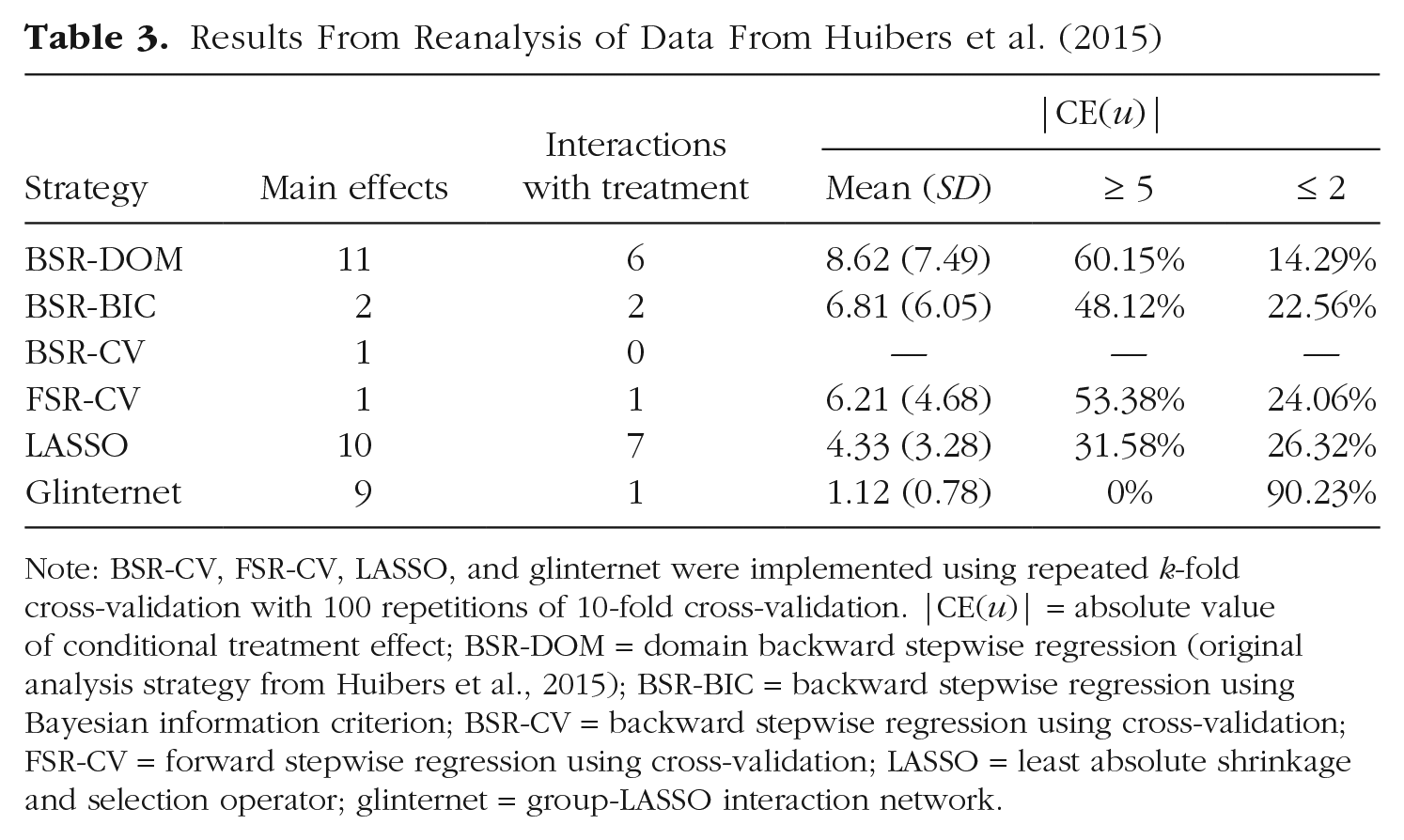
Note: BSR-CV, FSR-CV, LASSO, and glinternet were implemented using repeated k-fold cross-validation with 100 repetitions of 10-fold cross-validation. |CE(u)| = absolute value of conditional treatment effect; BSR-DOM = domain backward stepwise regression (original analysis strategy from Huibers et al., 2015); BSR-BIC = backward stepwise regression using Bayesian information criterion; BSR-CV = backward stepwise regression using cross-validation; FSR-CV = forward stepwise regression using cross-validation; LASSO = least absolute shrinkage and selection operator; glinternet = group-LASSO interaction network.

In total, nine different treatment-covariate interactions were included, taking all strategies together. There was some overlap between models concerning these interactions (see Table 4). Four treatment-covariate interactions were included in more than one model: attributional style–achievement (Attributional Style Questionnaire; Peterson et al., 1982; BSR-DOM, BSR-BIC, LASSO), interpersonal problems–self-sacrificing (Inventory of Interpersonal Problems; Horowitz et al., 1988; BSR-DOM, BSR-BIC, LASSO), number of life events in past year (BSR-DOM, BSR-BIC, LASSO, glinternet), and cognitive problems (Brief Symptom Inventory; Derogatis & Melisaratos, 1983; BSR-DOM, LASSO). By contrast, five treatment-covariate interactions were selected by only a single covariate-selection strategy. This highlights the uncertainty that is associated with interpreting results concerning prescriptive factors in this research setting (i.e., in a setting with a comparatively small sample size, many candidate variables, and correlations among these variables).

Table 4.

Moderators of Treatment Effect Selected by Different Covariate-Selection Strategies

Moderator	Method
	BSR-DOM	BSR-BIC	BSR-CV	FSR-CV	LASSO	glinternet
Number of life events in past year	X			X	X	X
Achievement (ASQ)	X	X			X
Self-sacrificing (IIP)	X	X			X
Cognitive problems (BSI)	X				X
Somatic complaints (BSI)	X
Paranoid symptoms (BSI)	X
Cold/distant (IIP)					X
Cognitive reactivity – acceptance (LEIDS)					X
Number of life events in life					X

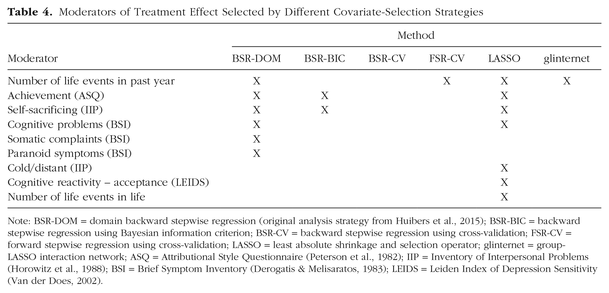
Note: BSR-DOM = domain backward stepwise regression (original analysis strategy from Huibers et al., 2015); BSR-BIC = backward stepwise regression using Bayesian information criterion; BSR-CV = backward stepwise regression using cross-validation; FSR-CV = forward stepwise regression using cross-validation; LASSO = least absolute shrinkage and selection operator; glinternet = group-LASSO interaction network; ASQ = Attributional Style Questionnaire (Peterson et al., 1982); IIP = Inventory of Interpersonal Problems (Horowitz et al., 1988); BSI = Brief Symptom Inventory (Derogatis & Melisaratos, 1983); LEIDS = Leiden Index of Depression Sensitivity (Van der Does, 2002).

All alternative models led to smaller mean absolute conditional treatment effects than BSR-DOM. BSR-BIC, FSR-CV, and glinternet can be explained by the fewer interactions included. For LASSO and glinternet, the shrinkage of coefficient estimates should be the reason for the smaller mean compared with BSR-DOM.

Discussion

In this study, we aimed at comparing six covariate-selection strategies in their utility for estimating ITEs in psychotherapy research. We conducted a Monte Carlo simulation that comprised 72 conditions mimicking typical settings of psychotherapy research. Those conditions varied along several factors known or hypothesized to influence the performance of covariate-selection strategies.

Across the 72 conditions studied here, shrinkage methods showed the best overall performance: LASSO and glinternet combined led to the most accurate out-of-sample predictions, identified the most true treatment-covariate interactions, and estimated most precisely true ITEs in the largest number of conditions. But pertaining to the inclusion of false positive treatment-covariate interactions and estimating the variance of ITEs, other strategies performed better in most conditions. Therefore, a first conclusion we draw from this study is that the best choice among the six covariate-selection strategies depends on the aim of the analysis: If the goal is to estimate ITEs, LASSO and glinternet can be a good choice, but if researchers want to estimate the variance of ITEs, stepwise-regression procedures perform better. Although detecting prescriptive factors and estimating ITEs is of utmost importance for the practical implementation of personalized treatment selection, estimating the variance of ITEs is of interest to assess the overall benefit one might expect from such an implementation (with a higher variance indicating greater potential benefit).

In addition, even if researchers were solely interested in one of the selection criteria studied here, results of this study do not give reasons to generally recommend usage of one strategy when choosing from the five strategies considered here. Especially sample size and SNR showed remarkable interactions with covariate-selection strategy for many evaluation criteria, but also, correlation among predictors, the number of irrelevant covariates, and (to some extent) hierarchy influenced the performance of covariate-selection strategies. Depending on the combination of these factors, different strategies might lead to the most favorable results. BSR-BIC, for example, showed a detrimental performance in small sample sizes but was a serious competitor for larger sample sizes (N ≥ 150). Whereas in some conditions, differences to other selection strategies seem marginal, for others, choosing LASSO over another strategy would bear a clear advantage. For example, in the case of a sample size of 600, a low SNR, correlation among predictors, 60 irrelevant covariates, and strong hierarchy, LASSO and glinternet identified all six treatment-covariate interactions in more than 70% of all simulation iterations. In contrast, BSR-DOM identified all relevant moderators in only 2.1%, and FSR-CV and BSR-CV identified all moderators in less than 1% of all iterations for this condition. However, in this condition, LASSO included at least 8.2 irrelevant treatment-covariate interactions in 50% of all iterations, whereas BSR-DOM included at least 4.6, glinternet included at least 3.6, and FSR-CV and BSR-CV included no false moderators in 50% of all iterations. This also illustrates why LASSO is classified as a variable screener. LASSO casts a wider net, so to speak, catching a lot of garbage but all fish as well. Although other methods might tend to catch only fish (finding the exact model) more often, LASSO produces a model that includes all relevant variables in many instances.

In particular, the present results are consistent with Hastie et al.’s (2017) findings that BSR and FSR using cross-validation can perform better than LASSO in conditions characterized by a higher SNR. Whereas Hastie et al. mainly evaluated performance with respect to out-of-sample predictions, this study showed that the possible advantage of BSR-CV and FSR-CV in high SNR conditions also applies to estimating ITEs. Furthermore, an advantage of glinternet over other strategies, particularly LASSO, as another shrinkage method was observed in some conditions, which were characterized by a strong hierarchy. This shows that the additional restrictions introduced by glinternet can enhance out-of-sample predictions and estimation of conditional treatment effects when these constraints conform to properties of the problem setting. Weak hierarchy in the true model, on the other hand, does not seem to deteriorate performance of glinternet substantially.

Moving from a comparative to an absolute evaluation of covariate-selection strategies in this study, one should take into consideration the rather wide distributions of some evaluation criteria, specifically in smaller sample sizes. Concerning the identification of treatment-covariate interactions, LASSO, for example, had a median TPR_IA of about .50 in conditions characterized by a sample size of 150 and a low SNR—the best result in comparison with other strategies. Yet the distribution ranged from 0 to 1 across these conditions so that in some replications of the simulation, none or all interaction effects were identified. This underlines the requirements concerning the sample size that have to be met if researchers want to avoid a high degree of uncertainty when analyzing heterogeneity of treatment effects. Similar to results from Luedtke et al. (2019), in our simulation, distributions for TPR_IA became sufficiently narrow for iterations with a sample size of 300 in each treatment condition. These findings stand in contrast to sample sizes in RCTs on personalized treatment selection and might explain the lack of consistent results pertaining to prescriptive factors (Lorenzo-Luaces et al., 2021).

Moreover, the reanalysis of data from an empirical study on PAIs of CT and IPT (Huibers et al., 2015) highlighted the consequences of selecting a covariate-selection strategy in a real-world setting. Looking at the percentage of absolute PAIs greater than 5 (a BDI difference deemed clinically significant), one would come to quite different conclusions about the impact of allocating patients to their optimal treatment on the basis of different covariate-selection strategies. Using the original selection strategy (BSR-DOM), we would assume that more than half the patients would (in the clinical sense) significantly profit from allocation to their optimal treatment, whereas according to LASSO, we would assume that this is the case for less than a third of all patients. The same holds for the inclusion of treatment-covariate interactions: Both strategies disagreed in five moderators that were included in the respective final models. Looking at Figures 1 and 3, one might assume that LASSO would serve better than BSR-DOM as a variable screener for treatment-covariate interactions and for estimating ITEs in a scenario with this sample size. Median TPR_IA and median $\mathrm{RMSE}\left(\widehat{\delta }\right(u))$ were also higher for LASSO than for BSR-DOM in the case of correlation among predictors and a larger number of candidate variables (as is the case in the data set). But because of the wide distributions, there is some level of uncertainty associated with this assumption.

Limitations and future directions

The first question that arises concerning the results from this study is whether they apply to the analysis of nonsynthetic data: How “realistic” is the simulation study, especially concerning data generation, and what can we conclude for the analysis of RCTs? We put a lot of effort into mimicking the challenges of psychotherapy research; however, our study cannot completely account for the complexity of empirical data (e.g., multivariate nonnormal distributions). For example, several variables in the data provided by Huibers et al. (2015) exhibited a considerable amount of skewness. In addition, in our simulation design, correlations among predictors pertained only to relevant predictors, whose true coefficients were not zero. Thereby, our simulation design fulfilled the “irrepresentable condition” for model selection consistency of LASSO, which potentially gives LASSO an advantage (Zhao & Yu, 2006). In contrast, it is possible that researchers will include two (or more) correlated variables in their investigation of which only one (or a larger subset) is truly associated with outcome. Only low-order interactions and linear relationships have been modeled in this study, thereby creating an optimal setting for the selection strategies investigated here. Our study gives an orientation when each strategy might be best applied and highlights the importance of investigating the effects of different factors (e.g., SNR) on the performance of covariate-selection strategies.

Furthermore, this study examined only two of several possible criteria to evaluate the consequences of choosing a covariate-selection strategy on estimating ITEs. Foremost, this study looked at estimating ITEs (through conditional treatment effects) for the same sample that the model was built on. By this means, we followed the analysis strategy of existing empirical trials (e.g., Deisenhofer et al., 2018; Huibers et al., 2015). Future investigations may also examine the accuracy of out-of-sample predictions of ITEs, an important factor for the practical implementation of results from a study on heterogeneous treatment effects (e.g., Lutz et al., 2019; Schwartz et al., 2021; van Bronswijk, Bruijniks, et al., 2021). Likewise, we evaluated only the inclusion of true and false treatment-covariate interactions. However, in empirical trials, researchers usually do not solely look at whether effects are included but interpret effect sizes. Especially for shrinkage methods (i.e., LASSO, glinternet), it might be the case that included false treatment-covariate interactions tend to be of negligible size.

Because the number of covariate-selection strategies that we investigated was limited, future studies may examine further methods in their utility for estimating ITEs. These include methods suited for more complex relationships among variables (e.g., random forests; Breiman, 2001), methods explicitly developed to account for hierarchy constraints when identifying interactions, (e.g., Sail, Bhatnagar et al., 2020; VANISH, Radchenko & James, 2010; or Dirichlet process, forests, Du & Linero, 2019), and other methods suited for n $\mathrm{<}\mathrm{<}$ p scenarios (e.g., as investigated by Ternès et al., 2017). Furthermore, in this study, model selection was based on outcome prediction accuracy. Rolling and Yang (2014) showed that model selection based on minimizing the expected prediction risk (indirectly through information criteria such as BIC or directly through cross-validation) does not necessarily lead to the model that best predicts conditional treatment effects or reflects the heterogeneity of treatment effects (also see Powers et al., 2018). Several metrics for model selection in the context of predicting conditional treatment effects have been developed in recent years (Schuler et al., 2018). Future studies may evaluate their use in psychotherapy research.

Concerning the strategies using cross-validation, a major problem of 10-fold cross-validation became apparent in the reanalysis of data from Huibers et al. (2015): 10-fold cross-validation is susceptible to instability in small sample sizes. Randomly splitting the data into folds introduces additional variability, which means in the case of covariate selection, different covariates are included in the final model depending on how the data are split. This does not apply to “exhaustive” splitting schemes, such as leave-one-out cross-validation, because they do not include randomness in data partitioning. In summary, as with other rules-of-thumb, the question of which cross-validation approach to use is much more complicated than general recommendations suggest. Especially for small sample sizes, we advise against using simple k-fold cross-validation. By using repeated 10-fold cross-validation in the reanalysis of data from Huibers et al. (2015), we reduced the comparability with our simulation analysis but used an approach that was more suitable to the problem setting at hand.

Our study mainly focused on identifying treatment-covariate interactions and estimating ITEs. However, for the purpose of building a decision rule for allocating patients to their optimal treatment, it is important to evaluate the benefit of such an allocation (e.g., compared with a random allocation). To this end, several estimators have been developed (Sies & Mechelen, 2019) and call for evaluation within the frame of psychotherapy research.

Conclusion

Analyzing ITEs is of utmost importance for the advancement of personalized medicine, which enables the allocation of patients to their optimal treatment. This is important not only from a patient’s point of view but also for the organization of cost-effective health-care systems by making optimal use of limited resources. Misestimating ITEs, on the other hand, can have negative ramifications by leading to allocating patients not to their best treatment option—and in the worst case, to a harmful treatment for particular patients.

On the basis of our simulation, we make the following recommendations for future studies on personalized treatment selection in psychotherapy: When estimating ITEs, researchers may consider covariate-selection strategies from different method “families,” such as shrinkage methods or stepwise regression, because each method is best suited for specific problem settings. We recommend that these methods are evaluated regarding the factors investigated in this study. Some of these factors can be determined (e.g., the sample size), others need to be estimated (e.g., the covariance structure), and yet for others, researchers have to propose assumptions (e.g., the number of relevant treatment-covariate interactions). If the sample to be analyzed is rather small, researchers may try to conduct small simulation studies themselves that closely resemble their problem setting, thereby making an informed choice on the covariate-selection strategy. R-package SimDesign (Chalmers, 2020) provides a framework easy to use for simulation studies that does not require a strong background in programming. Researchers may use the script we published at OSF (https://osf.io/u24en) as a starting point. However, if the sample size is large enough, we recommend that researchers apply several methods and select the best one by using a two-step approach: First, the data are split into a train-test set and a holdout set. For each method, the best model is selected by making use of the train-test set (e.g., through [repeated] k-fold cross-validation). The performance of the final models from each method is then compared by making predictions for the holdout set (for a practical application of this approach, see Webb et al., 2020). In any case, researchers are encouraged to explain how they came to conclude that the covariate-selection strategy they finally selected was the best choice for the specific problem at hand.

Supplemental Material

sj-html-2-cpx-10.1177_21677026211071043 – Supplemental material for Covariate Selection for Estimating Individual Treatment Effects in Psychotherapy Research: A Simulation Study and Empirical Example

Supplemental material, sj-html-2-cpx-10.1177_21677026211071043 for Covariate Selection for Estimating Individual Treatment Effects in Psychotherapy Research: A Simulation Study and Empirical Example by Robin Anno Wester, Julian Rubel and Axel Mayer in Clinical Psychological Science

Supplemental Material

sj-pdf-1-cpx-10.1177_21677026211071043 – Supplemental material for Covariate Selection for Estimating Individual Treatment Effects in Psychotherapy Research: A Simulation Study and Empirical Example

Supplemental material, sj-pdf-1-cpx-10.1177_21677026211071043 for Covariate Selection for Estimating Individual Treatment Effects in Psychotherapy Research: A Simulation Study and Empirical Example by Robin Anno Wester, Julian Rubel and Axel Mayer in Clinical Psychological Science