Sage Journals: Discover world-class research

Abstract

In developing countries, such as India, the seasonal nature of agriculture becomes a primary cause of economic distress. In response, households engage in migration as a coping mechanism to diversify the risk as well as for maximising household income during agricultural slack season. Thus, households collectively decide to send one or more members away with the assurance that the migrant will send a part of their urban income, enabling the household to improve living standards through increased consumption expenditures. In this light, this study focuses on seasonal out-migration from the states of Bihar, Jharkhand and Orissa in India. Using the International Crop Research Institute for the Semi-Arid Tropics East-India panel data set for 2011–2014, the study attempts to analyse the determinants of intensity of migration for the panel data. Second, we try to evaluate the impact of migration on the consumption expenditure of left-behind households using inverse probability-weighted regression. The analysis of the determinants of migration suggests the presence of distress migration where external shocks in the form of climate change-related losses increase the migration intensity of the households, highlighting migration as a coping mechanism. The second part of the study reveals higher per-capita food as well as non-food expenditure for the migrant households as compared to the non-migrants based on the yearly cross-section analysis. These findings suggest the positive effects of seasonal migration on left-behind families.

Keywords

Internal labour migration left-behind families panel data treatment effects East India

Introduction

Developing countries often experience patterns of unequal economic growth, with a few regions growing more than others. Such regional inequalities in growth then transform into inequalities in income and opportunities. Individuals and households engage in inter-regional migration to seek advantage of better opportunities in urban economic centres (Ravenstein, 1885), making migration an inevitable consequence of economic development. Additionally, in agrarian economies like rural India, where weather-dependent and volatile agricultural income is the primary source of livelihood, push factors from rural areas become the dominant force in determining migration. This type of migration is often seasonal in nature and is undertaken in accordance with the crop cycle. Here, the role of government becomes crucial to generate employment opportunities during the slack season and to provide affordable insurance and credit to rural households. In the last two decades, the Indian government has initiated various schemes to provide employment and credit in rural areas, such as the Mahatma Gandhi National Rural Employment Guarantee Act and the Kisan Credit Card scheme. Such government initiatives reduce the dependence on seasonal migration.

Most studies highlight that seasonal migration takes place under unfavourable economic and social circumstances, with the households belonging to lower social strata, having higher borrowings, lower landholdings and lower farm incomes participating in seasonal migration more often (Deshingkar & Start, 2003; Keshri & Bhagat, 2012; Marta et al., 2020; Nienkerke et al., 2023; Pradhan & Narayan, 2020). Additionally, the weather dependency of agriculture makes it more susceptible to sudden climatic changes and, thus, impacting rural livelihood. There are prominent interlinkages between climate change and rural-to-urban migration as climate change increases the vulnerability through loss of livelihood for the rural household (Choksi et al., 2021; Pradhan & Narayanan, 2019, 2020). These unforeseen climatic changes often increase the volume as well as the intensity of migration from rural to urban areas. Such a form of migration is often referred to as ‘distress migration’ (Deshingkar, 2017). In response, the household collectively decides to send one or more household members to urban areas to expand their income portfolios and deal with economic distress (Stark & Bloom, 1985; Stark & Lehvari, 1982).

Additionally, given the predominantly seasonal pattern of agriculture in rural India, seasonal migration assumes a crucial role in increasing the resources of left-behind families through contribution to family income. This is often observed through improved household consumption expenditures and, thus, improving their daily livelihoods. In this sense, migration helps the entire household to achieve a better standard of living (Démurger & Wang, 2016). How the increased income is perceived and spent differs across households and can have varied implications for the well-being and improved livelihoods of the left-behinds (Adams & Cuecuecha, 2010; Castaldo & Reilly, 2007; Clément, 2011; Démurger & Wang, 2016; Randazzo & Piracha, 2019; Wang et al., 2021).

Given this background, the study contributes to the discussion in the following two ways. First, we ask whether the rural households from eastern India are dependent on migration as a risk-diversification strategy even in the presence of government schemes and what are the determinants of the intensity of migration. The findings show that the government support does not reduce the intensity of seasonal migration and the climatic shock remains the major determinant of migration. Second, we estimate the impact of the intensity of seasonal migration on the consumption expenditure of families. The findings reveal a positive impact of migration as left-behind families experience higher per-capita food as well as non-food expenditure. For this study, we use panel data for 2011–2014 from the International Crop Research Institute for the Semi-Arid Tropics (ICRISAT), which collects household-level information from East Indian villages.

The remaining paper is divided into the following sections: the second section provides conceptual background. The third section discusses the data sources, the description of selected variables and the results for descriptive analysis; the fourth section describes the econometric methodology followed for the study; the fifth section discusses the empirical findings; and lastly, the sixth section presents the conclusion of the study.

Conceptual Background

The present study examines the determinants of the intensity of seasonal migration at the household level. Second, it attempts to estimate the effect of seasonal migration on household consumption expenditure. This work is based on two strands of literature. The first strand, referred to as the ‘new economics of labour migration’ (NELM), views migration as the collective decision of the household rather than an individual decision. NELM provides motivations behind sending migrants from the household. The second strand talks about the effect of migration on the families at the origin. Migration may affect various aspects of the families at the origin, such as consumption, investment opportunities, child development and women empowerment. We focus on the effect of seasonal migration on the consumption expenditure of the families. We elaborate below on these two strands and discuss the contribution of the present study to the literature.

Seasonal migration is generally adopted in rural India to tap the income-generating avenues during the agricultural slack season. Under this scenario, a few members of the farmer household migrate to urban and semi-urban areas to find temporary jobs and to support the family during the slack season (Deshingkar & Start, 2003; Haberfeld et al., 1999). Thus, the decision to migrate is usually a collective decision at the household level. These motives behind the seasonal migration are theoretically modelled by Stark and Bloom (1985) and Stark and Lucas (1988). The conceptual framework given in these papers works as the foundation for the empirical literature on motives behind migration. This framework is widely known as the theory of NELM. Here, the household and the migrant enter a self-enforced contract, ensuring a continued transfer of income from the migrant to the left-behind families (Stark & Bloom, 1985; Stark & Lucas, 1988). Mincer (1978) also argues that the net family gains rather than the net personal gains motivate the household to engage in migration. Thus, the household becomes the decision-making unit in rural agricultural settings, adopting seasonal migration as a livelihood strategy.

As the household engages in seasonal migration, migration patterns highlight different motives under which the decision is usually taken. There are two primary motives for migration in lines with the NELM: risk diversification and investment.¹ Risk diversification can primarily be done through either maximising the income or through minimising the risk of loss of income stream due to unforeseen events as these are, in turn, the most relevant motives in case of seasonal migration (Marta et al., 2020; Stark & Levhari, 1982). When the household decides to send its members for migration during the slack season of agriculture, their motive is to increase the familial income. Here, migration becomes a livelihood strategy when the sources of employment are limited within the village. Thus, migrants move frequently for a shorter duration, with the intention to return during the peak season. Consequently, they get absorbed in low-paying informal jobs with wage rates even lower than what is prevailing in the rural sector. This is often known as distress-induced migration where migration takes place to support the survival of the poor household rather than a free choice (Dodd et al., 2016).

Additionally, migration is undertaken in order to diversify the risk, where households migrate to diversify their income streams in order to deal with any unforeseen events. Given the predominantly weather-dependent nature of agriculture in rural areas, the threat of adverse effects of climate change prevails. The loss of income from sudden changes in climate can be detrimental to the smooth consumption and survival of the households (Morten, 2019). Consequently, seasonal migration is perceived as an effective coping strategy for the household. This is more prominent in regions where there is a lack of formal credit and insurance markets, and thus, households self-insure by sending one or more members away (Stark & Levhari, 1982). Thus, the destination the household chooses for migration is such that the income opportunities are either statistically uncorrelated or negatively correlated with the earnings of the place of origin (Stark & Bloom, 1985). In this sense, migration with the motive of risk diversification not only provides insurance to the household in case of crop failure but at the same time, ensures a continued income source when fewer opportunities are available in the villages (Marta et al., 2020).

Now, as the household engages in migration, the question arises that how many members to send away for migration, that is, what the intensity of migration within the household should be. Rapoport and Docquier (2006) develop a formal model for determining the optimum migration rate within the household. The optimum level is likely to increase with the quantity and quality of familial land (referred to as technological parameter) but decreases with the cost of migration and the minimum level of subsistence for the household. They argue that the household is likely to keep sending migrants as long as the familial income keeps increasing to seek advantage of increased income transfers. However, the decision is constrained by the cost of undertaking migration for each member, limiting the intensity of migration. For each household, the optimal number of migrants and the number of migrants it can afford to send will be different. This is especially true for poorer households as they are faced with severe liquidity constraints.

Previous literature measures the intensity of migration at both macro- and micro-levels. At the macro-level, studies such as Keshri and Bhagat (2012) measured intensity as the rate of migration per 1,000 population at the district level. In the case of micro-level studies, the intensity of migration is calculated at a smaller unit, such as a household. Akhter and Bauer (2014) and Pradhan and Narayanan (2019) measure the intensity of migration at the household level, taking it as the proportion of migrants from the total members and working-age members in the household, respectively. In this study, we measure the intensity of migration by combining the volume as well as the frequency of migration using person-months as we account for the time spent outside the village, which captures the essence of seasonal migration. This is opposed to the other studies which majorly focus on the volume of migration only. Thus, using the above concepts, we analyse the determinants of the intensity of seasonal migration in the rural villages of East India.

Moreover, as in the NELM household finds motivation to engage in migration, it is crucial to understand the effect of seasonal migration in improving the overall living standards of the migrant household. One of the many ways of observing the improvement in living standards is through measuring the changes in the consumption expenditure of the household. With seasonal migration, migrating members of the household have a vested interest in the family due to frequent returns. Thus, they opt to maintain ties with the family at origin through private transfers (Lucas & Stark, 1985). These private transfers have the potential to impact not only household consumption but also have consequences on the economic development of the migrant-sending areas through productive investments (Démurger & Wang, 2016). However, based on household circumstances and structural conditions (social and economic), especially for poorer households, consumption rather than investment becomes a priority (Koc & Onan, 2004). At the microeconomic level, the increased income through undertaking migration has the potential to encourage better consumption, savings and investment in education and health of children, and thus, are crucial for improvement in the livelihood of the household (Clément, 2011).

Across the strand of literature dealing with migration and expenditure patterns, there are three popular views on how left-behind families perceive migrant incomes and how migration affects their expenditure patterns: first, the income is fungible and treated as any other income of the household and thus, at the margin, it is spent like any other income; second, it alters consumption behaviour of the migrant households and they spend most of their income on consumption rather than investment; and last, known as the more optimistic view which is based on the permanent income hypothesis where migrant income is treated as a transitory income, and thus, is spent at the margin towards more productive investment (Adams & Cuecuecha, 2010; Castaldo & Reilly, 2007; Clément, 2011; Démurger & Wang, 2016; Randazzo & Piracha, 2019; Wang et al., 2021; Yuni et al., 2018).

The empirical studies on the impact of migration on consumption expenditure are mixed. It is often argued that the impact depends on the nature of the jobs that migrants get in the urban area (Chandrasekhar et al., 2015). At the same time, the motives of the household behind undertaking migration become crucial in determining their consumption patterns (Chandrasekhar et al., 2015; Marta et al., 2020). While a large segment of literature finds that having a migrant in the household increases the consumption expenditure of left-behind families, various studies also show the impact on the consumption expenditure of left-behind families to be negative, with the increase in household income being diverted towards productive investments (Castaldo & Reilly, 2007; Chandrasekhar et al., 2015; Wang et al., 2021). Further, if the migrant is engaged in low-paying casual jobs, which is often the case in seasonal migration, the impact is insignificant in such cases. This is primarily because even if urbanisation means expanding economic opportunities in the cities, the nature of opportunities does not match the skill set of the individuals migrating from rural areas (Todaro, 1969). Additionally, the migration undertaken with the risk-diversification strategy may lead to an insignificant impact on the consumption of the household. In contrast, migration as an investment strategy is more likely to have a positive impact (Marta et al., 2020).

Moreover, many studies have observed a shift in the behavioural patterns where the migrant household’s consumption pattern may differ knowing there is a presence of migrants in the household (Castaldo & Reilly, 2007; Wang et al., 2021). Migrant households are likely to self-select themselves into migration, indicating the presence of selection bias in the data. The characteristics of households such as education, occupational status, attitude towards risk, size of the family, etc., which can cause differences in the decision to engage in migration are also likely to explain the differences in the expenditure patterns of the households after increased income due to migration. We, therefore, use the inverse probability-weighted (IPW) regression using propensity score as weights to eliminate the selection bias (Antman, 2013; Caliendo & Kopeinig, 2008; Kuhn et al., 2011; McKenzie et al., 2010).

In light of the above discussion, the aim is to understand, first, the determinants of the intensity of seasonal migration; and second, to understand the impact of migration on the per-capita consumption expenditure of the left-behind families of the migrants. This is estimated for per-capita food and non-food expenditure using panel data for eastern India as well as year-wise cross-sections.

Data and Variables

The study uses household-level panel data from the ICRISAT for Bihar, Jharkhand and Orissa for the period 2011–2014.² These three states in the eastern part of India are densely populated, with large proportions of the population living below the poverty line (Datta, 2020; Economic Survey of India, 2022). The data is collected from 12 villages using multiple schedules which cover a wide range of individual, household and village-level variables describing the demographic, social, economic and climatic conditions. The information on migration is available in the employment schedule, which collects monthly data. Table 1 describes the outcome variables, that is, food and non-food consumption, the treatment variables, that is, migration status and intensity, and other control variables.

Table 1.

Description of Variables Used in the Study for the Household Level Analysis.^a

Variable	Description
Outcome variables^b
Food expenditure	Per-capita annual food expenditure aggregated at the household level
Non-food expenditure	Per-capita annual non-food expenditure aggregated at the household level
Treatment variables
Migration status of the household	1 = a household consisting of one or more migrant members (who are 15–59 years of age and migrated for two or more months in a year) is taken as a migrant household; 0 = otherwise
Intensity of migration	Proportion of the number of person-months used for migration in a household to the total number of person-months available in a household^c
Other controls
Economic indicators
Wage differential	One-period lag of the difference between the average urban wage and the average rural wage rate taken at the village level^d
Borrowings	Borrowings as a proportion of the real consumption expenditure of the household^e
Operational landholdings	Log of land used by the household for producing agricultural output (in ac)
Asset index^f	Household asset index created based on the ownership of 27 consumer durables
Farming household	1 = household is deriving their income from farming as their main occupation; 0 = otherwise
Benefit received from government developmental scheme	Benefits received in monetary terms from participating in government developmental schemes related to employment only
Annual rainfall	One-period lag of the amount of rainfall received in the village
Loss from adverse climatic events	Loss in rupees experienced due to adverse climatic events occurred in the previous year
Demographic indicators
Level of education in a household	The maximum level of education achieved by any working age member in a household: 0 = no education; 1 = till primary; 2 = till senior secondary; 3 = till higher secondary; 4 = graduate and above
Size of the family	Total number of members in a household
Working members	Total number of working age members in a household (15–59 years of age)
Social indicators
Caste group	1 = Forward caste; 2 = other backward castes (OBC);^g 3 = Scheduled Castes and Scheduled Tribes (SC and ST)
Religion	1 = Hindu; 2 = non-Hindu

Source: ICRISAT East-India data set (2011–2014).

Notes: ^aAll monetary variables are in per-capita and real terms and have been adjusted using a price index taking 2011–2012 prices as the base. Further, all these variables are presented in log form (except wage differential).

^bThe per-capita quantities in outcome variables are obtained by dividing the annual expenditures with the number of non-migrating members of the household. Migrating members of the household have been removed as approximately 60% of the migrants are migrating for at least nine months in each year.

^cThe total number of person-months have been calculated by multiplying the total number of working-age family members in a household by the number of months in a year. Further, the total number of months where each migrant has migrated has been aggregated at the household level.

^dRural wage rates are calculated at the village level for the farm activities for current year. On the other hand, migrant’s wages are taken to represent the urban wages. Wage differential has been lagged by one year as expected average wage differential of the previous period determines the migration in the current year.

^eBoth borrowings and consumption expenditure are lagged by one period as the financial burden of the previous period determines the migration behaviour in the current period.

^fAsset index was created using the principal component analysis (PCA) using the methodology of Filmer and Pritchett (2001) based on the ownership of 27 consumer durables for each household. Based on the asset score from conducting PCA, the households were divided into three categories (poorest 20%, middle 60% and richest 20%) for each of the three states.

^gOther backward caste includes backward caste (BC) and special backward caste (SBC)/socially and economically backward caste (SEBC)/extremely backward caste (EBC).

In each year, the data is collected from 470, 484, 492 and 497 households, respectively, from the three states. The panel is unbalanced as when a household is divided, the spin-off households are also included in the survey with new heads of the household. In the overall sample, the proportion of migrant household ranges from 0.28 to 0.33 over the study period (Table 2). The intensity of seasonal migration, defined in terms of person-months, differs marginally across all four years of study and lies in the range of 0.24 to 0.27 (Table 2). Also, around 60% of the households in each year derive their income from farming activities except for 2014, where the majority of the households are deriving their income from non-farming activities. The most favourable destination for out-migration in this sample is Delhi, receiving nearly 14–20% of total migrants every year. This is followed by Maharashtra with 10–14% and Kolkata with 2–5% of the total migrants. Such a pattern shows the preference of the migrants towards metropolitan cities with greater employment opportunities.

Table 2.

Summary of Treatment Variables Across Years (in Percentage).

Treatment Variable	2011	2012	2013	2014
Percentage of migrant households	32.42	30.79	28.46	28.08
Intensity of migration	26.83	26.34	24.05	26.21

Source: Calculated using ICRISAT East-India data set (2011–2014).

In this study, as we analyse the impact of migration on the outcome variables, per-capita food as well as non-food expenditures, we expect migration to improve the consumption expenditure of the left-behind families. Comparing their mean expenditures, we find that the per-capita food expenditure is higher for the migrant households than the non-migrants for all years except 2014. Similarly, the per-capita non-food expenditure is higher for the migrant households as compared to the non-migrants for all years except 2012 (Table 3). This preliminary analysis indicates an overall higher consumption expenditure for the left-behind families of the migrant households. However, the further possibility of selection bias and its impact on the difference in consumption pattern among migrant and non-migrant households is explored in the empirical analysis.

Table 3.

Descriptive Statistics for the Year 2011–2014.^a

Variables	Year
	2011		2012		2013		2014
	Migrant N = 154	Non-migrant N = 316	Migrant N = 149	Non-migrant N = 335	Migrant N = 140	Non-migrant N = 352	Migrant N = 139	Non-migrant N = 356
Outcome variables
Food expenditure (₹)	7,307.66	6,403.79	5,765.42	4,904.20	5,944.24	5,648.89	6,559.51	7,006.68
Non-food expenditure (₹)	6,874.97	5,693.56	9,028.10	10,845.27	3,420.60	2,944.69	5,384.90	5,017.36
Economic indicator
Household borrowings (₹)	2,262.47	1,985.16	4,670.04	3,579.67	5,922.06	3,298.88	4,849.56	6,958.88
Operational landholdings (ac)	2.07	2.25	2.06	2.18	2.09	2.23	2.08	2.18
Benefit from government scheme (₹)	756.59	656.51	145.21	275.33	100.27	189.91	352.66	801.37
Loss due to adverse events (₹)^b	2,239.51	2,675.30	1,558.26	2,375.97	2,239.84	2,678.66	1,753.21	2,327.69
Demographic indicator
Size of the family	7.36	5.41	7.54	5.42	7.36	5.25	7.26	5.23
Average years of schooling	6.46	5.65	6.75	5.78	7.27	5.84	7.10	6.06
Social indicators
Religion
Hindu	33.02	66.98	30.80	69.20	28.31	71.69	28.48	71.52
Non-Hindu	30.43	69.57	30.61	69.39	29.79	70.21	25.53	74.47
Caste
Forward caste	41.44	58.56	37.39	62.61	36.61	66.39	31.40	68.60
OBC	35.63	64.37	32.84	67.16	29.09	70.91	34.80	65.20
SC and ST	15.31	84.69	17.82	82.18	18.10	81.90	17.16	82.84

Source: Calculated using ICRISAT East-India data set (2011–2014).

Notes: ^aAll monetary variables are taken in per-capita and real values in order to standardise the variables making the households comparable.

^bThe number of households that recorded loss from adverse climatic events is lesser than the total number of migrant and non-migrant households. In each year beginning from 2011, 75, 51, 32 and 38 migrant households suffered climatic loss, respectively. Similarly, 147, 101, 58 and 51 non-migrant households suffered climatic loss in each year, respectively.

Economic Indicators

The operational landholdings of the households are lower for the migrant households as compared to the non-migrant households. These observations indicate the role of seasonal migration as a source of additional income. Lower operational landholdings also represent weaker ties to the villages, encouraging more and more household members to migrate. Additionally, the benefits received from government schemes are lower for migrant households as compared to the non-migrants in each year except 2011, indicating insufficiency of the aid provided by the government. Additionally, the per-capita borrowings of the households are observed to be higher for the migrant households as compared to the non-migrant households except for in 2014 (Table 3).

As agriculture is primarily weather dependent in India with rain-fed cultivation, any unpredicted variation in weather conditions becomes a cause for uncertainty of income in rural households. This uncertainty increases the likelihood of migration to cope with the risk of varying incomes (Stark & Bloom, 1985). The data set provides information on the amount of loss caused due to adverse climatic events. We consider per-capita loss at the household level which is lower for the migrant households as compared to the non-migrants in each year.

Demographic Indicators

It is observed that for all four years, the size of the family is larger for the migrant households as compared to the non-migrant households conforming to the argument that larger family sizes increase the likelihood of migration. Similarly, the average years of schooling for migrant households are higher than the non-migrant households (Table 3). This result is supported by previous literature where it is seen that more educated individuals or households have a higher probability of engaging in migration (Bhagat, 2010; Zhu, 2002).

Social Background

We include two variables, religion and caste, to control for the social background of the households. Approximately, 28–33% of the Hindu households engage in migration while 25–30% non-Hindu households participate in migration over the period of study. Among the caste categories, Forward caste households display the highest proportion of households engaging in migration ranging from 31% to 41% as compared to the other two categories over the period of study (Table 3).

Econometric Methodology

The unit of analysis for the study is at the household level, where households are categorised as either migrant or non-migrant households. The analysis is conducted in two parts where first, we estimate the determinants for the intensity of migration, and then, estimate the impact of migration on the consumption of left-behind families.

Determinants of Intensity of Seasonal Migration

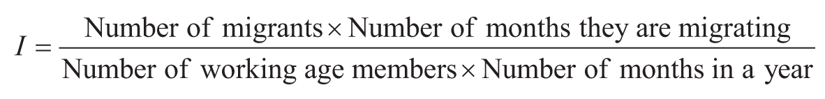
The intensity of seasonal migration (I) is defined in terms of the proportion of the number of person-months used for migration in a household to the total number of person-months available in a household. It is calculated as follows:

I = \frac{Number of migrants \times Number of months they are migrating}{Number of working age members \times Number of months in a year}

Here, the intensity of migration is a fractional response variable. Further, by definition, the intensity of migration lies in the range of [0,1] and thus, is a bounded fraction. In such cases, linear regression models will not give consistent estimates as the predicted probability might lie outside the unit interval. Papke and Wooldridge (2008) show how to specify and estimate a fractional response model (FRM) for the case of panel data with a large cross-sectional dimension and relatively fewer time periods. We use this model to estimate the intensity of seasonal migration in this study.

Let I_it represent intensity of migration across households i and time periods t. For the set of explanatory variables, the model assumes the following functional form:

E (I_{i t} | X_{i t}, c_{i}) = Φ (X_{i t} β + c_{i}); t = 1, \dots, T

(1)

where Φ(.) is the cumulative distribution function (CDF), c_i are the unobserved time-invariant effects which appear additively inside the CDF. For the dependent variable, since there are a large number of values observed at the endpoints, it follows the logistic distribution. Thus, with the generalised estimating equations approach, we will use the logit model as the link function for the panel data following the Bernoulli distribution. The explanatory variables are given by X_it which is a 1×k vector for any k variables.

Migration and Household Consumption Expenditure

Analysing the impact of migration on consumption expenditure gives rise to the issue of selection bias. Selection bias may arise due to differences in various observed and unobserved characteristics of migrant and non-migrant households. The factors such as the maximum level of education in the household, occupational status, size of the family, past migration from within the household and the household’s attitude towards risk are some of the major characteristics which may give rise to selection bias in the decision to migrate (Clément, 2011). Consequently, these factors may also cause change in the behavioural pattern of the household, thus influencing their expenditure patterns (Jimenez-Soto & Brown, 2012). It is, therefore, essential to eliminate the selection bias in order to get the true effect of migration on consumption expenditure of the left-behind families. We, thus, use IPW regression using propensity scores as weights to understand the effect of migration on the consumption expenditure of left-behind families. We do this with the cross-sectional data for each of the three years removing the selection bias due to observed characteristics. Also, to deal with selection bias arising due to unobserved characteristics of the household, we use the fixed effects method along with the IPW regression for the panel data of 2011–2014.

To remove the selection bias due to the observed characteristics,³ we estimate the propensity score P(X)⁴ taking the decision to migrate as the treatment variable. The results for the first-stage logit model estimating the propensity score are presented in Table A2. In this analysis, the treatment group gets weight equal to 1, while the control group is given weight equal to P(X)/1 − P(X). We use the IPW regression with ATT weights to estimate the effect of the household’s decision to engage in migration on the food and non-food expenditure of the left-behind families for each cross-section.

Second, we use IPW panel regression to estimate the effect of migration intensity on the per-capita food and non-food expenditure of the left-behind families. In order to account for selection bias due to the unobservable characteristics, we use the fixed effect estimation along IPW regression (Antman, 2013; Kuhn et al., 2011; Piracha & Saraogi, 2017). Here, we use the propensity scores for the year 2012, as for most of the households, the migration status does not change during the three years, to remove the selection bias. These propensity scores are then used as the IPWs (ATT) in the fixed effects model. Thus, we estimate the following equations along with IPWs (ATT):

F_{it} = α + γ_{i} + λ_{t} + δ I_{i t} + X'_{i t} β + ε_{i t}

(2)

{NF}_{it} = ω + γ_{i} + λ_{t} + ρ I_{i t} + X'_{i t} θ + μ_{i t}

(3)

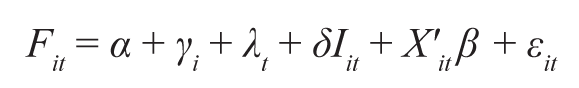
where F_it is the per-capita food expenditure of the ith household at time period t and NF_it is the per-capita non-food expenditure of the ith household at time period t. I_t is the intensity of migration calculated in person-months for the household. γ_i are the household fixed effects, λ_t is the time-fixed effects, X'_it is the vector of all the observed time-varying covariates.

Additionally, to check for the robustness of results for the panel analysis, we try to estimate the effect of intensity of migration on consumption expenditures by taking the average values of the explanatory variables from 2012 to 2014 while estimating the propensity scores. Here, we take the treatment variable, that is, the migration status of the household as 1 if a household has been classified as a migrant household at least once during the period of study and 0 otherwise.

Empirical Results and Discussion

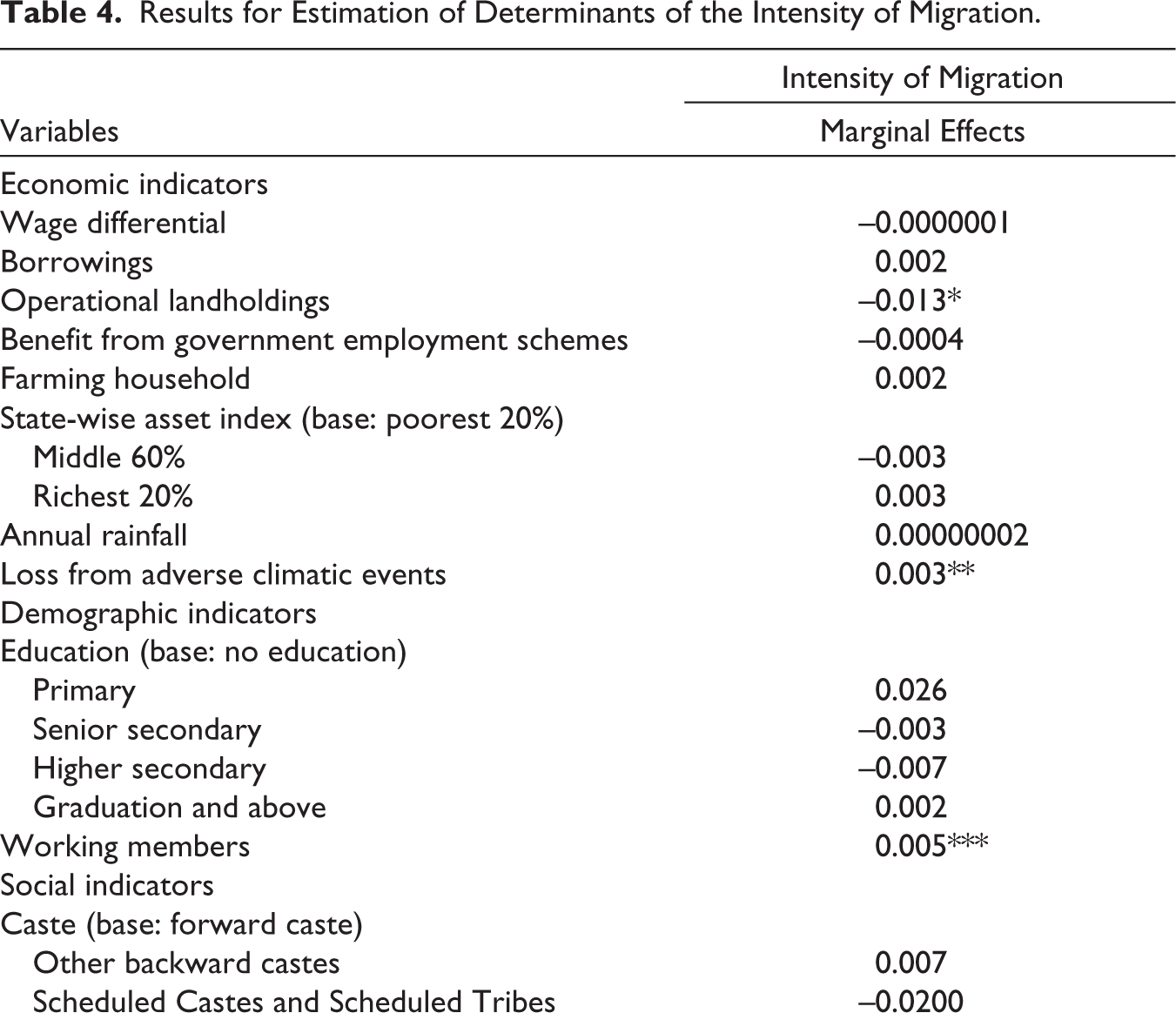
The empirical findings indicate the presence of distress migration in the rural parts of Bihar, Jharkhand and Orissa. We find a positive association between a family’s financial burden due to climatic losses and the intensity of seasonal migration (Table 4). Additionally, the analysis of the impact of migration on consumption expenditure reveals a positive impact on the left-behind families through increased per-capita food as well as non-food expenditure indicating improvement in livelihoods (Table 5).

Table 4.

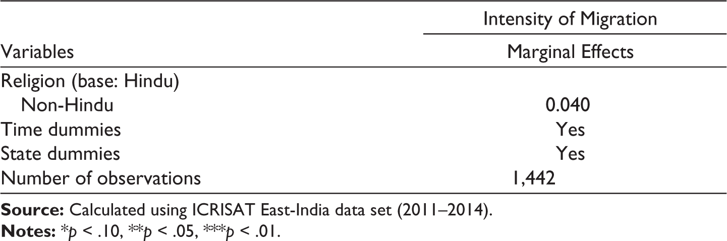
Results for Estimation of Determinants of the Intensity of Migration.

Variables	Intensity of Migration
Variables	Marginal Effects
Economic indicators
Wage differential	–0.0000001
Borrowings	0.002
Operational landholdings	–0.013*
Benefit from government employment schemes	–0.0004
Farming household	0.002
State-wise asset index (base: poorest 20%)
Middle 60%	–0.003
Richest 20%	0.003
Annual rainfall	0.00000002
Loss from adverse climatic events	0.003**
Demographic indicators Education (base: no education)
Primary	0.026
Senior secondary	–0.003
Higher secondary	–0.007
Graduation and above	0.002
Working members	0.005***
Social indicators
Caste (base: forward caste)
Other backward castes	0.007
Scheduled Castes and Scheduled Tribes	–0.0200
Religion (base: Hindu)
Non-Hindu	0.040
Time dummies	Yes
State dummies	Yes
Number of observations	1,442

Source: Calculated using ICRISAT East-India data set (2011–2014).

Notes: *p < .10, **p < .05, ***p < .01.

Table 5.

Inverse Probability Weighted Regression for the Effect of Migration on Per-capita Food and Non-food Expenditure of the Household.^a

Variables	Cross-section (2012)		Panel (2011–2014)
	Per-capita Food Expenditure	Per-capita Non-food Expenditure	Per-capita Food Expenditure	Per-capita Non-food Expenditure
	(1)	(2)	(3)	(4)
Treatment variable
Migration status	0.131**	0.242***	–	–
Intensity of migration	–	–	0.480***	−0.044
Economic indicators
Borrowings	0.004	0.031***	−0.005	0.002
Ownership of land	0.120*	0.278**	0.0035	−0.136
State-wise Asset Index (Base: Poorest 20%)
Middle 60%	0.169***	0.274***	−0.010	0.035
Richest 20%	0.545***	0.809***	0.005	−0.109
Annual rainfall	−0.00002	−0.0004*	−0.0002***	0.0002*
Loss from adverse climatic events	0.026***	−0.0001	0.007	−0.023**
Farming household	−0.087*	−0.250***	−0.0007	0.169
Demographic indicators education (base: no education)
Primary	0.210**	0.316	0.104	0.355
Senior secondary	0.150**	0.316	0.042	0.193
Higher secondary	0.178**	0.476**	0.002	0.496*
Graduation and above	0.188**	0.694**	0.051	0.469
Size of the family	−0.066***	−0.090***	−0.040***	−0.042
Social indicators
Caste (base: forward caste)
Other backward castes	0.104*	0.137	0.082	0.698**
Scheduled Castes and Scheduled Tribes	0.075	0.212*	−0.114	0.608*
Religion (base: Hindu)^b
Non-Hindu	−0.167**	−0.323***	−0.301**	−0.549
Time dummies	–	–	Yes	Yes
Number of observations	471	471	1,411	1,411

Source: Calculated using ICRISAT East-India data set (2011–2014).

Notes: *p < .10, **p < .05, ***p < .01.

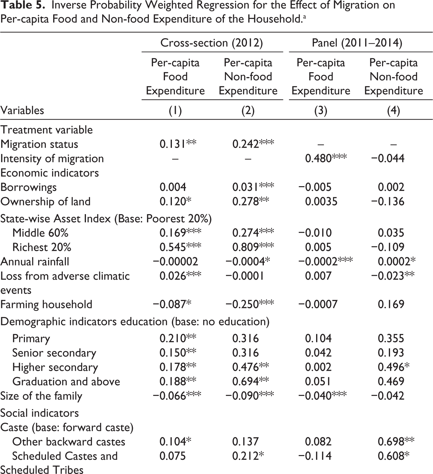
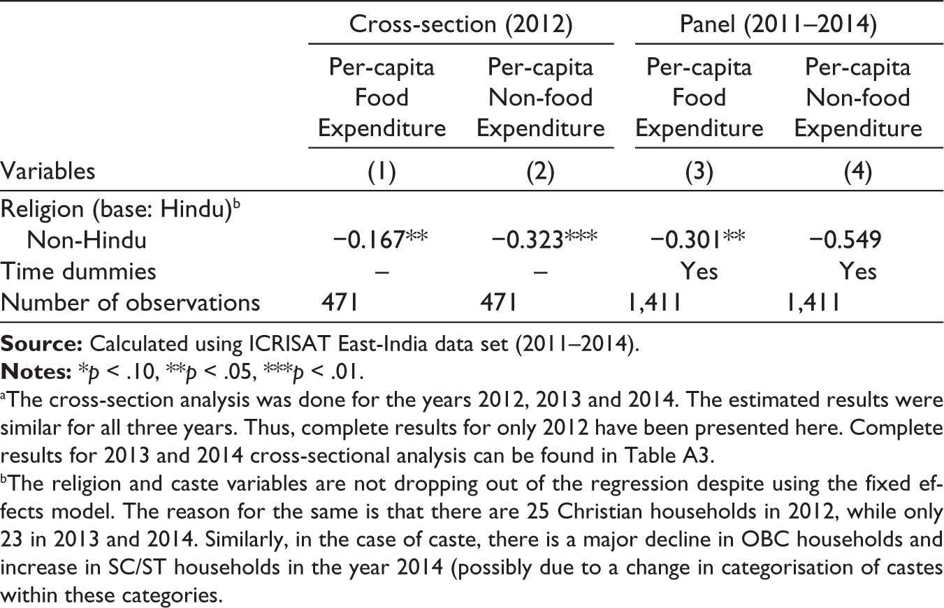
^aThe cross-section analysis was done for the years 2012, 2013 and 2014. The estimated results were similar for all three years. Thus, complete results for only 2012 have been presented here. Complete results for 2013 and 2014 cross-sectional analysis can be found in Table A3.

^bThe religion and caste variables are not dropping out of the regression despite using the fixed effects model. The reason for the same is that there are 25 Christian households in 2012, while only 23 in 2013 and 2014. Similarly, in the case of caste, there is a major decline in OBC households and increase in SC/ST households in the year 2014 (possibly due to a change in categorisation of castes within these categories.

Determinants of Intensity of Seasonal Migration

Economic motives are considered to be the most fundamental when deciding whether the household should engage in migration or not. In this study, if a household experiences any increase in the loss occurring on account of sudden climatic change, the intensity of migration increases. Thus, as households experience monetary loss due to climate changes, they start engaging in migration more frequently in order to cope with the risk of falling incomes. Similar results were found in the earlier studies for southern India (Pradhan & Narayanan, 2019, 2020). Moreover, even after controlling for the benefits received from government schemes, its insignificance in the results indicates towards the inadequacy in providing the required cushioning to the households against economic distress. Thus, migration becomes a coping strategy and mitigates the risk of uncertain incomes.

Further, operational landholdings have a significant and negative effect where an increase of one unit in operational landholdings is likely to reduce the intensity of migration by 1.3 percentage points. Greater operational landholdings increase the household’s farm income, and thus provide overall economic stability. As a result, the intensity of migration is lower for such households (Akhter & Bauer, 2014; Keshri & Bhagat, 2012; Pradhan & Narayanan, 2019).

The results further indicate a significant and positive coefficient for the size of the family, implying that a larger family engages in the seasonal migration with a greater intensity. This result is aligned with the standard literature on migration, where a higher family size implies a higher financial burden for the entire household (Pradhan & Narayanan, 2019; Zhu, 2002). In order to deal with the increased financial burden, not only are the households more likely to engage in migration, but they also migrate more frequently (depicted by higher person-months engaged in migration at the household level).

Wage differential is one of the primary motives in migration, proven theoretically and empirically in numerous studies (Harris & Todaro, 1970; Munshi & Rosenzweig, 2016; Nakosteen & Zimmer, 1982; Todaro, 1969; Zhu, 2002). In this study, however, wage differential turned out to be insignificant, indicating towards seasonal migration where migration is undertaken as a risk-diversifying strategy. Under such a scenario, it is not the rural–urban wage difference that motivates the household to migrate but it is undertaken as a coping strategy to diversify the risk arising from rural farm employment (Stark & Levhari, 1982). Similarly, if the household is receiving any benefit from the government schemes, it has a negative but insignificant effect on the intensity of migration of the household. This highlights that the government schemes related to employment remained ineffective in providing more secured livelihood to reduce distress-related seasonal migration from the rural villages.

Consumption of Left-behind Families

The results for the IPW regressions in the case of cross-sectional data for the year 2012 (columns 1 and 2 of Table 5) show that ATT of the decision to migrate is significant and increases the per-capita food and non-food expenditure by 13.1% and 24.2%, respectively. This finding suggests that the decision to send a family member away for employment improves the overall livelihood of the left-behind families in the villages as compared to the households that did not engage in migration. Also, the magnitude of the increase in non-food expenditure is higher than the food expenditure for migrant households, as with the increase in income, the share of food expenditure in the total expenditure of the household starts declining. At the same time, other expenses take up a larger share (Zarate-Hoyos, 2004). Beyond a level of consumption, the family starts spending on other necessities (such as household utilities and short-term consumer durables) required for their day-to-day survival.

Further, the results for other control variables show that the expenditure for both food and non-food categories is significantly higher for the migrant households if they are already better off. The migrant households that own any land in the villages, as well as those with the higher ownership of consumer durables (richest 20% category), experience higher food and non-food expenditure. Further, we find that the role of climatic conditions is crucial in this case as well, as an increase in rainfall leads to a lower non-food expenditure. On the other hand, experiencing loss due to adverse climate change shifts the focus to essential expenditures, thus, the households incur higher food expenditures in order to maintain their basic subsistence levels. Also, non-food expenditure is higher if the household has borrowings, while if the household’s dominant occupation is farming, they experience lower food as well as non-food expenditure indicating towards economic distress in farming activities.

Moving on to the household characteristics, the size of the family has a negative relation with both food as well as non-food expenditure. In the case of per-capita food expenditure, it can be argued that a larger size of the family entails a reduction in the per-capita food expenditure due to the presence of economies of scale as the marginal cost for cooking for an additional individual keeps on falling (Zarate-Hoyos, 2004). The findings in this study depict a trend of marginalised households experiencing improved consumption after migration as households belonging to the OBC category experience higher food expenditure and households belonging to Scheduled Castes and Scheduled Tribes (SC and ST) category experience higher non-food expenditure compared to forward caste households. In contrast, in the case of religion, the non-Hindu households experience lower food as well as non-food expenditure.

Additionally, we present the results taking the intensity of seasonal migration as the treatment variable for the panel data of 2011–2014 in columns 3 and 4 of Table 5. The results show a positive and significant effect of the intensity of migration on the per-capita food expenditure. However, in the case of the non-food expenditure, the effect was insignificant. This implies that as the intensity of migration is increasing, the migrant households spend an increasing proportion of the increased income on food-related expenditure highlighting the greater importance given to food expenditure in the overall consumption expenditure of the household. This is especially true in the case of poorer households experiencing economic distress and the primary concern is to fulfil the basic food requirements of the entire family (Castaldo & Reilly, 2007).

In the case of both per-capita food and non-food expenditure, rainfall in the previous period and the size of the family is significantly affecting the expenditure. The negative coefficient of rainfall in the case of food expenditure indicates better rainfall leading to more produce and lowering of agricultural prices as well as the fact that close to 60% of the households are farming households and consumption out of their own produce reduces their food expenditure (Hossain & Ahsan, 2022). As a result, the household’s spending on food is decreasing with the increase in rainfall. Moreover, this additional income due to increased rainfall is spent towards the non-food expenses of the household. Further, the coefficient for family size remains negative for the panel analysis as well as per-capita food expenditure of the household decreases with the increase in the intensity of migration. The households experiencing any loss due to adverse climatic conditions reduce their non-food consumption to cope with the economic distress. Moreover, taking forward caste as the base, the non-food expenditure of the marginalised households belonging to OBC and SC and ST categories increases as they receive the private transfers. In the case of religion, non-Hindu households experience a decrease in the per-capita food expenditure.

Robustness Check

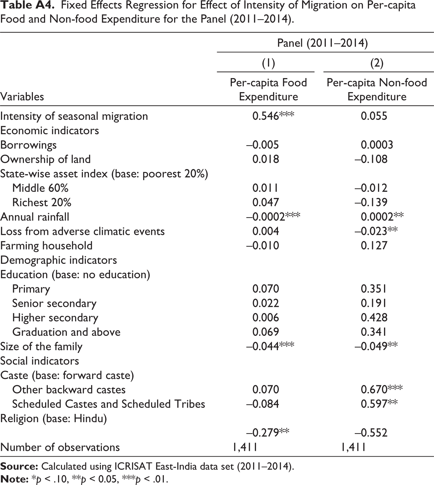
For the robustness check analysis, where we try to estimate effect of intensity of migration on consumption expenditure of the household by taking the average values of the explanatory variables, the results show a similar story as the effect of intensity of seasonal migration is significant for per-capita food expenditure while insignificant in the case of per-capita non-food expenditure. The results for other control variables are also stable with similar outcomes across both specifications. Thus, after using averages of the variables across the period of 2012–2014, we can conclude that the results are stable across the two specifications. This can imply that the average characteristics of the households remain consistent over the years and thus, using the propensity score for year 2012 or with averages across three years gives similar outcomes. The results of this robustness check are presented in Table A4.

To sum up, we find evidence of economic distress increasing the intensity of migration in rural villages of Bihar, Jharkhand and Orissa. External shocks in the form of adverse climatic events are increasing the intensity of migration of the household. Furthermore, as in the theory of NELM (Stark & Bloom, 1985), the collective decision by the household to engage in migration plays a significant role in improving the livelihood of the left-behind families through increased consumption expenditure.

Conclusion

In this study, we first examine the determinants of intensity of seasonal migration at the household level and then find out whether migration improves the food and non-food expenditure of left-behind families. The empirical results indicate distress migration, where migration is undertaken as a coping mechanism to deal with unfavourable economic conditions. The results highlight the dominance of push factors originating in rural areas in increasing the intensity of migration. While the role of government employment schemes remains insignificant in this study, the fluctuations in the climatic conditions significantly affect rural households that are mainly dependent on agriculture for their livelihood. Therefore, any negative shock through adverse climatic events leads to increased migration from the households. Further, lesser the operational landholdings of the household, greater the intensity of migration. In contrast to the expectations based on several empirical studies, the urban–rural wage differential is insignificant in our analysis, highlighting the nature of seasonal migration where the motive is to diversify the risk and maximising income of the household during slack season of agricultural when lesser employment opportunities are available in the rural areas. Thus, migration takes place due to the push factor of unavailability of employment opportunities rather than the pull of urban–rural wage differential.

Based on the results from IPW regression analysis for both cross-sectional data and panel data, we can conclude that the decision to migrate and the intensity of migration positively affect household consumption expenditures. While the effect on per-capita food expenditure was consistent under both methods, the effect of migration on the per-capita non-food expenditure is significant only in the case of cross-sectional analysis. The results emphasise the role of seasonal migration as an additional income source for left-behind families in rural Indian villages.

The findings of this study are confined to only three states in India and highlight the need for a wider data set to make more general policy-relevant suggestions. With a nationwide data set, it will also be possible to explore regional variations which will give meaningful insights in analysing the role that government schemes related to employment and credit can play in migration. Nonetheless, the results reiterate the seasonal migration as a coping mechanism for rural households to deal with income fluctuations and climate shocks.

Footnotes

Declaration of Conflicting Interests

The authors declared no potential conflicts of interest with respect to the research, authorship and/or publication of this article.

Funding

The authors received no financial support for the research, authorship and/or publication of this article.

Appendix

Table A4.

Fixed Effects Regression for Effect of Intensity of Migration on Per-capita Food and Non-food Expenditure for the Panel (2011–2014).

Variables	Panel (2011–2014)
	(1)	(2)
	Per-capita Food Expenditure	Per-capita Non-food Expenditure
Intensity of seasonal migration	0.546***	0.055
Economic indicators
Borrowings	–0.005	0.0003
Ownership of land	0.018	–0.108
State-wise asset index (base: poorest 20%)
Middle 60%	0.011	–0.012
Richest 20%	0.047	–0.139
Annual rainfall	–0.0002***	0.0002**
Loss from adverse climatic events	0.004	–0.023**
Farming household	–0.010	0.127
Demographic indicators
Education (base: no education)
Primary	0.070	0.351
Senior secondary	0.022	0.191
Higher secondary	0.006	0.428
Graduation and above	0.069	0.341
Size of the family	–0.044***	–0.049**
Social indicators
Caste (base: forward caste)
Other backward castes	0.070	0.670***
Scheduled Castes and Scheduled Tribes	–0.084	0.597**
Religion (base: Hindu)
	–0.279**	–0.552
Number of observations	1,411	1,411

Source: Calculated using ICRISAT East-India data set (2011–2014).

Note: *p < .10, **p < 0.05, ***p < .01.

Notes

References

Adams Jr.

R. H.

, & Cuecuecha

(2010). Remittances, household expenditure and investment in Guatemala. World Development, 38(11), 1626–1641.

Akhter

, & Bauer

(2014). Household level determinants of rural–urban migration in Bangladesh. International Journal of Humanities and Social Sciences, 8(1), 24–27.

Antman

F. M.

(2013). The impact of migration on family left behind. In International handbook on the economics of migration (pp. 293–308). Edward Elgar Publishing.

Bhagat

R. B.

(2010). Internal migration in India: Are the underprivileged migrating more? Asia Pacific Population Journal, 25(1), 27–45.

Caliendo

, & Kopeinig

(2008). Some practical guidance for the implementation of propensity score matching. Journal of Economic Surveys, 22(1), 31–72.

Castaldo

, & Reilly

(2007). Do migrant remittances affect the consumption patterns of Albanian households? South-Eastern Europe Journal of Economics, 5(1), 25–54.

Chandrasekhar

, Das

, & Sharma

(2015). Short-term migration and consumption expenditure of households in rural India. Oxford Development Studies, 43(1), 105–122.

Choksi

, Singh

, Mondal

, Nagendra

, Urpelainen

, & DeFries

(2021). Sensitivity of seasonal migration to climatic variability in central India. Environmental Research Letters, 16(6), 064074.

Clément

(2011). Remittances and household expenditure patterns in Tajikistan: A propensity score matching analysis. Asian Development Review, 28(2). 10.2139/ssrn.2001145

10.

Datta

(2020). Circular migration and precarity: Perspectives from rural Bihar. The Indian Journal of Labour Economics, 63(4), 1143–1163.

11.

Démurger

, & Wang

(2016). Remittances and expenditure patterns of the left behinds in rural China. China Economic Review, 37, 177–190.

12.

Deshingkar

(2017). Towards contextualised, disaggregated and intersectional understandings of migration in India. Asian Population Studies, 13(2), 119–123.

13.

Deshingkar

, & Start

(2003). Seasonal migration for livelihoods in India: Coping, accumulation and exclusion (Vol. 111). Overseas Development Institute.

14.

Dodd

, Humphries

, Patel

, Majowicz

, & Dewey

(2016). Determinants of temporary labour migration in southern India. Asian Population Studies, 12(3), 294–311.

15.

Economic Survey of India. (2022). Government of India. https://www.indiabudget.gov.in/economicsurvey/

16.

Filmer

, & Pritchett

L. H.

(2001). Estimating wealth effects without expenditure data—or tears: An application to educational enrolments in states of India. Demography, 38(1), 115–132.

17.

Haberfeld

, Menaria

R. K.

, Sahoo

B. B.

, & Vyas

R. N.

(1999). Seasonal migration of rural labor in India. Population Research and Policy Review, 18, 471–487.

18.

Harris

J. R.

, & Todaro

M. P.

(1970). Migration, unemployment and development: A two-sector analysis. The American Economic Review, 60(1), 126–142.

19.

Hossain

, & Ahsan

R. N.

(2022). When it rains, it pours: Estimating the spatial spillover effect of rainfall. Environmental and Resource Economics, 82(2), 327–354.

20.

ICRISAT East India Data Set. (2011–2014). https://vdsa.icrisat.ac.in/vdsa-database.aspx

21.

Jimenez-Soto

E. V.

, & Brown

R. P.

(2012). Assessing the poverty impacts of migrants’ remittances using propensity score matching: The case of Tonga. Economic Record, 88(282), 425–439.

22.

Keshri

, & Bhagat

R. B.

(2012). Temporary and seasonal migration: Regional pattern, characteristics and associated factors. Economic & Political Weekly, 47(4), 81–88.

23.

Koc

, & Onan

(2004). International migrants’ remittances and welfare status of the left-behind families in Turkey. International Migration Review, 38(1), 78–112.

24.

Kuhn

, Everett

, & Silvey

(2011). The effects of children’s migration on elderly kin’s health: A counterfactual approach. Demography, 48(1), 183–209.

25.

Lucas

R. E.

, & Stark

(1985). Motivations to remit: Evidence from Botswana. Journal of Political Economy, 93(5), 901–918.

26.

Marta

, Fauzi

, Juanda

, & Rustiadi

(2020). Understanding migration motives and its impact on household welfare: Evidence from rural–urban migration in Indonesia. Regional Studies, Regional Science, 7(1), 118–132.

27.

McKenzie

, Stillman

, & Gibson

(2010). How important is selection? Experimental vs. non-experimental measures of the income gains from migration. Journal of the European Economic Association, 8(4), 913–945.

28.

Mincer

(1978). Family migration decisions. Journal of Political Economy, 86(5), 749–773.

29.

Morten

(2019). Temporary migration and endogenous risk sharing in village India. Journal of Political Economy, 127(1), 1–46.

30.

Munshi

, & Rosenzweig

(2016). Networks and misallocation: Insurance, migration and the rural–urban wage gap. The American Economic Review, 106(1), 46–98.

31.

Nakosteen

R. A.

, & Zimmer

M. A.

(1982). The effects of earnings of interregional and interindustry migration. Journal of Regional Science, 22(3), 325–341.

32.

Nienkerke

I. M.

, Thorat

, & Patt

(2023). From distress migration to selective migration: Transformative effects of agricultural development on seasonal migration. World Development Perspectives, 29, 100483.

33.

Papke

L. E.

, & Wooldridge

J. M.

(2008). Panel data methods for fractional response variables with an application to test pass rates. Journal of Econometrics, 145(1–2), 121–133.

34.

Piracha

, & Saraogi

(2017). Remittances and migration intentions of the left-behind. Migration and Development, 6(1), 102–122.

35.

Pradhan

K. C.

, & Narayanan

(2019). Intensity of labour migration and its determinants: insights from Indian semi-arid villages. Asia Pacific Journal of Regional Sciences, 3, 955–994.

36.

Pradhan

K. C.

, & Narayanan

(2020). Does climate risk induce labour migration? Evidence from semi-arid tropics region of India. Journal of Public Affairs, 22(1), e2323.

37.

Randazzo

, & Piracha

(2019). Remittances and household expenditure behaviour: Evidence from Senegal. Economic Modelling, 79, 141–153.

38.

Rapoport

, & Docquier

(2006). The economics of migrants’ remittances. Handbook of the Economics of Giving, Altruism and Reciprocity, 2, 1135–1198.

39.

Ravenstein

E. G.

(1885). The laws of migration. Royal Statistical Society.

40.

Stark

, & Bloom

D. E.

(1985). The new economics of labour migration. The American Economic Review, 75(2), 173–178.

41.

Stark

, & Levhari

(1982). On migration and risk in LDCs. Economic Development and Cultural Change, 31(1), 191–196.

42.

Stark

, & Lucas

R. E.

(1988). Migration, remittances, and the family. Economic Development and Cultural Change, 36(3), 465–481.

43.

Todaro

M. P.

(1969). A model of labour migration and urban unemployment in less developed countries. The American Economic Review, 59(1), 138–148.

44.

Wang

, Liu

, & Yan

(2021). Temporary versus permanent migration: The impact on expenditure patterns of households left behind. Review of Economics of the Household, 19, 873–911.

45.

Yuni

D. N.

, Urama

N. E.

, & Urom

C. O.

(2018). Migrant remittances and household expenditure patterns: Case study of Enugu and Anambra states of Nigeria. World Applied Sciences Journal, 36(2), 319–327.

46.

Zarate-Hoyos

G. A.

(2004). Consumption and remittances in migrant households: Toward a productive use of remittances. Contemporary Economic Policy, 22(4), 555–565.

47.

Zhu

(2002). The impacts of income gaps on migration decisions in China. China Economic Review, 13, 213–230.

Intensity of Seasonal Migration and Its Impact on Household Consumption: Analysis of East Indian Villages

Abstract

Keywords

Introduction

Conceptual Background

Data and Variables

Economic Indicators

Demographic Indicators

Social Background

Econometric Methodology

Determinants of Intensity of Seasonal Migration

Migration and Household Consumption Expenditure

Empirical Results and Discussion

Determinants of Intensity of Seasonal Migration

Consumption of Left-behind Families

Robustness Check

Conclusion

Footnotes

Declaration of Conflicting Interests

Funding

Appendix

Notes

References