Sage Journals: Discover world-class research

Abstract

We estimate the returns (measured by hourly earnings) to education, experience, and social networking in India using individual-level panel data from the India Human Development Surveys. We combined the two latest waves of this survey using individual-level identifiers to generate a balanced panel and merged it with various household characteristics. We provide estimates of private returns for an additional year of education and experience by consumption quintiles, gender, caste, and religion in a fixed-effects Heckman model that controls for selection bias. This methodology improves upon estimates of all earlier studies on earnings in India, as most of the literature has relied on cross-section data or pseudo-panel data. We also examine the impact of social networking on earnings, which is under-explored in nationwide studies in India. We find that education significantly and positively affects earnings for all consumption quintiles, gender, caste (except schedule castes), and religious groups. Among economic groups, the highest returns are observed for the third quintile above the poverty line. Returns to females for an additional year of education are nearly double that of males but the difference in starting earnings keeps earnings of males higher for long periods. Among the castes, scheduled castes have the highest returns to education and other minorities among religious groups. Social networking positively impacts males, Hindus, and the quintile just above the poverty line. Experience positively impacts women’s earnings, general caste and scheduled caste, Hindus and Other minorities and two consumption quintiles (two and five) above the poverty line.

Plain Language Summary

Impact of Education, Experience, and Social Networks Impact Earnings in India by Class, Gender, Caste and Religion

Purpose: Enhancing human capital is critical for India’s development. It would help overcome existing labor market hierarchies based on economic class, gender, religion, and caste. We study the impact on private earnings of (a) an additional year of education and experience, and (b) social networking. Methods: We use an individual level panel dataset assembled from the two latest rounds of the Indian Human Development Survey (I&II). Our Heckman type earnings equation controls for selection bias. Results: An additional year of education increased earnings between (a) 2.4% and 8.8% among different consumption quintiles (b) 3.7% for males to 5.2% for females, (c) 1.5% (STs), to 5.9% (SCs), and (d) 2.3% (Muslims), to 9.9% (Other Minorities). Experience increased earnings of two economic groups, females, the General and Scheduled castes, and of Hindus and Other Minorities. Social networking increased earnings of males, Hindus, and one economic quintile. Conclusions: Higher marginal returns to education for females justifies greater investment in women’s education. Lower returns on education among STs and Muslims indicate the need for affirmative action for these groups. The positive returns to education for the poor suggests that anti-poverty programs in combination with educational opportunities for the less privileged would meet the goals of social justice. Implications Better education (SDG4) would help achieve gender equality (SDG5), and social justice for marginalized (economic, caste and religious) groups (SDG1, SDG10). Limitations: We were unable to account for ability bias. Stratification by state and sector would provide better estimates.

Keywords

economics education economic science social sciences labor and demographic economics educational research education social structure sociology disparities labor and labor movements sociology of work

Introduction

Do women and men get similar private returns to education and experience in India? Do caste, religion and social networking play a role in determining wages? If so, to what degree? These questions continue to hold center stage in household decision-making and development policy-making in countries such as India. They echo similar concerns in other parts of the world, including developed countries where identity issues—predominantly based on economic status, caste, race, gender, and religion—have been sites for discrimination.

In this paper, we re-examine the issue of private returns to education (earnings) in India. We use data from two rounds of the India Human Development Survey (IHDS) to construct a balanced individual-level panel data set, subsequently merged with household characteristics. The IHDS data set has been used in individual and household panel models (Akter & Chindarkar, 2020; Azam, 2018; E. Chatterjee & Sennott, 2021; Tamuly & Mukhopadhyay, 2022). However, to the best of our understanding, this is the first attempt to explain earnings in India with an individual panel data model, with individual-level fixed effects from a nationwide survey. We follow the Heckman selection model and use a new and improved command (xtheckmanfe) in Stata16.1 (Rios-Avila, 2021) to control for selection bias (Mundlak, 1978; Semykina & Wooldridge, 2010; Wooldridge, 2018).

We contribute to the literature by providing first estimates on the private returns to an additional year of education and experience by consumption quintiles, caste, gender, and religion. This improves upon Mitra’s (2019) method, which uses quintiles based on wages without separating the poor from the non-poor. Our analysis provides greater disaggregation, which can help in devising more effective and targeted policies for affirmative action. Previously, studies in India have employed a cross-section data set (Agrawal, 2014; Bairagya, 2020; Geetha Rani, 2014; Kingdon & Theopold, 2008; Mitra, 2019) or a quasi-panel (Bhattacharya & Sato, 2017; Mendiratta & Gupt, 2013) to study earnings in India. We believe our panel data approach improves upon estimates of all earlier studies on this subject. We also control for impacts of social networking which is less explored in wage determination models.

We found that education has a significant and positive effect on earnings for all consumption quintiles, genders, castes, and religious groups. Among economic groups, the highest returns are observed for the third quintile above the poverty line. Returns of additional years of education (marginal increase) to females are nearly double that of males. Among the castes, scheduled castes have the highest returns to education and among religious groups other minorities have the highest returns. Experience was found to be significant for two consumption quintiles above the poverty line, females, general castes and scheduled castes, Hindus and other religious Minorities. We also learned that social networking has an impact on the earnings of males, Hindus, and the quintile just above the poverty line. Our study also adds to the nascent literature on the impact of social networking on earnings in India.

Literature Review

Education is considered an investment in human capital which provides a pathway to overcome socio-economic and identity-based barriers. Accordingly, the human capital framework is often used to explain the earnings of individuals as a return on investment following the seminal contributions of Mincer (1958), Schultz (1961), and Becker (1962). An extensive empirical literature has emerged based on this framework (Acemoglu & Autor, 2012; N. Angrist et al., 2021; Beam et al., 2020; Becker, 1994; Collin & Weil, 2020; England & Folbre, 2023; Faggian et al., 2019; Goldin, 2016; H. A. Patrinos & Psacharopoulos, 2020). Conventional wage determination models use ordinary least squares (OLS) methods, but these have been demonstrated to suffer from selectivity and endogeneity bias (J. J. Heckman et al., 2006; Wooldridge, 2018). J. Heckman (1974) provides a mechanism to overcome the problem of selection bias in Mincer’s original formulation (Mincer, 1974). Apart from cross-country studies (H. A. Patrinos & Psacharopoulos, 2020; Peet et al., 2015), the Heckman selection model has since been used to estimate returns on education in different parts of the world such as the United States (J. D. Angrist & Krueger, 1991; J. Heckman & Polachek, 1974), Europe (Harmon et al., 2001), and China (Li, 2003).

The modified version of Mincer’s earnings function has been used to study the Indian labor markets (Bhaumik & Chakrabarty, 2008; Jacob, 2018; Vasudeva Dutta, 2006). The most widely used data set is from the National Sample Survey Organisation (NSSO), now renamed as the National Statistical Office (NSO) (Mohanty, 2021). The limitation of the NSSO data sets is that they are not amenable to panel data analysis directly, as they do not track the same household over time. Since cross-sectional studies have limitations and their findings are considered less reliable, panel data sets are preferred. Three such nationwide data sets are currently available in India: the India Human Development Surveys (IHDS) (Azam et al., 2013), the Periodic Labor Force Survey (PLFS) (NSO, 2021), and the Consumer Pyramids Household Survey (CPHS) of the Centre for Monitoring Indian Economy (CMIE) (Mamgain, 2021). The IHDS data has been used by numerous studies in the past (Akter & Chindarkar, 2020; Azam et al., 2013; E. Chatterjee & Sennott, 2021; Sarkar et al., 2019; Tamuly & Mukhopadhyay, 2022).

The PLFS has been in the public domain since 2017 to 2018 (NSO, 2021). It collects household data every quarter, however, an individual household is likely to be asked to provide information—in the form of a rotational panel—only once a year. This type of panel data has been used by Sengupta (2023) and Singha Roy (2020) among others. On the other hand, the CPHS data set has been tracking the consumption of randomly selected households thrice a year since 2016. However, unlike the IHDS and the PLFS, this data set is subscription-based.

A few studies have created a regional pseudo-panel data set using district identifiers as proposed by Deaton (1985) and, thus, overcome the problems posed by estimates of cross-section data. Bhattacharya and Sato (2017) use this technique to analyze the effect of socioeconomic factors on the real wage rate of male workers in India. They find that caste and religion were not significant determinants of wages. This is contrary to the understanding of the Indian labor market, where gender, caste, and religion have been found to influence wages (Agrawal, 2014; Sengupta & Das, 2014).

Education is an important form of investment in the human capital (Becker, 1994). The gains from higher educational attainment can translate into higher earnings as well as create pathways for social mobility through historically determined social hierarchies, which are based on gender, caste, and religion (Sen, 2000, 2001). In this study, “earnings” is used interchangeably with wages and salaries received by individuals. In the Indian context, studies have shown evidence of labor market discrimination based on gender (Chakraborty et al., 2020), caste (Kumar & Hashmi, 2020; Madheswaran & Singhari, 2016), and religion (Dhesi & Singh, 1989). Therefore, to estimate the degree of discrimination, it is important to measure the differences in individual earnings on the basis of known social characteristics.

Material and Methods

Data

We use two of the latest IHDS rounds (round 1 conducted in 2004–2005, hereafter IHDS I, and round 2 conducted in 2011–2012, hereafter IHDS II). This data set emerged as a collaborative research program between the National Council of Applied Economic Research, New Delhi, India, and the University of Maryland, United States (Desai & Vanneman, 2005, 2015). Certain features of the IHDS data set make it unique in comparison to the commonly used data sets in Indian literature. First, topics in IHDS extend across indicators of caste, community, consumption, the standard of living, energy use, income, agriculture, employment, government subsidies, education, social and cultural capital, household and family structure, marriage, gender relations, fertility, health, village, infrastructure, among others. Second, the human development indicators documented are extensive and the data set contains a wide array of contextual measures. Third, the panel components allow for richer inferences to be drawn between time periods.

IHDS I is a nationally representative data set, covering 41,554 households in 1,503 villages and 971 urban blocks across India. The sample consists of 26,734 rural and 14,820 urban households. Of the 593 districts in India in 2001, 384 were included in IHDS I. The household sample in IHDS I is a composite of several separate subsamples that were each drawn somewhat differently. It contains a subsample of re-interviewed households, last interviewed in 1994 to 1995 for the Human Development Profile of India (HDPI). Therefore, the data set includes 13,900 households from the HDPI and a subsample of 27,654 new households. IHDS II covers 42,152 households in 384 districts, 1,420 villages, and 1,042 urban blocks located in 276 towns and cities. Most of the households from IHDS-I (83%) were re-interviewed for IHDS II. Both surveys cover all states and union territories of India except Andaman/Nicobar and Lakshadweep.

We first downloaded the Stata-formatted files from the IHDS repository, which is free to download for researchers after registration (Desai & Vanneman, 2005, 2015). We merged the individual records from the two rounds of IHDS and arrived at 150,995 individuals. Only individuals who had been interviewed in both rounds were retained for observation. The method to identify and merge these files is available from the IHDS repository. On completion of the merger, we cross-checked the resultant number of observations with IHDS documents to ensure that we had the same numbers as were derived from the master notes. The merged data set provided a balanced individual-level panel. Thereafter, we merged the household-level dataset from the two rounds to obtain a balanced household-level panel. Next, we linked the individual characteristics with the household characteristics by merging the individual panel with the household panel, which provided us with an extensive panel data set for a comprehensive analysis.

The dependent variable in our analysis is the natural log value of the hourly earnings of individuals (lnHourly_Earnings). As discussed earlier, in this context, earnings include wages as well as salary work. IHDS I and II collected information pertaining to wage and salary work under the income and social capital heads. We have used the variables WS8hourly (hourly wage total) and WSEARNHOURLY (hourly wage and bonuses) from the IHDS I and II databases, respectively. To make monetary values in the two rounds—such as earnings and consumption—comparable, we have used a deflation factor provided by IHDS, which normalizes the 2005 values and makes them comparable to the 2012 values.

Sub-Sample Selection

Since our focus is on the earnings of eligible persons in the labor force, we have restricted our analysis to individuals belonging to the working age group (15–64 years)—the age group considered eligible to participate in the labor force (The World Bank, n.d.). To study the variation in earnings and education between the two rounds, we have excluded (a) those who were not interviewed in both rounds, (b) those who were still enrolled in school or college during IHDS II and thus ineligible to be in the labor market, and (c) those whose education level did not change between the two rounds.

Variables

Our dependent variable is the natural log of hourly earnings (lnHourly_Earnings) reported by each individual in the outcome equation, in keeping with the literature on this subject (Eisnecker & Adriaans, 2023; J. Heckman & Polachek, 1974; Hoffmann & Kassouf, 2005). The dependent variable in the selection equation is a binary variable that indicates whether a person is in the labor force or not (Labor Force Participation). We constructed this variable based on whether a person reported an earning. Among the covariates, we have used variables that are commonly used in the literature for predicting earnings: the individual’s education in completed years (Education), potential experience (Experience), and the square of potential experience (Experience_square).

We have used family characteristics like the number of children (Nchildren) (Mroz, 1987), marital status (Married) (Comola & de Mello, 2013), and the number of adults in a household (Nadults) (Ashraf et al., 2013; Kugler & Kumar, 2017), among others. In India, women are anticipated to exit the labor market when they become mothers (Jaumotte, 2003). This can be partly attributed to the patriarchal structure of Indian society, as the main burden of child-rearing falls on the mother (Bhambhani & Inbanathan, 2018). Therefore, variable Nchildern adversely influences women’s presence in the labor market and the nature of the employment (Chun & Oh, 2002).

The family’s economic status is often reflected in their consumption expenditures. We have used household consumption expenditure to first classify households as below or above poverty. To create consumption quintiles, the entire sample was divided into two broad groups by level of consumption: those below the poverty line (BPL) and those above it (APL). We further disaggregated the APL group into five quintiles (labeled APL1 (low) to APL5 (high)).

Gender identities have been widely acknowledged as a determinant of employment and earnings across the world (Blau et al., 2012) and studies show that a gender wage gap exists in the labor market (Sengupta & Das, 2014). We have included the variable Female (binary values with Female = 1, Male = 0) to examine any gap in returns to education.

Social groups in India are broadly classified along two identities—caste and religion. The role of caste and religion in determining earnings has been examined before (Arabsheibani et al., 2018; Bhaumik & Chakrabarty, 2010; Geetha Rani, 2013). India also has a unique social hierarchical system based on caste (Deshpande, 2011), which has well-known implications for economic outcomes (Bhaumik & Chakrabarty, 2008; Lolayekar & Mukhopadhyay, 2020). The hierarchy places the general castes at the top of the social ladder, followed by the other backward castes (OBC) and scheduled castes (SC). The scheduled tribes (ST) are strictly not part of the caste system. Rather, they are indigenous groups and are ranked often at the bottom of the social hierarchy (GoI, 2016; Mosse, 2018). There have been many social movements to abolish social hierarchies based on caste (Ray & Katzenstein, 2005). The state policy has also undertaken affirmative action by providing educational and employment reservations for lower castes (Deshpande, 2013). However, there is evidence that caste hierarchies still exist (Arabsheibani et al., 2018). In IHDS I, there were five caste categories—namely Brahmin, OBC, SC, ST and others. In IHDS II, there were six caste categories—namely Brahmin, Forward /General (except Brahmin), OBC, SC, ST and others. In order to make the categorization uniform across the two rounds and to match the government classification for employment reservations, we have classified the caste data into four categories, namely General (Forward, Brahmin and Others together), OBC, SC and ST. We created categorical groups as a variable Caste (General = 1, OBC = 2, SC = 3, ST = 4).

Religion has been identified as a determinant of economic outcomes (Barro & McCleary, 2003). It is recognized as a site for determining social and economic hierarchy. Studies have found significant differences in development indicators based on religious groupings (Geetha Rani, 2013). A government report found that Muslims as a group have the lowest development indicators among all religious minority groups in India (GoI, 2006). In IHDS I and IHDS II, there were nine religion categories—namely Hindu, Muslim, Christian, Sikh, Buddhist, Jain, Tribal, Others, and None. In order to make the categorization tractable, we created three groups, namely Hindu, Muslims and Other minorities (which included all the remaining groups, i.e., Christian, Sikh, Buddhist, Jain, Tribal, Others and None). The new variable Religion was a categorical variable (Hindu = 1, Other minorities = 2, Muslims = 3).

Social networking has been found to influence individual earnings in China (Liu, 2017), United States (Smith, 2000), Sweden (Behtoui & Neergaard, 2010) as well as India (Deshpande & Khanna, 2021). We added an indicator of social networking to the outcome equation (Networking Intensity). We constructed this variable by utilizing information regarding a household’s membership in one or more social or economic networking groups (membership in co-operatives, caste or religious groups, self-help groups, among others) (Dasgupta, 2005; Deshpande & Khanna, 2021).

In keeping with the literature, we constructed a variable to measure potential experience, since the IHDS did survey the experience of individuals directly (Lemieux, 2006). This variable is equal to the respondent’s age minus the years of education minus 5 years (to account for preschool years as relevant in the Indian context). We have capped the maximum experience at 45 years (the gap between the entry and exit age group for labor force participation). It is debatable whether such an assumption is valid. We acknowledge that this assumption may not be universally valid but, under specific circumstances, it could reflect the labor market situation. We contend that during the years the two rounds of the IHDS surveys were conducted, the Indian economy experienced high growth and the labor market underwent informalisation. The data from the NSSO’s quinquennial rounds (2004–2005 and 2011–2012) suggests that the prevailing rates of unemployment in the overall population were 2.2% and 2.3% (Mehrotra, 2019). Therefore, even if there was underemployment in the economy, the actual percentage of unemployment recorded was relatively low.

Empirical Model

Mincer’s earliest form of the earnings function ran a single regression equation in the semi-log form (Mincer, 1974). The model used Education, Experience, and Experience_square as co-variates. Over the years, researchers have fed many variations in Mincer’s original model for use in different contexts. One of the reasons for using a quadratic form for experience was to account for any non-linear effect that it may have on earnings, which could emerge from a loss in productivity due to age. Mincer’s earnings function can be framed as:

\begin{matrix} lnHourly_Earnings \\ = f (Education, Experience, Experience_square) \end{matrix}

(1)

The early econometric method for estimating the Mincer earnings function used the ordinary least squares (OLS) equation (Hartog & Gerritsen, 2016; Polachek, 2008). The econometric formulation of Equation 1 would then be stated as:

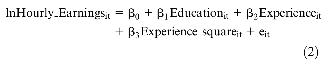
\begin{matrix} lnHourly_Earning s_{it} & = β_{0} + β_{1} Educatio n_{it} + β_{2} Experienc e_{it} \\ + β_{3} Experience_squar e_{it} + e_{it} \end{matrix}

(2)

where e_it = stochastic error term and β₁ =the average private returns to an additional year of education.

The coefficient of Experience_square (β₃) helps establish whether the relationship has any second-order effects. However, it has been recognized that OLS estimates suffer from at least two sources of bias—selectivity and ability bias (J. D. Angrist & Krueger, 1991). Selecting only those individuals who reported earnings to estimate the returns to an additional year of education could overestimate the effect of education. This error in estimation, using only the sub-sample of individuals who reported earnings, is called selection bias (J. Heckman, 1974; J. J. Heckman, 1976, 1979). The issue of endogeneity is the other bias common in these estimations (Card, 1999). Individuals may embody innate abilities or genetic traits that aid productivity over and above additional years of education. The average private return to additional years of education may be an overestimation due to these unobservable traits. Children with greater ability are more likely to continue in school than others. The returns to education may be overestimated in such cases as well (H. Patrinos, 2016).

These issues of specification and endogeneity bias have been the focus of more recent research in the area of human capital investment and, specifically, on returns to education. Different methods have been proposed to tackle the problem of endogeneity. The most popular one is the instrumental variable (IV) approach (Carneiro et al., 2011). Instruments are variables that are strongly correlated to the endogenous covariate but not correlated to the outcome variable (Briggs, 2004). The challenge in empirical studies has been to find effective instruments (J. D. Angrist & Krueger, 2001; Baltagi & Khanti-Akom, 1990). The current recommendation is to use an instrument or treatment that has been assigned randomly rather than an individual-related characteristic (Wooldridge, 2018).

In non-experimental data, the challenge of finding the right instrument has led researchers to abandon the IV method (Rossi, 2014; Truong et al., 2021), as weak instruments lead to greater bias than other techniques (Bound et al., 1995; Cruz & Moreira, 2005). For this reason, we have chosen to not use the IV method. Instead, we use the workhorse of such studies—the fixed-effects model with Heckman correction—to control for selection bias (Wooldridge, 2018), with longitudinal data to estimate fixed-effects models (Kamhöfer & Schmitz, 2016; Leigh, 2008). This model controls for average differences across individuals in any observable or unobservable predictors. The within-group estimate explains the effect of covariates on the earnings of an individual over time.

In the first stage (selection equation), we predicted participation in the workforce with instruments such as Married, Nchildren, and Nadults apart from the explanatory variables of the outcome equation (Semykina & Wooldridge, 2010). The selection equation is stated as:

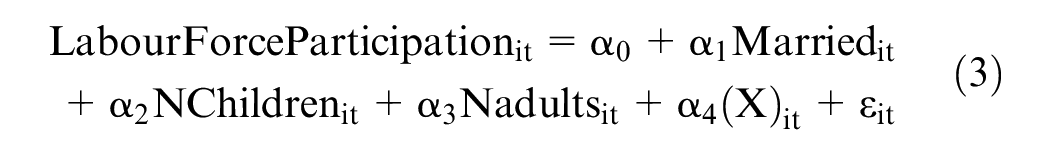
\begin{matrix} Labour Force Participatio n_{it} = α_{0} + α_{1} Marrie d_{it} \\ + α_{2} NChildre n_{it} + α_{3} Nadult s_{it} + α_{4} {(X)}_{it} + ε_{it} \end{matrix}

(3)

where X = the set of exogenous explanatory variables of the outcome equation indicated in Equation 4 and ε = stochastic error term.

In the second stage of the Heckman procedure (outcome equation), we used a semi-log polynomial model to allow second-order covariates for experience (Equation 4). The outcome equation is stated as:

\begin{matrix} lnHourly_Earning s_{it} = β_{0} + β_{1} Educatio n_{it} + β_{2} Experienc e_{it} \\ + β_{3} Experience_squar e_{it} + β_{4} Networking Intensit y_{it} \\ + β_{5} IM R_{it} + β_{6} Z_{it} + e_{it} \end{matrix}

(4)

where IMR = the inverse Mills ratio generated from the first stage selection equation, Z = the set of included instrumental variables from the selection Equation 3 (Married, NChildren, and Nadults), e = error term, i = ith individual, and t = year (2005 or 2012).

Econometric Models, Estimation, and Tests

First, we estimated the Mincer earnings function using fixed effect (FE) and random effect (RE) models (using the xtreg command in Stata 16.1). Then, we used the Hausman test (hausman command) to confirm that the FE model was more suitable for our analysis. Unlike earlier panel commands for the Heckman model, xtheckmanfe allows us to incorporate FE while addressing selection bias. This, we believe, is a methodological improvement over other previous studies (Briggs, 2004; Schwiebert, 2012), and our estimates update their results.

In the selection Equation 3, we used Married, Nadults, and Nchildren as excluded instruments (Comola & de Mello, 2013). These coefficients have been used in the recent literature as well (Beam et al., 2020; Sarkar et al., 2019). We anticipate that these variables could be acceptable instruments for selection in the labor market and tested the same for confirmation. The model also estimates a value for the inverse Mills ratio (IMR) by year, to test whether selectivity bias exists in the estimation. IMR is included in the outcome Equation 4 as a covariate. A significant value of IMR would imply the existence of selectivity bias. We estimate the coefficients for Equations 3 and 4 by consumption quintiles, caste, gender, and religion.

Results

We found that the (natural log of) average hourly earnings of an individual (overall) was 3.02 with a standard deviation of 0.8 (see Table 1). Average education was 7.9 years, with a standard deviation of 4.4 years (overall). The average experience was 19.5 years, with a standard deviation of 13.5 years (overall). Of the total sample, 62% were married and 39% were female. The average number of children was 1.54 and the adults were 3.47. The detailed groupwise values can be found in Supplemental Table S1.

Table 1.

Descriptive Statistics.

Variable	Description		Mean	Standard deviation	Minimum	Maximum	Observations
lnHourly_Earnings	Natural logarithm of hourly earnings observed	Overall	3.02	0.82	−0.84	6.92	21,413
		Between		0.77	−0.84	6.71	15,601
		Within		0.28	1.10	4.94	1.37
Education	Completed years of education	Overall	7.90	4.44	0	16	52,134
		Between		4.03	0	16	29,878
		Within		1.63	−0.10	15.90	1.74
Experience	Potential experience: {(age − education − 5) years}	Overall	19.51	13.53	0	45	52,378
		Between		13.62	0	45	29,889
		Within		2.71	−1.99	41.01	1.75
Experience square	Square of potential experience	Overall	563.77	629.60	0	2,025	52,378
		Between		627.80	0	2,025	29,889
		Within		138.98	−446.7	1,574.27	1.75
Networking intensity	Number of social or economic committees that household members were associated with	Overall	0.71	1.08	0	7	52,225
		Between		0.90	0	7	29,870
		Within		0.62	−2.79	4.21	1.75
Labor force participation	Binary variable (“1” if hourly earnings are observed, “0” otherwise)	Overall	0.41	0.49	0	1	52,378
		Between		0.43	0	1	29,889
		Within		0.25	−0.09	0.91	1.75
Married	Binary variable (“1” if individual is married, “0” otherwise)	Overall	0.62	0.49	0	1	52,378
		Between		0.46	0	1	29,889
		Within		0.18	0.12	1.12	1.75
Children	Number of children in the household	Overall	1.54	1.62	0	18	52,378
		Between		1.41	0	15	29,889
		Within		0.84	−4.96	8.04	1.75
Adults	Number of adults in household	Overall	3.47	1.74	0	18	52,378
		Between		1.50	0	18	29,889
		Within		0.90	−4.53	11.47	1.75
Consumption quintiles	“0” if below poverty line, “1” if lowest quintile above poverty line, and “5” if highest quintile above poverty line	Overall	2.66	1.75	0	5	52,365
		Between		1.54	0	5	29,889
		Within		0.89	0.16	5.16	1.75
Female	Binary variable (“1” if individual is female, “0” otherwise)	Overall	0.39	0.49	0	1	52,378
		Between		0.49	0	1	29,889
		Within		0.03	−0.11	0.89	1.75
Caste	Categories: “1” if general/others, “2” if other backward classes, “3” if scheduled castes, and “4” if scheduled tribes	Overall	2.11	1.10	1	4	52,310
		Between		0.81	1	4	29,888
		Within		0.78	0.61	3.61	1.75
Religion	Categories: “1” if Hindu, “2” if Other minorities, and “3” if Muslims	Overall	1.33	0.69	1	3	52,378
		Between		0.70	1	3	29,889
		Within		0.10	0.33	2.33	1.75

Source. Author’s calculations based on IHDS I and II (Desai & Vanneman, 2005, 2015).

We tested to ensure there was no multi-collinearity between the independent variables predicting earnings by using the variance inflation factor (VIF) measure. Our overall regression results showed VIF values between 1.44 and 1.88, which is considered moderate and requires no corrective action (Wooldridge, 2018).

To decide which of the FE and RE models was more suitable to this study (estimates can be found in Supplemental Table S2), we used the Hausman test (results can be found in Supplemental Table S3). The test statistic chi-square value was 186.29 (with a p-value .0000), which indicates rejection of the null hypothesis (of RE). Therefore, we accepted the alternate hypothesis that the FE model was better suited to our data.

The FE Heckman model (without disaggregation) suggests that earnings are positively and significantly affected by Education (see Table 2). The coefficient of Experience is positive and significant but that of the square term is negative and insignificant. Networking intensity has a positive and significant impact on earnings. The coefficients for IMR (2005 and 2012) are significant and indicate a selection bias, thus justifying the use of the selection model. Selection equation results are reported in Supplemental Table S4.

Table 2.

Panel Estimates From the Fixed-effects Heckman Model (full Sample) (Dependent Variable: lnHourly_Earnings).

Main equation	Estimate	SE	95% CI		P
Main equation	Estimate	SE	LL	UL	P
Education	0.0348***	0.004	0.026	0.0436	.0000
Experience	0.012**	0.005	0.0013	0.0226	.0290
Experience_square	−0.0001	0.000	−0.0003	0.0001	.3100
Networking Intensity	0.0164**	0.007	0.0031	0.0298	.0160
2012	0.2981***	0.057	0.1871	0.4092	.0000
IMR
2005	−0.2213***	0.038	−0.2956	−0.1471	.0000
2012	−0.3799***	0.049	−0.4765	−0.2832	.0000
Constant	1.5735***	0.056	1.4628	1.6843	.0000

Source. Author’s calculations based on IHDS I and II (Desai & Vanneman, 2005, 2015).

Note. Total N = 51,989. CI = confidence interval; LL = lower limit; UL = upper limit.

p < .1. **p < .05. ***p < .01.

By Consumption Quintiles

The results of the disaggregated estimation with six economic groups individually are presented in Table 3. We found that Education has a positive and significant impact on earnings across all quintiles. Experience too was positive and significant for APL 2 and APL 5. The squared effect was significant and negative for APL 5. Networking intensity was significant and positive for APL 1. The coefficients for IMR were significant for all quintiles (except BPL and APL 5) in 2005 and 2012, confirming the presence of selectivity bias. This also justifies the two-step approach of Heckman in our context. Selection equation results are reported in Supplemental Table S5.

Table 3.

Estimates From the Fixed-effects Heckman Selection Model by Consumption Quintiles (Dependent Variable: lnHourly_Earnings).

Main equation	BPL	APL1	APL2	APL3	APL4	APL5
Education	0.0241*** (0.0089)	0.0660*** (0.0144)	0.0489*** (0.0129)	0.0878*** (0.0213)	0.0786*** (0.0240)	0.0743*** (0.0200)
Experience	0.00108 (0.0163)	0.00763 (0.0282)	0.0443** (0.0190)	0.00894 (0.0296)	0.0206 (0.0276)	0.132*** (0.0188)
Experience_square	0.000292 (0.0003)	0.0000994 (0.0006)	−0.000198 (0.0005)	0.000260 (0.0006)	0.000595 (0.0005)	−0.00178*** (0.0004)
Networking Intensity	0.0336 (0.0217)	0.113*** (0.0388)	0.0359 (0.0522)	−0.0492 (0.0423)	−0.0282 (0.0389)	0.0230 (0.0277)
2012	0.246*** (0.0609)	−0.0550 (0.0830)	−0.182 (0.1242)	−0.0564 (0.1598)	−0.149 (0.1749)	−0.237* (0.1298)
IMR
2005	0.0319 (0.1047)	−0.321*** (0.1085)	−0.469*** (0.1070)	−0.414*** (0.0808)	−0.783*** (0.1033)	0.0866 (0.1103)
2012	−0.0308 (0.1446)	−0.217 (0.1730)	−0.473*** (0.1770)	−0.625*** (0.2053)	−1.013*** (0.2271)	0.199 (0.1589)
Constant	1.810*** (0.1319)	2.219*** (0.1389)	2.640*** (0.1243)	2.482*** (0.1157)	3.064*** (0.1779)	1.451*** (0.1935)

Source. Author’s calculations based on IHDS I and II (Desai & Vanneman, 2005, 2015).

Note. Standard errors in parentheses.

*p < .1. **p < .05. ***p < .01.

By Gender

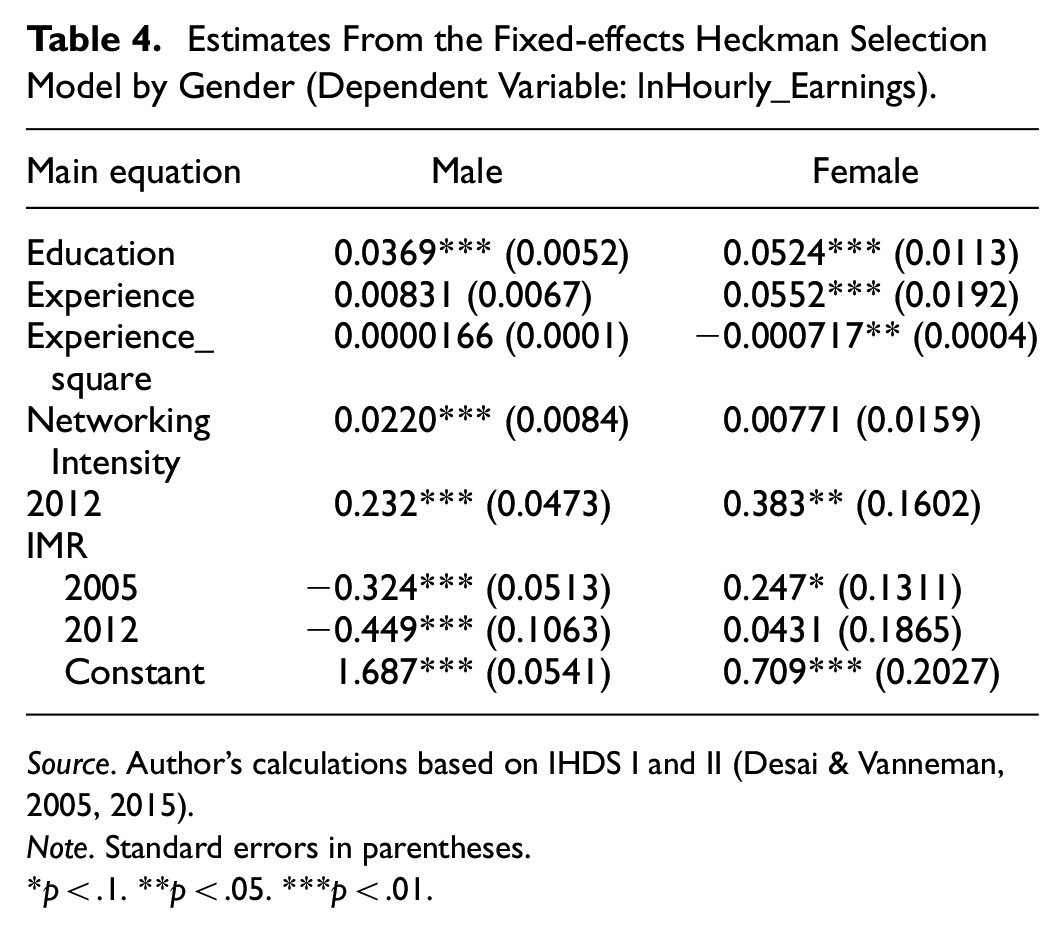
We estimated the model by two groups—male and female—as information was provided for these groups only (see Table 4). Education was positive and significant for both males and females. Experience was positive and significant for females and jointly significant for males. The square term (Experience_square) was negative. This suggests an inverted U-shaped relation between earnings and experience for females. The implication is that while women’s earnings increase with experience, the rate of increase in earning—caused by a rise in experience—occurs at a decreasing rate. Networking intensity was positive and significant for males. The IMR was significant for both groups in 2005 and for males in 2012. Selection equation results are reported in Supplemental Table S6.

Table 4.

Estimates From the Fixed-effects Heckman Selection Model by Gender (Dependent Variable: lnHourly_Earnings).

Main equation	Male	Female
Education	0.0369*** (0.0052)	0.0524*** (0.0113)
Experience	0.00831 (0.0067)	0.0552*** (0.0192)
Experience_square	0.0000166 (0.0001)	−0.000717** (0.0004)
Networking Intensity	0.0220*** (0.0084)	0.00771 (0.0159)
2012	0.232*** (0.0473)	0.383** (0.1602)
IMR
2005	−0.324*** (0.0513)	0.247* (0.1311)
2012	−0.449*** (0.1063)	0.0431 (0.1865)
Constant	1.687*** (0.0541)	0.709*** (0.2027)

Source. Author’s calculations based on IHDS I and II (Desai & Vanneman, 2005, 2015).

Note. Standard errors in parentheses.

*p < .1. **p < .05. ***p < .01.

By Caste

We estimated coefficients for four caste groups (see Table 5). We found that education has a positive and significant impact on all castes except SC. Experience was positive and significant for general castes, OBC, and ST. Experience_square was negative and significant for general, OBC (jointly), and ST. This suggests a U-shaped relation between earnings and experience for the two groups (general and ST). Networking intensity was positive and significant for SC. The IMR was significant for most of the values, indicating the presence of a selection bias. Selection equation results are reported in Supplemental Table S7.

Table 5.

Estimates From the Fixed-effects Heckman Selection Model by Caste (Dependent Variable: lnHourly_Earnings).

Main equation	General	OBC	SC	ST
Education	0.0466*** (0.0000)	0.0191** (0.0448)	0.0599*** (0.0001)	0.0152* (0.0837)
Experience	0.0305*** (0.0020)	−0.00834 (0.4257)	0.0267* (0.0780)	0.00349 (0.7966)
Experience_square	−0.000341** (0.0409)	0.000156 (0.5025)	−0.000249 (0.3933)	−0.0000310 (0.9103)
Networking Intensity	0.0108 (0.2345)	0.0161 (0.2150)	−0.00135 (0.9552)	0.0267 (0.1013)
2012	0.215*** (0.0048)	0.363*** (0.0000)	0.179 (0.2410)	0.374*** (0.0022)
IMR
2005	−0.203*** (0.0013)	−0.186*** (0.0025)	0.0892 (0.4125)	−0.276*** (0.0024)
2012	−0.336*** (0.0002)	−0.341*** (0.0006)	0.0697 (0.7914)	−0.440*** (0.0001)
Constant	1.582*** (0.0000)	1.834*** (0.0000)	1.122*** (0.0000)	1.681*** (0.0000)

Source. Author’s calculations based on IHDS I and II (Desai & Vanneman, 2005, 2015).

Note. Standard errors in parentheses.

p < .1. **p < .05. ***p < .01.

By Religious Groups

Education was significant and positive for all three religious groups (Table 6). Experience, on the other hand, was significant and positive for Hindus but not for the other groups. Networking intensity was significant and positive for Hindus only. Selection equation results are reported in Supplemental Table S8.

Table 6.

Estimates From the Fixed-effects Heckman Selection Model by Religion (Dependent Variable: lnHourly_Earnings).

Main equation	Hindu	Other minorities	Muslim
Education	0.0377*** (0.0049)	0.0998*** (0.0161)	0.0215* (0.0118)
Experience	0.0137** (0.0061)	0.0364* (0.0259)	0.0250 (0.0177)
Experience_square	−0.0000914 (0.0001)	−0.000352 (0.0005)	−0.0000380 (0.0003)
Networking Intensity	0.0223*** (0.0078)	−0.0419 (0.0455)	0.0127 (0.0319)
2012	0.215*** (0.0622)	0.677*** (0.1652)	0.359** (0.1439)
IMR
2005	−0.239*** (0.0509)	0.224** (0.1024)	−0.188* (0.1070)
2012	−0.326*** (0.0751)	−0.631*** (0.1880)	−0.399*** (0.1023)
Constant	1.591*** (0.0616)	1.574*** (0.1877)	1.630*** (0.1853)

Source. Author’s calculations based on IHDS I and II (Desai & Vanneman, 2005, 2015).

Note. Standard errors in parentheses

p < .1. **p < .05. ***p < .01.

Analysis

Our results demonstrate that education is significant and positive for all categories of individuals—economic strata, gender, caste, and religion. However, there is a wide range of returns from education to each of these subgroups.

When we compare returns to education by consumption quintiles (see Figure 1), the values go from 2.4% (BPL) to 8.8% (APL 3). Returns to females (5.2%) are much higher than the returns to males (3.7%).

Figure 1.

Projected earnings by consumption quintile with education and experience as covariates.

The received literature on gender differentials in earnings has universally found that women earn less than men for a given level of education and experience. We did not find evidence contrary to this. However, we did find that there is a tendency toward convergence in earnings between males and females for given levels of education and experience. This has been noted by other authors as well, and it can be attributed to structural and technological change in part (Cortes et al., 2020). As the workforce has moved from manufacturing to service-oriented employment, women are less likely to be disadvantaged in such work situations. Moreover, their soft skills at the workplace may be more sought after than those of men. Our findings provide evidence of convergence in the long run in the Indian context (see Figure 2). We found that the initial value of earnings (intercept value) for males is much higher than that of females. However, the marginal returns to an additional year of education are much higher for women than men.

Figure 2.

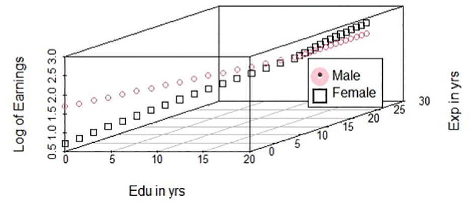
Projected earnings by gender with education and experience as covariates.

Among the caste groups (see Figure 3), the SCs show the highest returns to education (5.9%) followed by the general castes (4.6%). However, general castes have a higher intercept, which elevates their earnings above other castes for almost the entire range of years. Among the religious groups (see Figure 4), Hindus (3.8%) and Muslims (2.3%) have a lower return than other minorities (9.9%). These results suggest that investment in education does pay dividends for social development in India, in alignment with the literature (Tilak, 2021).

Figure 3.

Projected earnings by caste with education and experience as covariates.

Figure 4.

Projected earnings by religion with education and experience as covariates.

There is, therefore, a need for a targeted approach to ensure that these groups do not fall out of the education system for lack of ability to pay (Mishra & Ramakrishna, 2023). The Right of Children to Free and Compulsory Education (RTE) Act of 2009 makes it obligatory for the government to ensure that every child in the age group of 6 to 14 years is provided free and compulsory education (GoI, 2009). This is a step toward inclusive development (Das, 2020) although there is evidence of unintended outcomes (C. Chatterjee et al., 2020). Educational affirmative interventions based on caste and gender have been found to have positive impacts in India (Bagde et al., 2016). Our findings are along the lines of Chakraborty and Bohara’s (2021) study on the role of caste and religion in India and their recommendation for policy intervention for socially backward classes and Muslims to establish equity in the labor market.

There is a constitutionally mandated reservation of jobs in the public sector for less privileged castes (Bhaskar, 2021). This has helped overcome selection bias against the lower castes in the public sector to some extent. However, reservations for women have been limited to the lowest tier of government despite the longstanding proposal to bring in 33% reservations at all tiers of government and in other areas of employment (Marwah, 2019). The presence of women in government has had positive outcomes in local assets and employment creation (Deininger et al., 2020).

Discussion

Currently, three nationwide panel data sets are available at the household level: IHDS, the PLFS, and CPHS. Over two waves at the household level, the IHDS panel data set has been used to study the impact of natural disasters (Tamuly & Mukhopadhyay, 2022) and rural insurance (Azam, 2018). It has also been used at the individual level as a repeated cross-section to study domestic violence (Akter & Chindarkar, 2020) and an individual panel to study women’s health (E. Chatterjee & Sennott, 2021). Sarkar et al. (2019) also use a panel similar to our study but limit themselves to the question of determinants of women’s participation in the labor force in India.

The Government of India also publishes a new data set on employment and unemployment status, PLFS, which is collected every quarter (NSO, 2021). Although the data is collected every quarter, one household is interviewed only once a year, making it a rotational panel. This data has been used by researchers such as Sengupta (2023) to estimate the Mincer equation with a Heckman selection model to predict wages in India. However, some studies have used pooled unit-level data and therefore the estimates are likely to have the limitations that cross-section models encounter, such as omitted variable bias and dynamic relationships among other issues (Hsiao, 2007). We overcome these estimation limitations by using fixed-effect panel data. Our study, therefore, is probably the first study that uses a panel data set to explain the impact of education and experience on earnings in India. While we confirm Sengupta’s (2023) finding that females earn less than men, we add a more nuanced view of the gender gaps in the labor market to the existing literature. We find that while women have lower starting earnings, they have higher incremental earnings as they gain in education and experience. The panel characteristic of the PLFS database has been used to study urban employment in India (Roy et al., 2022). However, it has not been exploited to respond to the question of wage determination.

The other panel data set at the household level currently available is the CPHS. However, the focus of this database is on tracking consumption (Abraham & Shrivastava, 2022) and, similar to the PLFS, it is too short to study medium or long-term impacts on wages attributable to education or experience. Singha Roy (2020) uses a smaller regional panel of 18 villages in semi-arid regions to study wage determination. This study reports that education is significant for men at all levels of education but only significant at the level of graduation for women. A more elaborate study by Khanna (2023) uses a combination of data sets that link individual-level wages to district characteristics to create a district-level panel data set. This study suggests that men gain most from additional years of education than women in terms of wages. We find contrary evidence that even though women start with lower wages than men, their marginal increase for additional years of education and experience out-pace the growth of wages for men.

To our understanding, no study has used a panel data set in the Indian context that has examined the role of education and experience in wage determination with a nationwide representative sample with a household-level panel thus far. Our results, therefore, update all earlier estimates in this context.

In a recent global review, Psacharopoulos and Patrinos (2018) examined 1,120 estimates in 139 countries. They found that the average return from an additional year of education was about 9%. Earlier, Peet et al. (2015) had found the return to education to be about 7.6% in developing countries and this, according to them, was not dissimilar to developed countries. In Indonesia, the impact of school expansion led to an increase in wages by 6.8% to 10.6 % (Duflo, 2001) and returns from higher education were about 15% (Yubilianto, 2020). Most studies indicate heterogeneity in returns by gender and region within and across countries, with a higher return for women and urban workers.

In India, Kingdon and Theopold (2008) used two rounds of NSSO data (1993–1994 and 1999–2000) and found the returns to be 8.2% (1993–1994) and 7.7% (1999–2000) using an OLS regression and similar to estimates of the Heckman model. In a recent study, Bairagya (2020) used the IHDS II data and found the returns to be between 5.6% (OLS) and 9.4% (IV approach). Geetha Rani (2014) found the returns to education to be between 14% (OLS) and 5.1% (Heckman selection model) using the IHDS I data. A gender-disaggregated analysis for an additional year of education result was reported by Fulford (2014), who found private returns to be 9.3% (for males) and (-) 6.5% (for females) using OLS using NSSO data. Mendiratta and Gupt (2013) report the highest returns at 15%, using a pseudo-panel approach with NSSO data for two rounds (2004–2005 and 2009–2010). When returns to education were estimated in a general equilibrium (GE) framework, Khanna (2023) found that skilling led to an increase in returns by 19.9% (without GE effects) and 13.4% (with GE effects).

There seems to be a wide range of variation in the reported private returns to education in India. However, all earlier estimates in the Indian context have used cross-sectional data or a pseudo-panel approach. We improve on all of them by using a nationwide household-level panel, with fixed effects for the Heckman selection model approach. Our results are comparable to some of the international findings on returns to education on average (Hicks & Duan, 2023; Klasen et al., 2021; Korwatanasakul, 2023).

Our study also looked at the role of social capital by examining the impact of networking intensity on different groups. We find that this variable had a positive impact on the earnings of males (among gender groups), Hindus (among religious groups), and APL1 (among consumption quintiles). Our results are in line with the findings of a study based in China (Liu, 2017), where individual-level social capital was found to have a greater impact on men than women. Similar effects were reported by (Smith, 2000) in the context of the United States. Behtoui and Neergaard (2010) found that marginalized groups in Sweden had lower wages on average due to a lack of access to social capital. This could be anticipated in India and might explain the wage gaps for women and marginalized social and religious groups (Deshpande & Khanna, 2021).

Conclusion

Our findings have important policy implications and connect to multiple SDGs, such as poverty (SDG 1), quality education (SDG 4), gender equality (SDG 5), and reduced inequalities (SDG 10). The government of India has been committed to the fulfilment of the SDGs and has undertaken multiple social interventions. In the sphere of education as well, policies have been developed to enhance access and improve quality education. About a decade and a half ago, the Right of Children to Free and Compulsory Education Act or Right to Education Act, 2009, for free and compulsory schooling (GoI, 2009) was enacted to reduce the dropout rate in schools and ensure compulsory education up to 14 years. The New Education Policy announced in 2020 also attempts to upgrade quality education. Our findings provide evidence that education (SDG 4) helps in achieving the goals of gender equality (SDG 5) and social justice for marginalized (caste and religious) groups (SDG 10).

The government has also implemented affirmative action policies in the domain of jobs and education for certain groups based largely on caste (Deshpande, 2013) and, more recently, economic backwardness (Nath, 2019). We find that despite education positively impacting earnings, the less privileged groups would require affirmative action to achieve reduced inequalities (SGD 10) and escape poverty (SGD 1).

Our study addresses the issues of economic distribution, gender, caste, and religion in the context of larger sustainable developmental goals (Dhar, 2018; Pandey, 2019). Our findings of higher marginal returns to education among females justify the need for greater investment in education for women. The lower returns on education among STs and Muslims indicate the need for affirmative action for these groups. Similarly, the positive and significant coefficient for all consumption quintiles suggests that anti-poverty programs in combination with educational opportunities for the less privileged (BPL) would meet the goals of social justice. Development policies that combine multiple objectives would therefore have a more effective welfare outcome.

While several innovations have been implemented in our study, we acknowledge some limitations. We were unable to separate the impact of ability and inherent skills from the years of education in wage determination (ability bias). The reporting of caste was non-uniform in the two rounds of IHDS. This could be due to the re-classification of castes, which was an ongoing process at the time of the survey. This could be further resolved when data from new ongoing survey rounds becomes available. Also, our study did not stratify the labor market by state and sector. Incorporating these classifications could yield new insights in a country like India with large geographic and economic heterogeneity.

Supplemental Material

sj-docx-1-sgo-10.1177_21582440231220942 – Supplemental material for How Much do Education, Experience, and Social Networks Impact Earnings in India? A Panel Data Analysis Disaggregated by Class, Gender, Caste and Religion

Supplemental material, sj-docx-1-sgo-10.1177_21582440231220942 for How Much do Education, Experience, and Social Networks Impact Earnings in India? A Panel Data Analysis Disaggregated by Class, Gender, Caste and Religion by Yasser Razak Hussain and Pranab Mukhopadhyay in SAGE Open

Footnotes

Acknowledgements

We would like to thank five anonymous reviewers of the journal for their comments on an earlier draft. These have helped improve our paper significantly.

Declaration of Conflicting Interests

The author(s) declared no potential conflicts of interest with respect to the research, authorship, and/or publication of this article.

Funding

The author(s) received no financial support for the research, authorship, and/or publication of this article.

Ethical Approval

An ethics statement for animal and human studies is not applicable.

ORCID iDs

Yasser Razak Hussain

Pranab Mukhopadhyay

Data Availability Statement

The data that support the findings of this study are available in the public repository from the Data Sharing for Demographic Research program of ICPSR, the Inter-university Consortium for Political and Social Research: https://www.icpsr.umich.edu/web/DSDR/studies/22626 and

Supplemental Material

Supplemental material for this article is available online.

References

Abraham

Shrivastava

(2022). How comparable are India’s labour market surveys? Indian Journal of Labour Economics, 65(2), 321–346. https://doi.org/10.1007/s41027-022-00381-x

Acemoglu

Autor

(2012). What does human capital do? A review of Goldin and Katz’s: The race between education and technology. Journal of Economic Literature, 50(2), 426–463. https://doi.org/10.1257/jel.50.2.426

Agrawal

(2014). Gender and caste-based wage discrimination in India: Some recent evidence. Journal for Labour Market Research, 47(4), 329–340. https://doi.org/10.1007/s12651-013-0152-z

Akter

Chindarkar

(2020). An empirical examination of sustainability of women’s empowerment using panel data from India. Journal of Development Studies, 56(5), 890–906. https://doi.org/10.1080/00220388.2019.1605054

Angrist

J. D.

Krueger

A. B.

(1991). Does compulsory school attendance affect schooling and earnings? Quarterly Journal of Economics, 106(4), 979–1014. https://doi.org/10.2307/2937954

Angrist

J. D.

Krueger

A. B.

(2001). Instrumental variables and the search for identification: From supply and demand to natural experiments. Journal of Economic Perspectives, 15(4), 69–85. https://doi.org/10.1257/jep.15.4.69

Angrist

Djankov

Goldberg

P. K.

Patrinos

H. A.

(2021). Measuring human capital using global learning data. Nature, 592, 403–408. https://doi.org/10.1038/s41586-021-03323-7

Arabsheibani

Gupta

Mishra

Parhi

(2018). Wage differential between caste groups: Are younger and older cohorts different? Economic Modelling, 74, 10–23. https://doi.org/10.1016/j.econmod.2018.04.019

Ashraf

Q. H.

Weil

D. N.

Wilde

(2013). The effect of fertility reduction on economic growth. Population and Development Review, 39(1), 97–130. https://doi.org/10.1111/j.1728-4457.2013.00575.x

10.

Azam

(2018). Does social health insurance reduce financial burden? Panel data evidence from India. World Development, 102, 1–17. https://doi.org/10.1016/j.worlddev.2017.09.007

11.

Azam

Chin

Prakash

(2013). The returns to English-language skills in India. Economic Development and Cultural Change, 61(2), 335–367. https://doi.org/10.1086/668277

12.

Bagde

Epple

Taylor

(2016). Does affirmative action work? Caste, gender, college quality, and academic success in India. American Economic Review, 106(6), 1495–1521. https://www.jstor.org/stable/43861129

13.

Bairagya

(2020). Returns to education in self-employment in India: A comparison across different selection models (WIDER Working Paper 2020/5). UNU-WIDER. doi: https://doi.org/10.35188/UNU-WIDER/2020/762-0

14.

Baltagi

B. H.

Khanti-Akom

(1990). On efficient estimation with panel data: An empirical comparison of instrumental variables estimators. Journal of Applied Economics, 5(4), 401–406. https://doi.org/10.1002/jae.3950050408

15.

Barro

R. J.

McCleary

R. M.

(2003). Religion and economic growth across countries. American Sociological Review, 68(5), 760–781. https://doi.org/10.2307/1519761

16.

Beam

E. A.

Hyman

Theoharides

(2020). The relative returns to education, experience, and attractiveness for young workers. Economic Development and Cultural Change, 68(2), 391–428. https://doi.org/10.1086/701232

17.

Becker

G. S.

(1962). Investment in human capital: A theoretical analysis. Journal of Political Economy, 70(5, Part 2), 9–49. https://doi.org/10.1086/258724

18.

Becker

G. S.

(Ed.). (1994). Human capital: A theoretical and empirical analysis, with special reference to education (3rd ed.). University of Chicago Press.

19.

Behtoui

Neergaard

(2010). Social capital and wage disadvantages among immigrant workers. Work Employment & Society, 24(4), 761–779. https://doi.org/10.1177/0950017010380640

20.

Bhambhani

Inbanathan

(2018). Not a mother, yet a woman: Exploring experiences of women opting out of motherhood in India. Asian Journal of Women s Studies, 24(2), 159–182. https://doi.org/10.1080/12259276.2018.1462932

21.

Bhaskar

(2021). Reservations, efficiency, and the making of Indian constitution. Economic and Political Weekly, 56(19), 42–49.

22.

Bhattacharya

Sato

(2017). Estimating regional returns to education in India: A fresh look with pseudo-panel data. Progress in Development Studies, 17(4), 282–290. https://doi.org/10.1177/1464993417716357

23.

Bhaumik

S. K.

Chakrabarty

(2008). Does move to market have an impact on earnings gap across gender? Some evidence from India. Applied Economics Letters, 15(8), 601–605. https://doi.org/10.1080/13504850600706651

24.

Bhaumik

S. K.

Chakrabarty

(2010). Earnings inequality in India: Has the rise of caste and religion based politics in India had an impact? In Rakesh

Abusaleh

(Eds.), Handbook of Muslims in India Empirical and Policy Perspectives (pp. 235–253). Oxford University Press.

25.

Blau

F. D.

Gielen

A. C.

Zimmermann

K. F.

(Eds.). (2012). Gender, inequality, and wages (1st ed.). Oxford University Press.

26.

Bound

Jaeger

D. A.

Baker

R. M.

(1995). Problems with instrumental variables estimation when the correlation between the instruments and the endogeneous explanatory variable is weak. Journal of the American Statistical Association, 90(430), 443–450. https://doi.org/10.2307/2291055

27.

Briggs

D. C.

(2004). Causal inference and the Heckman model. Journal of Educational and Behavioral Statistics, 29(4), 397–420. https://doi.org/10.3102/10769986029004397

28.

Card

(1999). The causal effect of education on earnings. Handbook of Labor Economics, 3a, 1801–1863. https://doi.org/10.1016/S1573-4463(99)03011-4

29.

Carneiro

Heckman

J. J.

Vytlacil

(2011). Estimating marginal returns to education. American Economic Review, 101(6), 2754–2781. https://doi.org/10.1257/aer.101.6.2754

30.

Chakraborty

Bohara

A. K.

(2021). The cost of being ‘backward’ in India: Socio-religious discrimination in the labour market. Indian Journal of Human Development, 15(2), 252–274. https://doi.org/10.1177/09737030211029634

31.

Chakraborty

Bohara

A. K.

Binder

Santos

(2020). Is the Indian labor market biased against women? In Jivetti

Hoque

(Eds.), Population Change and Public Policy (pp. 229–242). Springer International Publishing.

32.

Chatterjee

Hanushek

E. A.

Mahendiran

(2020). Can greater access to education be inequitable? New evidence from India’s Right to Education Act (Working Paper No. 27377). National Bureau of Economic Research. doi: https://doi.org/10.3386/w27377

33.

Chatterjee

Sennott

(2021). Fertility intentions and child health in India: Women’s use of health services, breastfeeding, and official birth documentation following an unwanted birth. PLoS One, 16(11), 1–12. https://doi.org/10.1371/journal.pone.0259311

34.

Chun

(2002). An instrumental variable estimate of the effect of fertility on the labour force participation of married women. Applied Economics Letters, 9(10), 631–634. https://doi.org/10.1080/13504850110117850

35.

Collin

Weil

D. N.

(2020). The effect of increasing human capital investment on economic growth and poverty: A simulation exercise. Journal of Human Capital, 14(1), 43–83. https://doi.org/10.1086/708195

36.

Comola

de Mello

(2013). Salaried employment and earnings in Indonesia: New evidence on the selection bias. Applied Economics, 45(19), 2808–2816. https://doi.org/10.1080/00036846.2012.667551

37.

Cortes

G. M.

Oliveira

Salomons

(2020). Do technological advances reduce the gender wage gap? Oxford Review of Economic Policy, 36(4), 903–924. https://doi.org/10.1093/oxrep/graa051

38.

Cruz

L. M.

Moreira

M. J.

(2005). On the validity of econometric techniques with weak instruments inference on returns to education using compulsory school attendance laws. Journal of Human Resources, 40(2), 393–410. https://doi.org/10.3368/jhr.XL.2.393

39.

Das

(2020). Understanding equity through Section 12(1)(c) of the Right to Education Act in India. Cambridge Educational Research e-Journal, 7, 53–69. https://doi.org/10.17863/CAM.58327

40.

Dasgupta

(2005). Economics of social capital. Economic Record, 81(s1), S2–S21. https://doi.org/10.1111/j.1475-4932.2005.00245.x

41.

Deaton

(1985). Panel data from time series of cross-sections. Journal of Econometrics, 30(1–2), 109–126. https://doi.org/10.1016/0304-4076(85)90134-4

42.

Deininger

Nagarajan

H. K.

Singh

S. K.

(2020). Women’s political leadership and economic empowerment: Evidence from public works in India. Journal of Comparative Economics, 48(2), 277–291. https://doi.org/10.1016/j.jce.2019.12.003

43.

Desai

Vanneman

(2005). India Human Development Survey (IHDS), 2005. Inter-University Consortium for Political and Social Research. doi: https://doi.org/10.3886/ICPSR22626.v12

44.

Desai

Vanneman

(2015). India Human Development Survey-II (IHDS-II), 2011-12. Inter-University Consortium for Political and Social Research. doi: https://doi.org/10.3886/ICPSR36151.v6

45.

Deshpande

(2011). The grammar of caste: Economic discrimination in contemporary India. Oxford University Press.

46.

Deshpande

(2013). Social justice through affirmative action in India: An assessment. In Wicks-Lim

Pollin

(Eds.), Capitalism on trial (pp. 266–287). Edward Elgar Publishing.

47.

Deshpande

Khanna

(2021). Can weak ties create social capital? Evidence from self-help groups in rural India. World Development, 146, 1–20. https://doi.org/10.1016/j.worlddev.2021.105534

48.

Dhar

(2018). Gender and sustainable development goals (SDGs). Indian Journal of Gender Studies, 25(1), 47–78. https://doi.org/10.1177/0971521517738451

49.

Dhesi

A. S.

Singh

(1989). Education, labour market distortions and relative earnings of different religion-caste categories in India (A case study of Delhi). Canadian Journal of Development Studies, 10(1), 75–89. https://doi.org/10.1080/02255189.1989.9669352

50.

Duflo

(2001). Schooling and labor market consequences of school construction in Indonesia: Evidence from an unusual policy experiment. American Economic Review, 91(4), 795–813. https://doi.org/10.1257/aer.91.4.795

51.

Eisnecker

P. S.

Adriaans

(2023). How do my earnings compare? Pay referents and just earnings. European Sociological Review, 1–14. https://doi.org/10.1093/esr/jcad002

52.

England

Folbre

(2023). Reconceptualizing human capital. In Tåhlin

(Ed.), A research agenda for skills and inequality (pp. 177–195). Edward Elgar Publishing.

53.

Faggian

Modrego

McCann

(2019). Human capital and regional development. In Capello

Nijkamp

(Eds.), Handbook of regional growth and development theories (pp. 149–171). Edward Elgar Publishing.

54.

Fulford

(2014). Returns to education in India. World Development, 59(C), 434–450. https://doi.org/10.1016/j.worlddev.2014.02.005

55.

Geetha Rani

(2013). Exploring earnings and education disparities in India across region, caste, religion and English language ability. Artha Vijnana, 55(4), 402–420. https://doi.org/10.21648/arthavij/2013/v55/i4/111243

56.

Geetha Rani

(2014). Disparities in earnings and education in India. Cogent Economics & Finance, 2(1), 1–18. https://doi.org/10.1080/23322039.2014.941510

57.

GoI. (2006). Social, economic and educational status of the Muslim community of India: A report. Prime Minister’s High Level Committee, Cabinet Secretariat, Government of India. https://www.education.gov.in/sites/upload_files/mhrd/files/sachar_comm.pdf

58.

GoI. (2009). The Right of Children to Free and Compulsory Education (RTE) Act, 2009. Government of India. https://www.education.gov.in/sites/upload_files/mhrd/files/upload_document/rte.pdf

59.

GoI. (2016). National commission for scheduled castes handbook-2016. National Commission for Scheduled Castes, Government of India.

60.

Goldin

(2016). Human capital. In Diebolt

Haupert

(Eds.), Handbook of cliometrics (pp. 55–86). Springer.

61.

Harmon

Walker

Westergård-Nielsen

N. C.

(Eds.) (2001). Education and earnings in Europe: A cross country analysis of the returns to education. Edward Elgar Publishing.

62.

Hartog

Gerritsen

(2016). Mincer earnings functions for the Netherlands 1962–2012. De Economist, 164(3), 235–253. https://doi.org/10.1007/s10645-016-9279-y

63.

Heckman

(1974). Shadow prices, market wages, and labor supply. Econometrica, 42(4), 679–694. https://doi.org/10.2307/1913937

64.

Heckman

J. J.

(1976). The common structure of statistical models of truncation, sample selection and limited dependent variables and a simple estimator for such models. Annals of Economic and Social Measurement, 5(4), 475–492.

65.

Heckman

J. J.

(1979). Sample selection bias as a specification error. Econometrica, 47(1), 153–161. https://doi.org/10.2307/1912352

66.

Heckman

J. J.

Lochner

L. J.

Todd

P. E.

(2006). Earnings functions, rates of return and treatment effects: The Mincer equation and beyond. In Hanushek

Welch

(Eds.), Handbook of the economics of education (Vol. 1, pp. 307–458). Elsevier.

67.

Heckman

Polachek

(1974). Empirical evidence on the functional form of the earnings-schooling relationship. Journal of the American Statistical Association, 69(346), 350–354. https://doi.org/10.1080/01621459.1974.10482952

68.

Hicks

Duan

(2023). Education as opportunity? The causal effect of education on labor market outcomes in Jordan. Oxford Development Studies, 51(2), 179–197. https://doi.org/10.1080/13600818.2023.2177264

69.

Hoffmann

Kassouf

A. L.

(2005). Deriving conditional and unconditional marginal effects in log earnings equations estimated by Heckman’s procedure. Applied Economics, 37(11), 1303–1311. https://doi.org/10.1080/00036840500118614

70.

Hsiao

(2007). Panel data analysis—Advantages and challenges. Test, 16(1), 1–22. https://doi.org/10.1007/s11749-007-0046-x

71.

Jacob

J. F.

(2018). Higher education in India from 1983 to 2014: Participation, access and labour market outcomes across socio-religious groups. Indian Journal of Human Development, 12(1), 74–92. https://doi.org/10.1177/0973703018777180

72.

Jaumotte

(2003). Female labour force participation: Past trends and main determinants in OECD countries (OECD Working Paper No. 376). doi: http://dx.doi.org/10.1787/082872464507

73.

Kamhöfer

D. A.

Schmitz

(2016). Reanalyzing zero returns to education in Germany. Journal of Applied Economics, 31(5), 912–919. https://doi.org/10.1002/jae.2461

74.

Khanna

(2023). Large-scale education reform in general equilibrium: Regression discontinuity evidence from India. Journal of Political Economy, 131, 549–591. https://doi.org/10.1086/721619

75.

Kingdon

G. G.

Theopold

(2008). Do returns to education matter to schooling participation? Evidence from India. Education Economics, 16(4), 329–350. https://doi.org/10.1080/09645290802312453

76.

Klasen

T. T. N.

Pieters

Santos Silva

(2021). What drives female labour force participation? Comparable micro-level evidence from eight developing and emerging economies. Journal of Development Studies, 57(3), 417–442. https://doi.org/10.1080/00220388.2020.1790533

77.

Korwatanasakul

(2023). Returns to schooling in Thailand: Evidence from the 1978 compulsory schooling law. Developing Economies, 61(1), 3–35. https://doi.org/10.1111/deve.12341

78.

Kugler

A. D.

Kumar

(2017). Preference for boys, family size, and educational attainment in India. Demography, 54(3), 835–859. https://doi.org/10.1007/s13524-017-0575-1

79.

Kumar

Hashmi

N. I.

(2020). Labour market discrimination in India. Indian Journal of Labour Economics, 63(1), 177–188. https://doi.org/10.1007/s41027-019-00203-7

80.

Leigh

(2008). Returns to education in Australia. Economic Papers, 27(3), 233–249. https://doi.org/10.1111/j.1759-3441.2008.tb01040.x

81.

Lemieux

(2006). The “Mincer equation” thirty years after schooling, experience, and earnings. In Grossbard

(Ed.), Jacob Mincer A pioneer of modern labor economics (pp. 127–145). Springer.

82.

(2003). Economic transition and returns to education in China. Economics of Education Review, 22(3), 317–328. https://doi.org/10.1016/s0272-7757(02)00056-0

83.

Liu

(2017). Role of individual social capital in wage determination: Evidence from China. Asian Economic Journal, 31(3), 239–252. https://doi.org/10.1111/asej.12122

84.

Lolayekar

A. P.

Mukhopadhyay

(2020). Understanding growth convergence in India (1981-2010): Looking beyond the usual suspects. PLoS One, 15(6), 1–17. https://doi.org/10.1371/journal.pone.0233549

85.

Madheswaran

Singhari

(2016). Social exclusion and caste discrimination in public and private sectors in India: A decomposition analysis. Indian Journal of Labour Economics, 59(2), 175–201. https://doi.org/10.1007/s41027-017-0053-8

86.

Mamgain

R. P.

(2021). Understanding labour market disruptions and job losses amidst COVID-19. Journal of Social and Economic Development, 23(Suppl 2), 301–319. https://doi.org/10.1007/s40847-020-00125-x

87.

Marwah

(2019). Gender, caste and Indian feminism the case of the Women’s Reservation Bill. In Aneja

(Ed.), Women’s and gender studies in India: Crossings (pp. 1–13). Routledge India.

88.

Mehrotra

(2019). Informal employment trends in the Indian economy: Persistent informality, but growing positive development (Working Paper No. 254). International Labour Organization. https://www.ilo.org/employment/Whatwedo/Publications/working-papers/WCMS_734503/lang–en/index.htm

89.

Mendiratta

Gupt

(2013). Private returns to education in India by gender and location: A pseudo-panel approach. Arthaniti-Journal of Economic Theory and Practice, 12(1-2), 48–69. https://doi.org/10.1177/0976747920130103

90.

Mincer

(1958). Investment in human capital and personal income distribution. Journal of Political Economy, 66(4), 281–302. https://doi.org/10.1086/258055

91.

Mincer

(1974). Schooling, experience, and earnings. National Bureau of Economic Research. http://www.nber.org/books/minc74-1

92.

Mishra

Ramakrishna

(Eds.) (2023). Education of socio-economic disadvantaged groups: From marginalisation to inclusion. Routledge India.

93.

Mitra

(2019). Returns to education in India: Capturing the heterogeneity. Asia & the Pacific Policy Studies, 6(2), 151–169. https://doi.org/10.1002/app5.271

94.

Mohanty

(2021). A distributional analysis of the gender wage gap among technical degree and diploma holders in urban India. International Journal of Educational Development, 80, 1–16. https://doi.org/10.1016/j.ijedudev.2020.102322

95.

Mosse

(2018). Caste and development: Contemporary perspectives on a structure of discrimination and advantage. World Development, 110, 422–436. https://doi.org/10.1016/j.worlddev.2018.06.003

96.

Mroz

T. A.

(1987). The sensitivity of an empirical model of married women’s hours of work to economic and statistical assumptions. Econometrica, 55(4), 765–799. https://doi.org/10.2307/1911029

97.

Mundlak

(1978). On the pooling of time series and cross section data. Econometrica, 46(1), 69–85. https://doi.org/10.2307/1913646

98.

Nath

(2019). Employment scenario and the reservation policy. Economic and Political Weekly, 54(19), 56–61.

99.

NSO. (2021). Annual Report Periodic Labour Force Survey (PLFS) (July 2019 - June 2020). National Statistical Office, Ministry of Statistics and Programme Implementation, Government of India. https://www.mospi.gov.in/sites/default/files/publication_reports/Annual_Report_PLFS_2019_20F1.pdf

100.

Pandey

(2019). Ensure quality education for all in India: Prerequisite for achieving SDG 4. In Chaturvedi

James

T. C.

Saha

Shaw

(Eds.), 2030 Agenda and India: Moving from quantity to quality (pp. 165–196). Springer.

101.

Patrinos

(2016). Estimating the return to schooling using the Mincer equation. IZA World of Labor, 278, 1–11. https://doi.org/10.15185/izawol.278

102.

Patrinos

H. A.

Psacharopoulos

(2020). Returns to education in developing countries. In Bradley

Green

(Eds.), The economics of education (2nd ed., pp. 53–64). Academic Press.

103.

Peet

E. D.

Fink

Fawzi

(2015). Returns to education in developing countries: Evidence from the living standards and measurement study surveys. Economics of Education Review, 49, 69–90. https://doi.org/10.1016/j.econedurev.2015.08.002

104.

Polachek

S. W.

(2008). Earnings over the life cycle: The Mincer earnings function and its applications. Foundations and Trends in Microeconomics, 4(3), 165–272. https://doi.org/10.1561/0700000018

105.

Psacharopoulos

Patrinos

H. A.

(2018). Returns to investment in education: A decennial review of the global literature. Education Economics, 26(5), 445–458. https://doi.org/10.1080/09645292.2018.1484426

106.

Ray

Katzenstein

M. F.

(2005). Social movements in India: Poverty, power, and politics. Rowman & Littlefield.

107.

Rios-Avila

(2021). XTHECKMANFE: Stata module to fit panel data models in the presence of endogeneity and selection. Statistical Software Components S458770. Boston College Department of Economics. https://ideas.repec.org/c/boc/bocode/s458770.html

108.

Rossi

P. E.

(2014). Invited paper—Even the rich can make themselves poor: A critical examination of IV methods in marketing applications. Marketing Science, 33(5), 655–672. https://doi.org/10.1287/mksc.2014.0860

109.

Roy

Saroj

Pradhan

(2022). Nature of employment and outcomes for urban labor: Evidence from the latest labor force surveys in India. Indian Economic Review, 57(1), 165–221. https://doi.org/10.1007/s41775-022-00131-2

110.

Sarkar

Sahoo

Klasen

(2019). Employment transitions of women in India: A panel analysis. World Development, 115, 291–309. https://doi.org/10.1016/j.worlddev.2018.12.003

111.

Schultz

T. W.

(1961). Investment in human capital. American Economic Review, 51(1), 1–17.

112.

Schwiebert

(2012). Revisiting the composition of the female workforce: A Heckman selection model with endogeneity (Hannover Economic Papers (HEP) DP-502). University of Leibniz.

113.

Semykina

Wooldridge

J. M.

(2010). Estimating panel data models in the presence of endogeneity and selection. Journal of Econometrics, 157(2), 375–380. https://doi.org/10.1016/j.jeconom.2010.03.039

114.

Sen

(2000). Development as freedom. Anchor Books.

115.

Sen

(2001). Economic development and capability expansion in historical perspective. Pacific Economic Review, 6(2), 179–191. https://doi.org/10.1111/1468-0106.00126

116.

Sengupta

(2023). Effect of COVID-19 pandemic on employment and earning in urban India during the first three months of pandemic period: An analysis with unit-level data of periodic labour force survey. Indian Journal of Labour Economics, 66(1), 283–298. https://doi.org/10.1007/s41027-023-00428-7

117.

Sengupta

Das

(2014). Gender wage discrimination across social and religious groups in India: Estimates with unit level data. Economic and Political Weekly, 49(21), 71–76.

118.

Singha Roy

(2020). Wage rate: Is this return to education or return to physical capability? Evidence from rural India. Indian Journal of Labour Economics, 63(1), 99–117. https://doi.org/10.1007/s41027-020-00205-w

119.

Smith

S. S.

(2000). Mobilizing social resources: Race, ethnic, and gender differences in social capital and persisting wage inequalities. Sociological Quarterly, 41(4), 509–537. https://doi.org/10.1111/j.1533-8525.2000.tb00071.x

120.

Tamuly

Mukhopadhyay

(2022). Natural disasters and well-being in India: A household-level panel data analysis. International Journal of Disaster Risk Reduction, 79, 1–14. https://doi.org/10.1016/j.ijdrr.2022.103158

121.

The World Bank. (n.d). World development indicators. https://datacatalog.worldbank.org/dataset/world-development-indicators

122.

Tilak

J. B. G.

(Ed.) (2021). Education in India: Policy and practice. Sage Publications India Pvt Ltd.

123.

Truong

T. H.

Ogawa

Sanfo

J.-B. M. B.

(2021). Educational expansion and the economic value of education in Vietnam: An instrument-free analysis. International Journal of Educational Research, 2, 1–10. https://doi.org/10.1016/j.ijedro.2020.100025

124.

Vasudeva Dutta

(2006). Returns to education: New evidence for India, 1983–1999. Education Economics, 14(4), 431–451. https://doi.org/10.1080/09645290600854128

125.

Wooldridge

J. M.

(Ed.). (2018). Introductory econometrics: A modern approach (7th ed.). Cengage Learning.

126.

Yubilianto. (2020). Return to education and financial value of investment in higher education in Indonesia. Journal of Economic Structures, 9(1), 17. https://doi.org/10.1186/s40008-020-00193-6

Supplementary Material

Please find the following supplemental material available below.

For Open Access articles published under a Creative Commons License, all supplemental material carries the same license as the article it is associated with.

For non-Open Access articles published, all supplemental material carries a non-exclusive license, and permission requests for re-use of supplemental material or any part of supplemental material shall be sent directly to the copyright owner as specified in the copyright notice associated with the article.

0.00 MB

0.08 MB

How Much do Education,Experience,and Social Networks Impact Earnings in India? A Panel Data Analysis Disaggregated by Class,Gender,Caste and Religion

Abstract

Plain Language Summary

Keywords

Introduction

Literature Review

Material and Methods

Data

Sub-Sample Selection

Variables

Empirical Model

Econometric Models, Estimation, and Tests

Results

By Consumption Quintiles

By Gender

By Caste

By Religious Groups

Analysis

Discussion

Conclusion

Supplemental Material

sj-docx-1-sgo-10.1177_21582440231220942 – Supplemental material for How Much do Education, Experience, and Social Networks Impact Earnings in India? A Panel Data Analysis Disaggregated by Class, Gender, Caste and Religion

Footnotes

Acknowledgements

Declaration of Conflicting Interests

Funding

Ethical Approval

ORCID iDs

Data Availability Statement

Supplemental Material

References

Supplementary Material