
Abstract
The structure and functions of neighborhoods determine the impact of measures used to estimate the distribution of street robbery across space and time. The risk of street robbery could vary between different sections of the area. Prior research has typically relied on one-dimensional analysis, which sparsely accounts for the hierarchical configuration of a neighborhood’s influence on spatial crime distribution. Much less is known about how the predictor variables moderate each other at different neighborhood levels. Data was collected from 13,789 US Census blocks (N = 13,788) aggregated to administrative neighborhoods (N = 278) to examine how neighborhood structure affects street robbery distribution at two spatial levels. A Risk Terrain Model was adopted to develop a physical environment risk measure—Aggregate Neighborhood Risk of Crime (ANROC), which, alongside sociodemographic risk factors, predicted the outcomes of the Negative Binomial General Linear Regression models. Study findings suggest that individual-level (block) and group (neighborhood) level predictors influenced street robbery. Both group-level physical environment and total population moderated the impact of the individual-level physical environment on street robbery incidents.
Plain Language Summary
How neighborhoods are structured and function influences the places and the times that street robberies occur. This means that the risk of street robbery will differ between neighborhoods, just as it will be different between different places within the same neighborhood. This research examined the effect of physical environment facilities (ANROC) and social forces, such as the proportion of single-female-headed homes, the population under 18 years, and the proportion of renters on street robbery. It examined the different levels of street robbery between 278 neighborhoods in the City of Baltimore, Maryland. The study also examined the differences in the levels of street robbery between the 13,789 places (blocks) within the neighborhoods. The study found that the forces determined by the places within and between the neighborhoods influenced the distribution of street robbery. Notably, the physical environment forces (ANROC) and the total population of the neighborhoods moderated how the physical environment influenced street robbery at places within the neighborhoods.
Keywords
Introduction
The present study combines Risk Terrain (RTM) and Multilevel (MLM) models to examine the spatial patterns of street robbery predicted by the physical environment and sociodemographic factors. RTM-based measures of the physical environment and sociodemographic forces continue to generate critical interest in diverse aspects of crime pattern research (Andresen & Hodgkinson, 2018; Caplan & Kennedy, 2016; Drucker, 2011). Furthermore, crime pattern research explores the homogeneity of risk factors across neighborhoods within a city. Therefore, it is pertinent to examine the impact of hierarchies of neighborhoods on the moderation of crime distribution by sociodemographic forces and the physical environment (Brantingham et al., 2009; Burgason et al., 2014; Sampson et al., 1997).
Neighborhood measures of risk and their interaction are essential elements for capturing the multidimensional effects of the predictor variables of crimes like street robbery over time and space since the structure and functions of the neighborhoods determine the influence of these variables on crime (Andresen et al., 2017; Bernasco & Block, 2011; Braga et al., 2009). However, most spatial studies of crime distribution do not directly account for variations in within-group versus between-group risk-factor effects among the city-delineated neighborhoods. As suggested by Allen (2005), settings incorporating multiple geographic and structural communities should clarify issues related to levels of analysis. The inattention to nested data often results in inaccurate estimations (Allen, 2005). Previous research examining risk factors that impact crime distribution has commonly relied on individual-level factors to explain group-level occurrences (Drawve & Barnum, 2018; Gerell, 2018).
The present analysis focused on Baltimore City, Maryland’s capital and principal city area. Baltimore has consistently ranked as one of the most dangerous cities in the United States. According to the Federal Bureau of Investigation, the violent crime rate in Baltimore is 2,027 for every 100,000 people (U.S. DOJ FBI, 2017). In addition, the City has identified Robbery and Assault offenses as significant problems (Esquivel et al., 2020). In a 2021 city-wide plan to prevent violence in Baltimore submitted by Mayor Brandon Scott, the City of Baltimore relived the city government’s frustration and strategies for evaluating and engaging the community to prevent violent Crime (Scott, 2021). However, the problem of understanding the distribution, causes, procedures, and policies for containing violent crimes in Baltimore neighborhoods persists. Among violent crimes, street robbery is a significant headache for the administrators of criminal justice in the City. Not much research has systematically examined the prediction of street robbery in the city area by considering individual spatial micro units in group-level neighborhoods. The neighborhood characteristics influence micro-level responses to the predictors of Crime (Burgason et al., 2014). The study conducted a risk terrain modeling of risk factors of street robbery events combined into a single built environment risk factor—Aggregate Neighborhood Risk of Crime (ANROC). Based on the resulting RTM risk measure, the study uses a hierarchical linear model to predict the impact of the physical environment in the presence of sociodemographic forces on street robbery incidents. The following sections explain the background concepts, methodology, and results. The discussion and conclusions follow after that with implications for policy and research.
Predictors of Street Robbery and the Structural Neighborhood
Three criminological theoretical approaches are critical to merging these study’s primary elements—social disorganization, crime pattern (CPT), and routine activities (RAT) theories. Social disorganization theorists contend that the confluence of poverty, racial/ethnic composition, family structure and dependence, residential mobility, and home ownership structure affect crime rate as they diminish social efficacy and the weld of within-group community associations and responsibility. The theory asserts that community structure and characteristics determine crime (Sampson et al., 1997; Shaw & McKay, 1942). The flight of residence from the increased crime rate increases neighborhood poverty and enables racial transition (Borgess & Hipp, 2010). On the spatial angle, crime pattern theorists describe the role of place on the activities of offenders and victims and how crime could emerge at the convergence of both activity spaces (Brantingham & Brantingham, 1993b, 1995).
On the other hand, RAT explains that a triad of elements is required for a crime to occur. These elements are a motivated offender, a lucrative target, and a lack of guardianship (Cohen & Felson, 1979; Roncek & Maier, 1991). Thus connected to crime pattern theory, RAT exemplifies the critical role of opportunism in that the places where those elements meet to increase the likelihood of Crime (Cornish & Clarke, 1987).
Local community and state administrative systems define neighborhoods for effective governance, crime prevention, and intervention. For instance, there are officially 278 geographically designated organic neighborhoods beyond the level of neighborhood blocks in the City of Baltimore (Kent & Karner, 2019). U.S. Census enumerated statistics are captured at different levels below and above these organic neighborhoods, each of whose functioning can be related to its within-group spaces. It is essential, therefore, to account for how the structure of neighborhoods at different structural levels impacts the stability, risk, and contextual forces of crime distribution. These processes form the group and individual effects. On the socio-spatial dimension, residential mobility variables have been, over time, related to crime distribution (Bernasco et al., 2017; Ejiogu, 2020; Haberman & Ratcliffe, 2015). Borgess and Hipp (2010) argue that the racial/ethnic context of crime may affect residential mobility. The residential mobility variable is a proxy for the proportion of renters compared to homeowners, which measures the stability of neighborhood social efficacy (Ejiogu, 2020; Haberman & Ratcliffe, 2015). Residential stability positively affects crime rates (Kasarda & Janowitz, 1974; Sampson & Groves, 1989). Racial heterogeneity is another critical sociodemographic risk variable influencing crime concentration across space (Ejiogu, 2020; Haberman & Ratcliffe, 2015). As observed by numerous studies (Bernasco et al., 2017; Ejiogu, 2020; Haberman & Ratcliffe, 2015), neighborhoods with a high proportion of minority residents being vulnerable to crime points to a downward trend in residential stability (Borgess & Hipp, 2010). Additionally, the proportion of single-parent-headed households is another neighborhood structural factor that diminishes the resident’s collegiate efforts to act and control crime and delinquency (Borgess & Hipp, 2010). The functions of the neighborhood’s risk factors first manifest in the loss of social efficacy (Sampson et al., 1997). They diminish neighborhood structural cohesion, the control of incivilities, and cooperate supervision (Brantingham & Brantingham, 1993b). For instance, high racial heterogeneity has positively influenced violent crimes (Smith et al., 2000) and street robberies (Haberman & Ratcliffe, 2015). However, studies have also reported opposite results (Ejiogu, 2020). This situation suggests that the structure of communities and neighborhoods may have unique determining functions requiring individual analysis to sort and understand. Moreover, the context in which the relationship between these structural factors and crime occurs matters (Borgess & Hipp, 2010).
For instance, the stability of residents in poor and socially disorganized neighborhoods may be related to financial incapacitation to move than a form of social efficacy (Warner & Pierce, 1993, cited in Borgess & Hipp, 2010).Hipp’s (2007) suggested that while it is essential to consider theoretical concepts that provide clues appropriate at levels of aggregation for crime distribution studies, neighborhoods can more or less derive from many dimensions and levels. However, how individual variables moderate crime events at different levels of a neighborhood structure has been sparsely studied (Thomas et al., 2020).
RTM and ANROC Measure of the Physical Environment
Risk terrain modeling (RTM) uses the physical environment and sociodemographic contextual factors to predict the potential of crime events at particular locations (Caplan & Kennedy, 2016). RTM is a theoretical density and proximity spatial analysis that correlates the risk factors to the location of crime concentration. It incorporates and tests the ideas of—crime place theorists, such as the foundational ideas of crime attractors and generators by Brantingham and Brantingham (1993a). The Risk Terrain Modeling Diagnostic (RTMDx) comprises aggravating and protective models used to identify the factors that increase and decrease crime, respectively (Caplan & Kennedy, 2016; Caplan et al., 2013). The basis of operationalizing the distance relationships between the risk factors and the crime outcome is the presence of the predictor within an actual distance of the crime event. Similarly, the concentration of the predictors within an actual distance of the crime incident forms the basis for operationalizing density. The basis of the risk terrain model is the place-crime theory’s assumption that physical geography and sociodemographic risk factors have defined spatial spheres of influence (Caplan & Kennedy, 2016; Caplan et al., 2013). The tool is applied for strategic and tactical deployment to predict crime-vulnerable places, identify risk factors, mitigate, and develop interventions (Caplan & Kennedy, 2016; Caplan et al., 2013). However, the strength of the RTMDx algorithm is that it factors theoretically placed based crime—risk associations to allot weights to the environmental and associated contextual risk factors. In the RTM analysis, the crime predictors (factors) are points in space overlaid by spatial square grids using the kernel density or kernel proximity process to estimate the spatial influence of the risk factors (Caplan & Kennedy, 2016).
In a meta-analysis of 25 studies selected through a systematic review process, Marchment and Gill (2021) found that risk terrain modeling has a proven effect in predicting areas that are prone to high-risk events for driving under the influence (DWI), violent crimes, drug-related crimes, terrorism, and child maltreatment. Robbery studies consistently had higher RTM predictive accuracy ratings than other acquisitive crime types. In addition, studies have adopted the risk terrain modeling process to understand and develop interventions for mitigating robbery (Dugato, 2013) and predict crime distribution due to physical and social risk factors (Garnier et al., 2018). The RTM has been effectively used to predict areas with the most significant risks of violent crimes (Anyinam, 2015) and to develop ANROC composed of diverse physical and contextual risk factors (Drawve et al., 2016). This analytic approach is for understanding diverse modes of violent Crime (Giminez-Santana et al., 2018), including exposure to assault and homicide (Kennedy et al., 2016; Valasik, 2018; Valasik et al., 2019), and terrorism (Marchment et al., 2020). ANROC is a measure determined by the spatial aggregation of multiple RTM-determined risk factors. ANROC captures the neighborhood risk associated with the physical environment (Thomas et al., 2020).
Multilevel Modeling
Multilevel models consider community-level causes of crime at the place or micro levels—just like examining the individual-level outcome from relations between the individual and societal structure. Indeed it exemplifies the issue of community-level variations in crime causation and prevention (Taylor, 2010) by examining the impact of individual-level or community-level features or characteristics on individual outcomes. Spatial communities within neighborhoods include street-level blocks. Taylor notes that depending on the determining theory, community-level features include demographic structural dimensions, land use features, crime rate, and social, cultural, or political climate. Understanding the conceptual linkages between crime causation, crime place, crime opportunity theories, and multilevel models begins with the factors influencing individual-level outcomes. These include the effect of community-level characteristics on individual-level attributes and the impact of individual-level characteristics on individual-level outcomes. In other words, community or neighborhood-level (macro) contexts shape individual-level (micro) dynamics (Taylor, 2010). The significance of the multilevel model is that it allows us to track variation in the outcome due to characteristics within and between the communities. It also allows us to track the variation in the effect of the individual predictors across the communities and the sampling error portion between community variations. Additionally, the multilevel model provides functions to track cross-level interaction—that is, the influence of community or neighborhood characteristics on the impact of the individual predictor. Similarly, it is also feasible to examine the covariation of parameters such as slopes and intercepts of the community characteristics (Taylor, 2010).
In multilevel theoretical modeling combining RAT and social disorganization theories, street (micro) and neighborhood level effect of criminogenic variables was tested on the count of crimes—such as on violent and property crimes—to understand the connection between the two levels of neighborhoods (Jones & Pridemore, 2019). Using a negative binomial regression and controlling for spatial dependence, Jones and Pridemore (2019) showed that both micro and neighborhood-level variables affected street segment violent and property crime. Cross-level interaction tests showed that neighborhood-level characteristics moderated the relationship between micro-level variables and crime and improved the regression models’ explanatory power. Deryol et al. (2016) also examined the multilevel theory of crime places—nodes, paths, and environmental backcloth, using a Poisson regression test. They examined variation in the place-level crime count based on the proximity distance from crime-attracting facilities such as liquor establishments, closest liquor carry-out facilities, and closest bus routes. They configured macro-neighborhood level context as characteristics of census blocks, such as the density of commercial places. The three-way interaction effect of the distances from the crime incident address to the crime-attracting places varied across the neighborhoods—and had a strong negative influence on crime within high commercial density neighborhoods.
The results suggest additional crime prevention intervention for places with numerous nodes and paths to crime-attracting places within the macro neighborhood with dense commercial activities. Velez (2001) conducted a multilevel analysis of victimization risk examining the role of public social control in urban neighborhoods. Individual household victimization characteristics served as micro-level variables, while the level of public social control across 60 urban neighborhoods served as the macro-level characteristics. Valez (2001) found that neighborhoods with public social control reduce the likelihood of individual victimization.
This result suggests that with high levels of public social controls, residents would likely be less prone to victimization, especially in disadvantaged neighborhoods. Tseloni (2006) examined repeat property victimizations based on the 2000 British crime survey and 1991 area statistics by estimating a random effects multilevel model of the household as micro-level units and designated areas as community-level units. The negative binomial regression test results indicated that household, area, and interaction effects explained significant variation in property crimes. The results also showed significant covariation and random variance of the household characteristics between the area units. For instance, single-parent households interacted and enhanced the impact of households involved in neighborhood watch programs on property crimes. While belonging to a neighborhood watch program decreased the count of burglaries and thefts, single-parent households significantly increased burglaries and thefts. Tseloni (2006) concluded that random covariances between household characteristics were a pointer to collaborating and conflicting effects within some areas in England and Wales.
Generally, multilevel modeling (MLM) is an efficient approach for managing clustered outcome variables (Heck & Thomas, 2009; Heck et al., 2010; Peugh, 2010). Individuals and groups in social, spatial, and organizational systems are placed in hierarchical structures to examine the relationships between the groups. The hierarchically structured data variables partition the outcome between the individual and group-level interactions (Maas & Hox, 2005). Social and environmental forces often cluster place-based crime data. Overlooking the effect of clustering may lead to erroneous estimates of the individual-level effects for variables conditioned by other forces. For example, it is not unlikely to overestimate the risks in well-enforced neighborhoods and underestimate risks in socially disorganized neighborhoods. The multilevel model adjusts the intercept of the level 1 variable based on the group-level variables (Heck et al., 2010; Peugh, 2010). For instance, crime data collected according to the 13,788 US Census blocks in the City of Baltimore form a level 1 data variable, conditioned by aggregation into Baltimore’s 278 neighborhoods, forming a level 2 group variable. The neighborhood (level 2) influences the predictor variables at level 1 (block level). Thus the clustering variables are often categorical variables which, by their clustering effect, ultimately void the assumptions of the data independence of the ordinary least squares regression model (Heck et al., 2010; Peugh, 2010). The multilevel model allows for the test of independence through intra-class correlation (ICC) to establish the need for a multilevel approach. The null model is unconditional since it predicts only the value of the intercept of the outcome variable. However, the predictor variables condition the subsequent models from level 1. Indeed, significant relationships between risk factors of crime distribution are moderated by intervening variables. The cross-level interaction of these moderating effects is a critical element of hierarchical linear models (Allen, 2005; Maas & Hox, 2005).
The Current Study
This study examines the predictions of crime pattern theory in the City of Baltimore, Maryland, comprising 92.28 square miles and a population of 623,280 (Szkola et al., 2021). Evaluating the pattern of robbery incidents in Baltimore will enhance the capacity of law enforcement interventions with predictive analytics. Crime patterns and time geography theories explain the influence of crime-attracting and generating facilities on the concentration of robbery incidents. The analysis adopts the generalized linear mixed model maximum likelihood estimation. The maximum likelihood estimation uses the log-likelihood function (logL) to assess the probability that the model estimated produced the sample data (Peugh, 2010). Incidentally, the spatial functioning of the hierarchy of neighborhoods on robbery incidents concentration in the City of Baltimore has not received extensive examination. Therefore, it is pertinent to ask if a crime attractor or generator similarly influences robbery activities across these heterogeneous spaces at an individual and aggregate neighborhood dimension. The primary research questions are:
RQ1: Is there a relationship between the built-up environment and the distribution of street robbery across the City of Baltimore?
RQ2: Is there a relationship between sociodemographic variables and the distribution of street robbery across the City of Baltimore?
RQ3: Does the effect of the built-up environment vary significantly across neighborhoods in the City of Baltimore?
RQ4: Is the effect of the built-up environment on street robbery distribution moderated by sociodemographic factors?
The study required creating ANROC composite index measures of built environment risk and sequentially determining unique and multiple risk factors—enabling targeted intervention strategies and solutions. The subsequent sections state the data, methods, and models used to conduct each level of the analysis.
Data and Methods
Outcome Variable
The study examines the impact of aggregate physical environment risk (ANROC) and sociodemographic factors on a street robbery at the individual and aggregate neighborhood levels. The City of Baltimore recorded 23,127 street robbery incidents between 2014 and June 2021. A 99.4% of these incidents data were geocoded to the City of Baltimore census block boundary with ESRI’s ArcGIS Pro (2022) software and subsequently analyzed against the physical environment variables (crime attractors and generators) to form a risk terrain surface using the RTMDx software. The initial descriptive mapping of the distribution of street robbery events shows considerable variation across the city neighborhoods (Figure 1). The open-source site of the City of Baltimore Police Department is the source of the arrest and street robbery data (Open Baltimore, 2021). The street robbery incidents data are the outcome variable whose distribution depends on the risk variables’ types and spatial spread.

Environmental risk terrain modeling of street rob in Baltimore City, 2014 to 2021.
The red colors signify regions with above-average street robbery risks due to the physical environment.
Predictor Variables
Sociodemographic Predictors Variables
Based on literature related to the operative sociodemographic variables in major US Cities, the variables, racial heterogeneity, percentage under 18, percentage of female-headed households, percent renter, and total population were also included (Bernasco et al., 2017; Braga et al., 2009; Ejiogu, 2020; Haberman & Ratcliffe, 2015; Ratcliffe, 2012; Tseloni, 2006). First, the sociodemographic variables include a constructed factor—racial heterogeneity. Second, the physical layout is the element of the built environment focusing on potential crime-attracting and generating facilities and contextual situations.
Third, the sociodemographic data dating from 2010 to 2021 is from the U.S. Census Community Survey websites (U.S. Census Bureau, 2021). These factors serve as control variables to fit the regression model adopted for the multilevel analysis. Finally, the racial heterogeneity estimate measures the effect of racial diversity and composition on the block-level risk of street robbery constructed as the value of the average squared proportions of the Asian, Black, White, Hispanic, and other races subtracted from 1. The values of the index range from 0.0 to 0.80 (Ejiogu, 2020; Haberman & Ratcliffe, 2015). The variable Percent under 18 estimates the U.S. Census percentage of people under 18 within a neighborhood block. The Percent female-headed households represent the percentage of family households solely headed by a female recorded in U.S. Census block demography. Furthermore, percent renter estimates the percentage of renter-occupied housing units in a block. The last variable, total population, measures the population’s exposure to crime. It estimates the total population in a block (Ejiogu, 2020; Haberman & Ratcliffe, 2015).
Aggregate Neighborhood Risk of Crime (ANROC) Measure
Since the RTM examines the relationship between the built environment and specific physical facility on the crime concentration, it exemplifies the unique capacity of a potential criminogenic facility to attract or generate Crime (Caplan & Kennedy, 2016). Furthermore, the study assumes that the structure and effect of the built and the social environment are unique to different City sections and neighborhood levels, as their impact and sphere of influence are unique to different crime types.
Based on prior literature on city-wide crime distribution (Ejiogu, 2020; Haberman & Ratcliffe, 2015; Ratcliffe, 2012; Thomas et al., 2020), 19 potential crime-attracting and crime-generating facilities and contextual factors, and one criminal offender anchor type (Table 1) identified as crime influencing variables within the study area. The list of the addresses of the physical facilities was scrapped from the Baltimore City Yellow Pages using an accessible online instant data-scraper google chrome extension tool. The sources for the location information of the predictors listed in Table 1 and street robbery incidents include the Baltimore Police Department, the City of Baltimore—Open Baltimore Data Site, the State of Maryland IMAP Data Catalog, and the Housing Authority of Baltimore City. These variables aggregate the physical environmental risk factors influencing crime distribution across space (Caplan & Kennedy, 2016; Caplan et al., 2013).
Results and Operationalization of Risk Factors in the RTMDx Analysis.

Note. No. of observations in the fit: 131,721 cells in Baltimore.
***p < .000.
The relative risk value of the risk factors, Table 1, is assessed as the level of influence of each of the potential crime factors on the concentration of street robbery incidents in the City of Baltimore demarcated into square raster grids using RTMDx software (Caplan & Kennedy, 2016; Caplan et al., 2013). Following the data aggravating modeling requirements of the RTMDx software, the estimated average block length of the City of Baltimore was set at 280 ft. after an estimation of the block length of the City’s street segments based on the 695 block groups delineated in Baltimore City in 2014. Next, the process assigned a relative risk score to each raster grid cell in Baltimore City. The scores ranged from 1 to 3321.136, the highest risk value, and had an average risk score of 4.466, with a standard deviation of 31.159. These scores spread over 131721 cells contained within 13,789 census blocks. A place with a risk value of 2 has twice the risk weight of a place with a risk value of 1. The spatial relationship of the risk factors to the crime incidents was operationalized by proximity and density (16 variables) or just by proximity (4 variables), Table 1. The RTMDx software tested each of the 20 predicting variables in half-block increments of 3 blocks against the count of street robbery, which is the outcome event data. The significant risk values of predictors were produced across the Baltimore map terrain to create a single neighborhood risk measure per spatial grid cell. Subsequently, these spatial grid risk values from the significant predictors in cells whose centroids fall within a block aggregate create an ANROC measure for each census block (Table 2).
Descriptive Statistics of Variables in the Blocks.

The aggregated risk measure (ANROC) derived from the multiple risk variables serves as a single physical environment model for the multilevel analysis. Next, the spatial lag effect tests the impact of spatial autocorrelation on the outcome variable. The Global Moran’s “I” measure is estimated using both Queen and Rook contiguity weight matrices in the Geoda 1.2 software variant to determine if place matters in the distribution of street robbery incidents across the city blocks (Anselin et al., 2006). The basis of the test is the location and the count of the robbery incidents.
Analytical Strategy
Regression Model
This study’s three primary questions demanding answers are understanding the block-level relationship between the environmental and sociodemographic risk factor (Xn) and the count of robbery street robbery incidents (Y). This analysis would explain factors that influence the street robbery distribution across the spatial blocks in Baltimore City and estimate variation in their levels of impact. The second is to understand if the neighborhood-level effects of the environmental and sociodemographic variables (Xn) influence the spread of street robbery incidents. This analysis would determine if the concentration of street robbery incidents cluster across the 278 neighborhoods in the City. Finally, to determine if there are interaction effects between the sociological and environmental risk terrain variables and how these cross-level interactions moderate the built-up environment risk variable (ANROC).
Thus the census blocks are nested within neighborhoods whose structures and functions are responsible for mitigating or enabling street robbery incidents. For example, the neighborhoods in Baltimore City contain 13,788 census blocks representing the first level unit of analysis for both the outcome and predictor variables. The 278 neighborhoods in the City represent the mutually exclusive groupings and second-level unit of analysis within which the block-level variables are nested. Since the count-based outcome data of 23,127 street robbery incidents spread sparsely across 13,788 blocks, the Poisson-based negative binomial regression model is adopted. The Poisson regression model is an efficient nonlinear model for analyzing sparsely distributed count data (Ejiogu, 2020).
A sample size of less than 50 is considered inadequate for the second-level analysis since it leads to biased estimates of second-level standard errors (Maas & Hox, 2005). However, the sample size (n) of 278 neighborhoods which form the second-level analysis unit, is sufficient for accurate estimations. To create the multilevel model, the U.S. Census City of Baltimore, spatial block geography, was interpolated with the spatially aggregated ANROC values derived from the RTM analysis and the U.S. census values of the sociodemographic variables and subsequently joined with the Baltimore neighborhood layer. Since the multilevel model comprises several distinct regression levels which treat the intercept as an outcome, centering is a reliable process of making the first level (blocks) model intercept interpretable (Enders & Tofighi, 2007). For measurements in social research, a score of zero on the interval scale has no actual meaning; the concept of centering rescales the data to provide a meaningful interpretation of the zero scores and produces unbiased estimates of relationships (Peugh, 2010). Two types of centering were adopted in the study to achieve this. First, the grand mean centering involves the subtraction of the mean of a variable from each score in the variable to create deviation scores centered at zero (Xij −
The No Predictors Model
In developing the multilevel model, the analysis first estimate a no-predictor model. This null model establishes the group-level count of the robbery incidents for a block devoid of the predictors expressed in the ordinary least squares model as Yij = β0j + Rij, where Yij is the outcome for the ith block in the j neighborhood. The outcome (street robbery incidents) is a count variable. The descriptive data show many units of analysis with low or zero counts, suggesting a nonlinear relationship. A negative binomial regression model was preferred, using a logarithmic conversion to linearize the relationship between the predictors and the outcome variable, log (λ)ij = β0j + Rij. β0j is the jth group (neighborhood) intercept, and Rij is the error variance of the ith block in group j. The between-group variation in intercept is represented at level 2 by the partition of group intercept into the grand mean ϒ00 and variance between group intercepts
A high between-group ratio of the total variance suggests high variability between the groups—high within-group homogeneity. The estimated ICC score of the street robbery data partitioned by 278 neighborhoods was 14.71%, above the nominal ρ = .05 required for multilevel analysis (Heck & Thomas, 2009; Heck et al., 2010). The value of the ICC suggests a high between-group variability and the need for a multilevel model.
Level 1 Model
The first level of analysis involved estimating the random and fixed effects for the null model—the without predictor model (Table 3), and the estimates of the fixed and random effects with the relative risk—the ANROC built environment predictor (Table 4a). Moreover, a second model for the fixed and random predictors for all the individual-level predictors (Table 4b). Without the groups, the first level model of the concentration of robbery incidents in the block units is the linear regression model Yij = β0 + β n xij + Rij, and with groups, Yij = β0j + β nj xij + Rij. The model indicates that Y (the dependent variable) represents the count of robbery incidents where i is an indication of the individual block unit; j is the group level neighborhood unit; β0 is the mean count of the robbery incidents Y when the value of slope β n is zero; β n are the effects of the predictor variables represented by X, and R represents the error variance due the unpredicted effects. This model provides the basis for the assumption that the block level intercept (grand mean) of outcome (concentration of street robbery incidents) is 0. The research question for the first level analysis aims to establish the relationship between the block-level distribution of each predictor and the count of robbery incidents. To predict this relationship, the model first estimates the value of the intercept (β0) and slopes (β n ) which remain fixed across the study area. Subsequently, the discrepancy between the predicted and observed values represent the error (R) or unresolved effects.
Estimate of Fixed and Random Effects for the Null Model.

Note. PRV = proportion reduction error.
p < .05. **p < .001. ***p < .000.
Estimates of Model 1a Fixed and Random Effects.
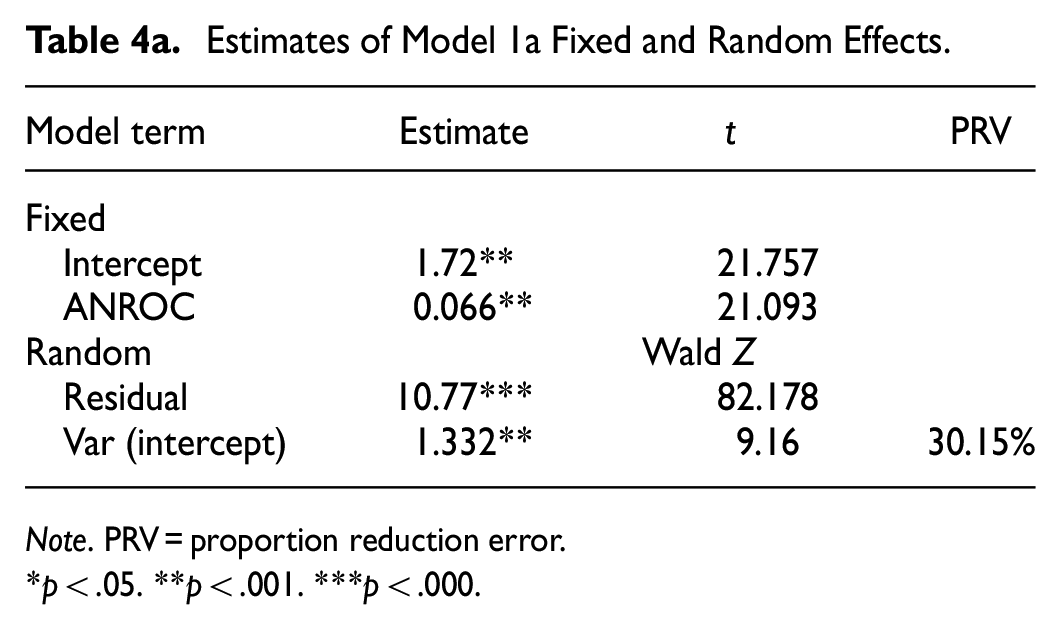
Note. PRV = proportion reduction error.
p < .05. **p < .001. ***p < .000.
Estimates Model 1b Fixed and Random Effects.

Note. PRV = proportion reduction error.
p < .05.**p < .001.***p < .000.
Level 2 Model
The level 2 analysis estimates the fixed and random predictors for all individual-level and aggregated group-level predictors (Table 5). Here, the intercept and slope are adjusted for each of the 278 neighborhoods—considering the variability and range of values of individual variables in block units nested within each neighborhood (group). The census block units within each neighborhood represent a cluster group. In other words, the estimated parameters—intercept and slope are considered random and expected to vary between the neighborhoods. Therefore, the values of the variables in the block units could vary within and between the level 2 neighborhoods. The intercepts of each neighborhood are the count of robbery incidents—that is, the block unit outcome adjusted for the predictor variables Xn. The slope β nj represents the effects of each predictor within each neighborhood group. Therefore, the neighborhood group level analysis estimates the between neighborhood group models using the within-group parameters—intercept and slopes. The probability of between-group variability of intercepts and slopes provides the platform for the second-level interrogation of the data set. The first research question for the second level analysis based on random and varying intercepts is: do the mean block unit count of robbery incidents vary across the neighborhoods? The answer to this question provides information on the level of robbery incident concentration or the effectiveness of crime control in each neighborhood concerning block unit values of the predictor variables. The second question based on the probability of randomness between group variability of the slopes is: do the effects (slopes) of the predictors on the block unit count of robbery incidents vary across the group-level neighborhoods? This finding will clarify the effect of the predictors on the neighborhood-level concentration of robbery incidents.
Estimates of Model 2 Fixed and Random Effects.

Note. PRV = proportion reduction error.
p < .05.**p < .001.***p < .000.
The multilevel model thus partitions the variation in the outcome variable between blocks and neighborhoods, examining the differences in outcome between the City’s 13,789 blocks and its 278 neighborhoods. Also, the examination of spatial lag, the commonality, and spatial influences between close-by areas, aids the accommodation of complex data structures where single-level regression may not provide a complete account of the standard errors. The estimated Moran’s “I” scores of the Queen Contiguity matrix (0.260) and the Rook contiguity matrix (0.2728) for the outcome variable were high and significant (p = .0001), suggesting that the spatial processes which stimulate the distribution of street robbery events within Baltimore city neighborhood blocks are not arbitrary.
Estimation of Interaction Effects
The estimation of interaction effect is a level 2 model with fixed level 1, level 2, cross-level interaction predictors, and randomly varying intercepts. The interaction effect of the sociodemographic risk factors on the ANROC (physical environment risk) measure is as follows:

This model estimates the fixed and random predictors for all the individual level predictors, the aggregated group level predictors, and the cross-level interaction effects (βnXij × Zij), Table 6. To further explain the variability within neighborhood models, neighborhood-level sociodemographic variables are introduced as cross-level interactors to moderate the effect of the ANROC variable on the concentration of robbery within the neighborhoods. Six cross-level interaction variables added to the level 2 model comprise the within-neighborhood ANROC and a neighborhood-level sociodemographic variable. The hierarchical structure of the multilevel model allows the estimation of the impact of each predictor for block-level data within each neighborhood. Thus aside from the fixed estimation of the predictor coefficients across all the enumerated blocks in the study area, it precisely estimates level-one regression parameters for each neighborhood group. This way, the group-level parameters—intercepts and slopes (predictor coefficients) can be randomly adjusted to determine their effects on the outcome. This process includes examining the covariance information between the intercepts, slopes, and residual variances associated with the two structural parameters. Thus just like the structural parameters, the block-level estimation errors are not assumed constant through the study area but may vary within the neighborhood groups (Heck & Thomas, 2009).
Estimates of Fixed and Random Effects for Model 3.

Note. PRV = proportion reduction error.
p < .05. **p < .001. ***p < .000.
Results
Risk Terrain Modeling
The risk terrain model is the linear operationalization of the spatial influence of risk factors on crime distribution as density or proximity. The results of the RTMDx analysis show that of the 20 risk predictors entered in the physical environment, 18, except for parks and pawn shops, recorded significant risk values related to the spatial distribution of street robbery in Baltimore City.
Table 1 lists each of the 18 significant risk factors, the type of spatial operationalization, the spatial influence of the risk factor, and the estimated relative risk value (RRV). With this result, the risk variable, drugs—representing illicit drug sales locations—recorded the highest relative risk value (RRV = 6.69). This result means proximity to places with a high density of illicit drug selling points increased the likelihood of street robbery by 6.69 compared to cells or places with risk value 1. The prostitution arrest points (RRV = 3.27), and offender anchor points (RRV = 3.113), followed the illicit drug risk factor. Comparatively, the RRVs indicate that places of illicit drug arrests present twice the risk of influencing street robbery than prostitution arrests and offender anchor points. However, the spatial influence of offender anchor points representing locations where offenders reside spread over 700 ft., five times the spatial influence of the illicit drug risk factor—spread only within half a block length (140 ft.).
Additionally, the location of public housing (2.06), gambling arrests (1.944), general merchant shops (1.78), bank ATM (1.56), and restaurants (1.55) recorded higher RRV’s in that decreasing order (Table 1) compared to barbing saloons which recorded a much lower risk (RRV = 1.52) to street robbery. However, the barbing saloon had a much broader spatial reach of 840 feet—a six times higher spatial estimate than the five preceding risk factors. The locations where bars and clubs are present also had a much lower RRV (1.47); its risk effect on street robbery, however, extended over two and a half block units (700 ft.). Similarly, grocery stores recorded a lower RRV (1.46); however, its risk influenced the street robbery spread over three blocks (840 ft.). Finally, though rail stations are the least risky of all the factors—being 4.7 less predictive of street robbery compared to illicit drug arrest points, it extends six times across more block space compared to the latter. Generally, there is much variability in the distribution of risk estimates and spatial influence between the predictors. Using ESRI ArcGIS raster calculation features, the values of the 18 significant risk predictors were subsequently aggregated across the 131,721 cells or places within 13,777 census blocks in Baltimore City to derive an average physical environmental risk estimate or ANROC for each census block. The ANROC (aggregated measure of relative risk) values ranged from 0 to 192.637 with a mean and standard deviation of 6.134 and 10.157, respectively. Table 2 summarizes the descriptive statistics of the outcome and predictor variables.
Multilevel Models
The assumption that the grand mean of the block-level count of street robbery incidents is 0 is invalid. In Table 3, the null model fixed effects of the intercept ϒ00 (grand mean) of the neighborhood-level distribution of street robbery incidents is 1.721. This value represents an average expected log count of robbery incidents per block within a neighborhood. In addition, the random effect estimate of the group level (neighborhood) intercept (σ2
Model 1
Following the null model, the fixed effect of the ANROC on the street robbery was estimated, Table 4a. The ANROC is the block-level aggregate risk value of environmental predictors of street robbery incidents earlier analyzed with the Risk Terrain Model (RTM), Table 1. The fixed effects estimates, Table 4a, show that ANROC had a significant relationship (β = .066, p = .001) with the block-level robbery count across the City. The addition of the ANROC predictor (model 1), however, adjusted the variation in the intercept (random effect estimate) down from β = 1.907 to 1.332 (Wald Z = 9.16, p = .000). The effect of ANROC was 0.066 for every one unit change per block level unit. At this stage, we did not estimate the random effect between neighborhoods of the environmental ANROC predictor but a reduction in variance as σ2BN − σ2BM1)/σ2BN. Where σ2BN is the neighborhood variation in mean robbery count for the null (no predictor) model, and σ2BM1 is the neighborhood intercept variance—model1. The difference between neighborhood variance (σ2BN) in the average block-level count of street robbery was 1.907 in the null model. With the addition of the ANROC (Table 4a), the proportional reduction between group variance is 30.15%. In other words, the block-level differences of ANROC within the neighborhoods account for about 30.15% of the variation in the average count of street robberies between the neighborhoods. However, examining the impact of related sociological variables on this prediction is equally essential. Since even with the introduction of ANROC, the Wald Z test is 9.16, suggesting that significant variability in street robbery counts between the City neighborhoods still requires explanation (See Heck et al., 2010). Subsequently, we estimate the six individual-level regression predictors anticipated for this study. Similar to the ANROC variable (Table 4a), the fixed effects Table 4b indicate that the variables—Percent Under 18, Percent Female-Headed Households, Percent Renter, Total Population, ANROC, and Racial Heterogeneity were significant (p < .001). However, while the rest of the variables had a positive coefficient, the Percent under 18 (−0.007) was negative, suggesting that the count of robbery incidents in the blocks decreased with the increasing population of residents under 18. The effect of the ANROC variable remained significant but decreased from 0.066 to 0.059 (Table 4b). The change in the ANROC coefficient suggests that the added variables affected the impact of the environmental risk factor on street robbery events across the blocks (See Heck et al., 2010). The second reduction in variance estimate calculated in model 1b (Table 4b) results in a 20.12% reduction in the variance of average block-level robbery count between the neighborhoods with the introduction of the additional block-level variables.
Model 2: Aggregated Level Effects
Alongside the environmental variable—ANROC, five block-level sociological variables and six neighborhood-level (aggregated) variables, including an aggregated ANROC predictor, are introduced to test their fixed effect on the block-level distribution of street robbery incidents, and compositional effects at the neighborhood level. This analysis also estimated the random effect block of the intercept and the random effect of the ANROC at the neighborhood level. Table 5 details the fixed effects estimates of the 11 variables. The level 1 fixed predictors, ANROC, Percent Under 18, Percent of Female-Headed Households, Percent Renter, Total Population, and Racial Heterogeneity, significantly predicted the count of robbery incidents at the block level across the City (p < .001). Interestingly, street robbery in the blocks decreased with an increase in the percentage of the under-18 population (β = −.0036, p = .001) and the percentage of female-headed households (β = −.0045, p < .001), respectively. The block-level ANROC effect on the count of robbery incidents decreased (β = .055) with the addition of the neighborhood-level ANROC predictor and the sociological variables. Individually, the impact of the neighborhood-level sociological predictors was less homogenous. It is evident that among the sociological variables, only the Percent Under 18 (β = −.033, p < .001) and Racial Heterogeneity (β = 2.2, p < .001) had a compositional effect at the neighborhood level. Also, at this group level, there was significant variation in the average count of robbery incidents (grand mean intercept: ϒ00) in the block-level units between the neighborhoods (β = 1.69, p = .000). The neighborhood level intercept changed from 1.064 to 0.76. The ANROC value varied significantly between the neighborhoods and covaried with the neighborhood-level average count of robbery incidents (intercept), Table 5. The third reduction in variance estimated between model 1 and model 2 results in a 28.57% reduction in the average block-level robbery count between the neighborhoods (Table 5) with the introduction of neighborhood-level variables in model 2.
Model 3: Relative Risk (ANROC) Interaction Effect
In the model 1 analysis, the ANROC variable was significantly related to the count of robbery incidents at the block level. However, by the model 2 analysis, the aggregate ANROC value equally varied significantly between the neighborhoods—having a random effect of β = .005, p < .001. In other words, the impact of crime attractors, generators, and contextual physical risk factors -representing the City’s environmental risk terrain modeled and aggregated as ANROC value varied across the neighborhoods. It is possible to categorize neighborhoods with characteristics that impact the block-level count of street robbery incidents for diverse ANROC values. Since the effect of the ANROC risk factor varies between the neighborhoods, we examine the relationships between neighborhood-level sociological variables and the individual-level ANROC variable.
The interaction effect of the neighborhood-level total population on individual level ANROC variable significantly impacted the concentration of robbery incidents (ϒ = −.0007, p<.05). This result suggests that the aggregate level total population moderates the effect of the within-group ANROC variable on street robbery concentration in the neighborhoods. However, the results showed that the neighborhood-level ANROC variable also moderates the within-neighborhood effect of the ANROC variable on street robbery concentration (ϒ = −.0038, p < .001). In addition, none of the other examined neighborhood-level variables had a moderating impact on the within-neighborhood effect of the ANROC variable (p > .05). The random effect variance component for the neighborhood clusters (Wald Z = 7.153, one-tailed p = .001) was further reduced by 27.76% with the estimation of cross-level interaction effects -and variation due to ANROC by 11.46%. The aggregate ANROC, under 18, and racial heterogeneity variables remained significant (Table 6).
Discussion and Conclusion
Tables 3 to 6 show the multilevel models’ parameter scores for fixed and random effects. The regression analysis results show that the expected average count (γ00) of street robbery incidents conditional on the absence of predictor variables is 1.907 for any random block in the City of Baltimore. The random variance of robbery incidents due to the effect of neighborhoods decreased by 30.15% for any random block by introducing risks due to the physical environment (ANROC) at the individual block level. The significance (p < .001) of the variation in the null model, level 1 outcomes, and level 2 intercepts indicates non-trivial clustering of street robbery incidents at the neighborhood level. At level 1, all six estimated individual predictors are significant. However, the Percent Under 18 variables had negative coefficients in models 1b and 2, and the Percent female-headed households in model 2, suggesting that street robbery incidents in the blocks across the City of Baltimore decrease with an increasing percentage of the two variables, considering the variables neighborhood effect. Thomas et al. (2020) have related such less impactful findings to the level of unreported crime data to police that is often rampant in socially disorganized neighborhoods. They note that the rate and intent to report offenses to the police vary across neighborhoods. They may be less in socially disorganized neighborhoods defined by high racial heterogeneity, structural disadvantages, mistrust, and legal cynicism. Therefore, the use and impact of the ANROC measure would be less useful in situations of low and attenuated crime reporting to the police, notable in socially disorganized neighborhoods.
The block-level ANROC impact is positive and significant (γ10 = .059, p < .001), predicting that blocks with high physical environment risks would have higher street robbery incidents within Baltimore neighborhoods. The introduction of the remaining level 1 predictor (Table 4b) decreased the impact of the ANROC predictor by 10.6%. The five variables significantly impacted the count of robbery events at this level. Adding the new predictors at level 1 reduced the neighborhood-level variation of street robbery by 20.12%, indicating that the added predictors explained some changes in the block-level concentration of street robbery-across neighborhoods.
Model 2 (Table 5) estimated 16 parameters in total. These include six individual-level and six aggregate neighborhood-level variables. Like Model 1, five individual-level variables entered in Model 2 significantly impacted the distribution of street robbery events. Except for the individual racial heterogeneity variable, which had no significant impact. While percent renters, a corollary for the percent homeownership, was positively related to the distribution of robbery incidents in models 1 and 2, other studies have reported a negative relationship (McNulty, 2001). Possible explanations for the different results would include the type and social and environmental area under research, the level of crime prevention measures, and the research plan and measurement constructs. The individual-level total population coefficient was significant and positive in models 1 to 3. This result contradicts RAT, according to which a higher population should provide better guardianship. However, at the aggregate neighborhood levels (models 2 and 3), notwithstanding, the total population coefficient conformed to RAT. This observation explicates the significance of examining the multilevel effects of the variables for precision-driven crime control policy development and strategic intervention purposes. Within Baltimore City’s social and environmental structure at the block level, offenders and victims may constitute a standard proportion of the population, manifesting street robbery at any population value. Urban areas increase household crimes, burglaries, and thefts by 32% and 16%, respectively. While living in inner-city neighborhoods increases these crimes by 80% and 48%, respectively, due to proximity to potential offenders (Tseloni, 2006). It is equally important to reiterate that the coefficients of the individual level Under 18 and the Percent Female-Headed Households were negative and significant—indicating that the count of street robbery events reduced across the blocks with increasing levels of the two variables. These variables theoretically have been related to the increasing crime rate (Borgess & Hipp, 2010; Shaw & McKay, 1942). The estimates of Under 18 and Female-Headed Households’ influence on Baltimore City street robbery in model 2 do not agree with the social disorganization theory explanation of neighborhood crime mentioned earlier in the paper. This result is another notable discrepancy from theory requiring an explanation. It is possible that the alternate areas with higher average income, though they reduce social disorder, tend to induce crime due to the concentration of more lucrative targets (Hipp, 2007). Therefore, areas of lower economic prospects identified with a higher proportion of female-headed households and a higher proportion of Under 18 residents could have lower street robbery estimates comparatively. The RAT explains that offenders would be attracted to areas with more lucrative targets. However, Tseloni’s (2006) examination of the impact of neighborhood watch programs on property crimes found that single-parent households significantly increased burglaries and thefts. In addition, the household characteristics covaried significantly between the area units. However, Tseloni (2006) did not control for the types and lucrativeness of the theft and burglary targets. In contrast, the interaction effect of the single-parent households enhanced the impact of neighborhood watch programs on property crimes.
Again, we are principally interested in estimating the variance components at this level. In model 2, the ANROC estimate is defined as randomly varying, changing the intercept and the predictors estimates from what we observed in model 1b, Table 4b. It is also important to note that the randomly varying ANROC slope is significant, suggesting that the risk of street robbery in the blocks due to the built environment varies between neighborhoods. Similarly, Jones and Pridemore (2019) showed that micro and macro-level variables affected street-level violent and property crime. Jones and Pridemore (2019) conducted their multilevel test using a negative binomial regression and also controlled for spatial dependence.
The results suggest that neighborhoods with higher average ANROC value (built-up environment risk) record more block robbery incidents. The group-level ANROC is positive and significant (γ01 = .07, p < .001). Similarly, the neighborhood level coefficient for Percentage Racial Heterogeneity is positive and significant (γ06 = 2.2, p < .001). This result suggests that increasing racial heterogeneity in a neighborhood increases the count of robbery events in the blocks. Heck et al. (2010) noted that parameter estimates would likely differ between single-level and multilevel models. Comparatively, parameter estimates of the street robbery count (.0597) of the individual level generalized linear model (GLM) for the fixed effects of the ANROC predictor, Table 4a, differed from the group level model estimate (.0552), Table 4b. As explained in Heck et al. (2010), the significant difference between the standard errors of the estimates, GLM (.00312), and multilevel GLM (.01619) affirms the expectation of group-level clustering in the data. The standard error of the group-level model is 80.7% larger than the individual-level GLM.
Model 3 (Table 6) estimated 21 parameters, including 7 individual-level, 6 neighborhood-level, and 6 cross-level interaction variables. The fixed effects section indicates that individual neighborhood predictors affect street robbery except for racial heterogeneity and the Under 18 predictors. The fixed effects parameters suggest that aggregate Percent under 18, Aggregate ANROC, and Aggregate Racial Heterogeneity affect street robbery distribution. Compared to individual-level racial heterogeneity in models 2 to 3, the aggregate effect supports the observation that racial heterogeneity may significantly impact crime in broader networks more than in local block-level networks (Hipp, 2007). In a related multilevel analysis, Velez (2001) found that individual victimizations at the level of micro household units reduced in macro unit urban neighborhoods that enforced public social controls. Valez’s findings imply that an increased level of public social control at the neighborhood level has a far-reaching effect on individual household safety.
Also notable is that the estimated slope variance for ANROC is significant (Wald Z = 4.92, p ≤ .001), suggesting that the level of risks of street robbery due to the built environment varies across neighborhoods. These findings partially support the study’s aim of identifying neighborhood-level explanations for the relationship between built environment variables and street robbery concentration. The six cross-level interaction variables introduced as moderating mechanisms to enhance or diminish the magnitude of the impact of ANROC on street robbery estimate the interaction effect as a measure of the degree to which the relationship between the predictors and street robbery depends on an intervening variable (Hamilton, 1992). For instance, the impact of the individual-level ANROC variable on the street robbery in model 3 is positive and significant (γ0x = .099, p < .001), and the interaction between the individual-level ANROC variable and the neighborhood level (group) ANROC variable is negative and significant (γ0x = −.0038, p < .001). The interaction effect measures the impact of the individual-level ANROC variable on street robbery when the magnitude of the individual ANROC* aggregate ANROC variable remains constant (see Hamilton, 1992). For instance, if the former was the only interaction effect of the individual ANROC variable, the estimated total impact of ANROC will be the sum of the magnitude of both coefficients (Hamilton, 1992; Heck & Thomas, 2009; Heck et al., 2010). Then, applying Hamilton’s directions to model 3, the full magnitude of the impact of the ANROC variable will be 0.095 when the average neighborhood-level ANROC coefficient is constant. The vital information derived here is that the aggregate ANROC variable’s function at the neighborhood level moderates the individual block-level functions of the same variable. Since this influence was significant (p < .001), the inference is that the built-up environment at the neighborhood level across the City of Baltimore varies in the magnitude of its impact on the distribution of street robbery. Tseloni (2006) found that interaction, household, and area effects co-jointly explained significant variation in property crime in Britain. Tseloni (2006) also applied a random effects multilevel model but had households as the microunits and British census-designated areas as the community-level macro units. Tseloni (2006) showed that the characteristics of the micro units (household), like the block level ANROC variable in this study, varied across the community macro units.
However, another significant cross-level effect evidenced in model 3 is the interaction between the individual-level ANROC variable and group-level average Total Population variable in the blocks. This relationship is estimated to be positive and significant (γ0X = .0007, p < .05). This interaction estimates the magnitude of the cross-level effect of the two predictors on street robbery when the aggregate Total Population variable is held constant. It is pertinent to clarify that though the neighborhood level aggregate Total Population is insignificant (γ0x = −.0005, p = .841), its interaction effect with ANROC is—moderating the latter by a magnitude of 0.0007. Therefore, the total effect of the Total Population is 0.0086. This result suggests that the moderating effect of aggregate Total Population positively impacts street robbery events in the blocks as the population at the neighborhood level increases. Suppose the total population exemplified in RATs could serve as a proxy for guardianship of crime targets when placed beside theoretical persuasions of social efficacy and reduced crime in neighborhoods. In that case, this result contradicts the possible intervening effects of increasing population in crime reduction at the neighborhood level in the City of Baltimore. Generally, among the six cross-level interaction parameters estimated by this model, Aggregate Percent under 18, Aggregate Percent Female Headed Household, Aggregate Percent Renters, and Aggregate Racial Heterogeneity do not moderate the within-neighborhood ANROC impact on street robbery distribution. Notwithstanding, the impact on the street robbery of the cross-level interaction between the individual ANROC variable and the neighborhood level ANROC variable on the one hand, and the neighborhood level Total Population variable on the other, were able to diminish the available variance of built environment risk across the neighborhood (Wald Z = 4.346, p < .001) from its previous level in model 2. Similarly, the available average intercept variation across the neighborhoods reduced (Wald Z = 7.153, p < .000) from model 2 levels and is significant. This result means that the function of the two estimated interaction parameters influences the variation of the concentration of street robbery events across the neighborhoods—signified by an additional 27.76% reduction in the variance component of street robbery counts across the neighborhoods and 11.66% variation in ANROC (Table 6). Specifically, the magnitude of a predictor’s coefficient does not depend solely on other predictors but on cross-level interactions between the predictors (Heck et al., 2010). However, the Wald Z score indicates that despite the added neighborhood and the interaction level variables, there remains significant unexplained variance in the intercepts and slopes.
In conclusion, the goal of this article was threefold. The first was to create a single environmental measure of risk based on spatial attractors and generators of street robbery. The second goal was to assess the impact of the environmental risk factor and other sociological predictors of crime on street robbery using a hierarchical generalized linear model. Moreover, finally, the third goal was to identify the moderating effect of the predictors on the environmental risk variable. Researchers continue to refine these analytical and conceptual processes to understand the forces that influence and regulate the distribution of crime across space. These forces operate at different dimensions of environmental and sociological communities and neighborhoods (Heck & Thomas, 2009). Models 1 to 3 explain significant variation in individual block-level distribution and neighborhood-level clustering of street robbery events in Baltimore City. Of particular mention are the environmental risk factor, ANROC, which significantly impacted street robbery at the level of block units and the aggregate neighborhood level. Aggregate level ANROC also moderated the capacity of block-level physical and social environments to influence street robbery. The ANROC accounts for the significant variation of street robbery across neighborhoods, concurrently examining all the risk factors and interaction effects. Hipp’s (2007) noted that the geographic area that defines the social interaction of residents and the geographic network important for crime control should determine the size of the geographic region for constructing variables for the structural enablers of crime. Crime reduction strategies require linkages with neighboring blocks. Greater neighborhood residential stability fosters cohesion and endears responsibility to the maintenance of civility and crime reduction (Adams, 1992; Bolan, 1997). However, this research has its limitations. The main research limitation is the omission of critical information about sociodemographic and physical environmental factors, which were not incorporated in the ANROC because they are not accessible, unavailable, or not correctly configured for statistical analysis. Second, while the estimated models explain the multilevel effects, it only estimates the interaction effect between ANROC and the other variables. A complete model precision would require estimating the effect of interactions between all pairs of variables—in which case, it underestimated the total impact of the variables on street robbery.
Notwithstanding these limitations, the results of this analysis provide some implications for intervention policies. The resulting outcomes demonstrate that not all assumptions about the effects of ANROC and the other sociodemographic variable remain true at different levels of the analysis. Regarding the modeling to determine statistical impact, this study has shown the relevance of multilevel models in spatial analysis to avert the imputation of fallacies and biases that may result from treating group-level spatial effects on crime distribution as individual unit effects. The results show that distinct localized and broader effects on community sociodemographic forces impact crime distribution (Hipp’s, 2007). Therefore, the general implication of the findings of this research is its potential for understanding multiple spatial-level interactions of factors that influence street robbery distribution in Baltimore City for crime prevention purposes. The specific implications are as follows: places with a higher concentration of physical environmental factors -a high ANROC risk—require a requisite level of security monitoring and law enforcement intervention. Second, it looks at the relationship among some critical sociodemographic forces at the micro and macro level unit of street robbery distribution in the city.
Finally, of particular significance is the gap in unexplained variances of the outcome variable—suggesting the requirement of additional research to enlist a more comprehensive compilation of operating risk factors—both environmental and sociodemographic, within Baltimore City. The results support the significance of identifying data on the risks and protective factors of violent crimes such as street robbery. Future studies could examine factors that make some neighborhoods more resilient to street robbery activities than others by interrogating multiple levels of neighborhood influence and interactions within and beyond the scope of the present report.
Footnotes
Declaration of Conflicting Interests
The author declared no potential conflicts of interest with respect to the research, authorship, and/or publication of this article.
Funding
The author received no financial support for the research, authorship, and/or publication of this article.
Data Availability Statement
The datasets generated during and/or analyzed during the current study are available from the corresponding author on reasonable request.