
Abstract
Growth mixture model (GMM) is a flexible statistical technique for analyzing longitudinal data when there are unknown heterogeneous subpopulations with different growth trajectories. When individuals are nested within clusters, multilevel growth mixture model (MGMM) should be used to account for the clustering effect. A review of recent literature shows that a higher level of nesting was described in 43% of articles using GMM, none of which used MGMM to account for the clustered data. We conjecture that researchers sometimes ignore the higher level to reduce analytical complexity, but in other situations, ignoring the nesting is unavoidable. This Monte Carlo study investigated whether the correct number of classes can still be retrieved when a higher level of nesting in MGMM is ignored. We investigated six commonly used model selection indices: Akaike information criterion (AIC), consistent AIC (CAIC), Bayesian information criterion (BIC), sample size–adjusted BIC (SABIC), Vuong–Lo–Mendell–Rubin likelihood ratio test (VLMR), and adjusted Lo–Mendell–Rubin likelihood ratio test (ALMR). Results showed that accuracy of class enumeration decreased for all six indices when the higher level is ignored. BIC, CAIC, and SABIC were the most effective model selection indices under the misspecified model. BIC and CAIC were preferable when sample size was large and/or intraclass correlation (ICC) was small, whereas SABIC performed better when sample size was small and/or ICC was large. In addition, SABIC and VLMR/ALMR tended to overextract the number of classes when there are more than two subpopulations and the sample size is large.
Introduction
Multilevel growth mixture model (MGMM) is a relatively new modeling technique for extracting unknown subpopulations in multilevel longitudinal data. This technique integrates multilevel modeling, finite mixture modeling, and structural equation modeling (Asparouhov & Muthén, 2008; B. Muthén, 2004). The multilevel aspect of MGMM is attractive to applied researchers because longitudinal data are often collected through cluster sampling, which creates multilevel data structure with repeated measures nested within individuals and individuals further nested within organizations. Some examples are students nested within classrooms/schools/neighborhoods (e.g., Dettmers, Trautwein, Lüdtke, Kunter, & Baumert, 2010), children/couples nested within families (e.g., Jenkins, Dunn, O’Connor, Rasbash, & Behnke, 2005; Pruchno, Wilson-Genderson, & Cartwright, 2009), individuals nested within countries (e.g., Matsumoto, Nezlek, & Koopmann, 2007), clients nested within therapists (e.g., Marcus, Kashy, & Baldwin, 2009), and individuals nested within organizations (e.g., Vancouver, 1997).With multilevel longitudinal data, unknown subpopulations can be extracted at the individual level as well as the organization level (Palardy & Vermunt, 2010). In addition, researchers can study the associations between organizational characteristics and individual growth patterns (note: in this article, the terms class and subpopulation are used interchangeably). It should be noted that other methods, such as item response theory (e.g., Bartolucci, Pennoni, & Vittadini, 2011), can be used to account for longitudinal data structure in the analysis of latent traits as well, but the focus of the current article is on MGMM. Due to space constraints, interested readers may find more detailed technical information on MGMM in Chen, Kwok, Luo, and Willson (2010). Also note that the current article uses many acronyms throughout; therefore, for reference, a list of these acronyms and what they denote is provided in the appendix.
To investigate the prevalence of the higher level nesting in growth mixture model (GMM), we reviewed 158 substantive articles with 196 GMMs found in the PsycInfo database between 2011 and 2013. Of these, authors described nesting structure in 85 GMMs (43%), none of which used MGMM to address it. Nevertheless, nine articles addressed the clustering by reporting a low degree of clustering or using adjusted standard errors.
Our review shows that multilevel longitudinal data are common, but when applying GMMs, many empirical researchers ignore the highest level of nesting, potentially violating the assumption of independence (e.g., Boscardin, Muthén, Francis, & Baker, 2008; D’Angiulli, Siegel, & Maggi, 2004). Some reasons for ignoring a level of nesting are avoidable, such as reducing analytic complexity and reducing the difficulty in achieving convergence in model estimation, while others are inevitable such as lack of identifiers (IDs) for higher level units.
The literature has demonstrated that if the nonindependence is not accounted for, parameter estimates and standard errors in a multilevel regression model could be biased (Moerbeek, 2004). In MGMM, ignoring a higher level of nesting structure could result in lower classification accuracy, overestimated lower level variance components, and biased standard errors, which affect significance tests for fixed effects (Chen et al., 2010).
In mixture modeling, one important yet challenging issue is extraction of the correct number of latent classes (e.g., Bartolucci & Murphy, 2015; McLachlan & Peel, 2000). In recent years, many researchers have investigated the performance of various model selection indices in identifying the correct number of classes in different types of mixture models with different data structures (i.e., Allua, 2007; Clark & Muthén, 2007; Henson, Reise, & Kim, 2007; Nylund, Asparouhov, & Muthén, 2007; Peugh & Fan, 2012; Tofighi & Enders, 2008; Yang, 2006). Although the types of mixture models used in simulation studies vary and the best performing indices differ, Bayesian information criterion (BIC; Schwartz, 1978), sample size–adjusted BIC (SABIC; Sclove, 1987), and the Vuong–Lo–Mendell–Rubin likelihood ratio test (VLMR; Lo, Mendell, & Rubin, 2001) consistently performed well for model selection with single-level data.
However, the influence of ignoring a level of nesting on class enumeration for MGMM has not yet been fully investigated. Because ignoring a higher level may be inevitable in some circumstances as described above, an understanding of fit index performance in those situations is warranted. As shown in previous studies on multilevel analysis (e.g., Chen et al., 2010; Meyers & Beretvas, 2006; Moerbeek, 2004), ignoring the highest level data structure results in the redistribution of variance from the ignored level (i.e., the organization/school level) to the adjacent level (i.e., the individual/student level). It is unclear if this redistribution of variance will affect model selection index performance. It is important to determine whether the recommended model selection indices can extract the correct number of classes when ignoring a higher level of nesting structure is inevitable and to provide researchers with recommendations on using these indices.
Purpose of the Study
The purpose of this study is to (a) investigate whether the correct number of classes can be identified using various commonly used model selection indices when the MGMM is misspecified to omit the higher level and (b) identify factors that affect the index performance for class enumeration when the model is misspecified. The current study extends work by Chen et al. (2010) in several ways. First, whereas Chen et al. focused on the accuracy of classification of individuals and the statistical properties of the parameter estimates (i.e., Type I error rate and statistical power) for each subpopulation, conditional upon the correct number of classes being identified, the current study addresses whether the correct number of classes can be enumerated using various model selection indices under both true and misspecified models. This is an important advancement for applying the MGMM given that individual class solutions and corresponding class models can only be further examined and interpreted after the correct number of classes is identified. To that end, the current study examines the efficacy of six commonly used indices for class enumeration in GMM.
Compared with Chen et al. (2010), the current study has been expanded to examine one additional design factor by including a true model with three latent classes. Furthermore, we apply some suggested cutoff values for comparing different information criteria between competing models (e.g., delta-BIC, Raftery, 1996) whereas previous studies examining the sensitivity of the information criteria did not account for the magnitude of that difference.
We begin by reviewing the development and specification of MGMM, followed by a brief review of various commonly used model selection indices, and a review of recent studies examining the model index performance. In the simulation study, we first examined a two-subpopulation case (Study 1), followed by a three-subpopulation case (Study 2), because the number of subpopulations may affect the model selection indices’ performance. In addition to the number of subpopulations, we investigated the effect of another type of model complexity in Study 3.
Brief Review of MGMMs
The development of MGMMs drew upon several lines of research (Palardy & Vermunt, 2010), namely, latent growth curve modeling (LGCM; Bollen & Curran, 2006), latent class growth analysis (LCGA; Nagin, 1999), and GMM (B. Muthén, 2004). Combining LGCM and LCGA, GMM is a more general modeling framework capable of examining both the unknown heterogeneous subpopulations and the random variation of the latent growth factors within classes. However, GMM does not consider the situation of multilevel data in which individuals are nested within organizations. Hence, GMM cannot handle nonindependence of individuals due to clustering. Existing research has explored methods of accounting for nonindependence of observations in mixture modeling and GMM (Asparouhov, & Muthén, 2008; Ng & McLachlan, 2014; Ng, McLachlan, Wang, Jones, & Ng, 2006). An extension to GMM, MGMM considers nonindependence of individuals by specifying a model for each level of the multilevel data. The model for the individual and organizational levels can be different, depending on whether heterogeneity is assumed and/or random effects at both the individual level and the organizational level growth trajectories are modeled. This article focuses on the more common MGMM with classification at the individual level (e.g., students being classified into different subgroups within schools; patients being classified into different subtypes within clinics) and no classification at the organizational level.
Brief Review of Model Selection Indices
A combination of substantive knowledge and statistical criteria has been recommended for selecting the optimal number of classes in GMM (B. Muthén, 2003). Generally, model selection statistics can be grouped into four categories: (a) information-based criteria, (b) nested model likelihood ratio tests (LRTs), (c) goodness-of-fit measures, and (d) classification-based statistics (Henson et al., 2007; Tofighi & Enders, 2008; Vermunt & Magidson, 2002). Among these categories, the information-based criteria and the nested model LRTs are the most recommended for determining the number of classes (Henson et al., 2007; Nylund et al., 2007; Tofighi & Enders, 2008). Hence, the model selection indices from these two categories are the focus of this study and are briefly reviewed below.
Information criterion (IC) indices are based on the log-likelihood value of a fitted model and typically penalize model complexity and/or take sample size into account. IC usually takes the form of


where p is the number of free parameters in the model and N is the number of subjects. Generally, as a model becomes more complex (i.e., more parameters and larger p), the likelihood increases and
The IC statistics take both model fit and complexity into consideration. Lower values indicate better trade-off between model fit and complexity. Sometimes, the IC difference between two models is so small that the evidence to support one model over the other becomes very weak. Some guidelines for interpreting the absolute IC difference between two models have been proposed. Petras and Masyn (2010) recommended the “elbow criterion” to determine the optimal number of classes when using IC indices (i.e., AIC, BIC, SABIC). Specifically, they recommended graphing the values of IC indices against the increasing number of classes, and looked for the pronounced angle in the plot where the decrease of IC value dropped. As plotting for all replications was unrealistic, we used cutoff criteria that mimic looking for the “elbow point.”
Besides their statistical differences, the AIC and BIC also have different philosophical contexts (Bauer & Curran, 2003; Burnham & Anderson, 2004; Kuha, 2004; Weakliem, 2004). AIC aims at finding the model that minimizes the Kullback–Leibler (K-L) criterion, selecting an approximate model, and providing better predictions of the population parameters. On the contrary, BIC targets the “true” underlying model with the highest posterior probability. It depends on the purpose of model selection and the nature of reality when deciding which model selection index to use. AIC and BIC were designed for different applications, and both applications can arise in multilevel (growth) mixture modeling.
The nested model LRTs include the VLMR, the adjusted Lo–Mendell–Rubin likelihood ratio test (ALMR; Lo et al., 2001), and the bootstrap likelihood ratio test (BLRT; McLachlan & Peel, 2000). All these statistics are developed using LRT and test the null hypothesis that the restricted model with k − 1 classes fits the data as well as the less restricted model with k classes. The test statistic for a likelihood ratio (LR) test is defined by

where L0 and Lu are the maximized likelihood for the more and less restricted models, respectively (Agresti, 1996). Under the context of mixture model, the LR for (k − 1)-class model versus k-class model is not asymptotically distributed as a chi-square, so the normal chi-square difference test is not applicable. Therefore, Lo et al. (2001) derived an approximate reference distribution for the LR in the mixture context by extending Vuong’s (1989) work called the Vuong–Lo–Mendell–Rubin likelihood ratio test (VLMR). Furthermore, Lo et al. (2001) proposed an ad hoc adjustment to VLMR (i.e., ALMR—adjusted Lo–Mendell–Rubin likelihood ratio test), which is defined by
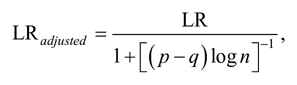
where
Review of Studies on Performance of Model Selection Indices
Recently, researchers have studied the performance of these model selection indices in nonclustered data in the context of latent class analysis (LCA; Nylund et al., 2007; Yang, 2006), GMM (Nylund et al., 2007; Peugh & Fan, 2012; Tofighi & Enders, 2008), latent profile analysis (Morgan, Hodge, & Baggett, 2016), latent variable mixture model (Henson et al., 2007), factor mixture model (FMM; Nylund et al., 2007), and latent Markov model (Bacci, Pandolfi, & Pennoni, 2014). A few studies have searched for the optimal model selection indices for clustered/multilevel data in LCA (Clark & Muthén, 2007; Lukociene & Vermunt, 2010) and FMM (Allua, 2007). Table 1 summarizes these studies, showing the models and indices examined, as well as the best performing or recommended fit indices for class enumeration in each study. As shown in the table, although the types of mixture models vary, they seem to agree on the use of SABIC, BIC, and VLMR/ALMR for model selection in single-level data.
Summary of Recent Studies Examining Performance of Model Selection Fit Indices in Mixture Models.

Note. Alphabetized fit indices. AIC = Akaike information criterion; AICc = corrected Akaike’s information criterion; AIC3 = A variant of AIC that uses 3p as the penalty term; ALMR = adjusted Lo–Mendell–Rubin likelihood ratio test; BIC = Bayesian information criterion; BLRT = bootstrap likelihood ratio test; CAIC = consistent AIC; CLC = classification likelihood information criterion; DBIC = Draper BIC; DIC = deviance information criterion; HQ-IC = Hannan–Quinn information criterion; HT-AIC = Hurvich–Tsai AIC; ICL-BIC = integrated classification likelihood (BIC approximation); ICOMP = Bozdogan’s information complexity criterion; LMR = Lo–Mendell–Rubin likelihood ratio test; MKT = multivariate kurtosis test; MST = multivariate skewness test; NBIC = sample size–adjusted BIC; NC-AIC = sample size–adjusted CAIC (aka SACAIC); NCS = traditional chi-square difference test; ND-BIC = sample size–adjusted DBIC; NEC = normalized entropy criterion; NHQ = sample size–adjusted Hannan–Quinn information criterion; NHT-AIC = sample size–adjusted HT-AIC; NICL-BIC = sample size–adjusted ICL-BIC; SABIC = sample size–adjusted BIC (aka NBIC); SACAIC = sample size–adjusted CAIC (aka NC-AIC); VLMR = Vuong–Lo–Mendell–Rubin likelihood ratio test.
A few studies have searched for the optimal model selection indices for clustered/multilevel data. In LCA, using standard error corrections for clustered data, Clark and Muthén (2007) found that for simple structure data (i.e., latent classes with parallel profiles), none of the studied indices performed well, whereas for complex data structure (i.e., latent classes with crossing profiles), BIC and SABIC performed relatively better. For multilevel FMM, which is a multilevel extension of the factor analysis model for cross-sectional datasets with a hierarchical structure, Allua (2007) found that BIC, SABIC, and ALMR performed better in situations when there was only one class in the population; AIC and ALMR performed better in situations when there were two classes. However, Allua (2007) did not identify any consistently well-performing model selection index for the multilevel FMM. Lukociene and Vermunt (2010) compared the performance of alternate fit indices in multilevel mixture model with focus on determining the true number of mixture components at the organization level. They raised the interesting point that the N for BIC and CAIC computations is unambiguous for single-level mixture evaluation but ambiguous for multilevel mixture evaluation. Their results supported defining N as the number of groups when picking classes that exist at the highest level.
In summary, the literature suggests BIC and SABIC performed best for class enumeration for both single-level and multilevel mixture models. However, no study explicitly examined which indices perform best when the higher level of nesting is ignored in the context of MGMM. In addition, none of the current widely used fit indices for class enumeration was designed/developed for testing multilevel models. It would be interesting to see if using the individual level N would be sufficient for the more common MGMM. To address this shortcoming in the literature, this study tests the performance of six commonly used model selection indices in MGMM with continuous outcomes, including AIC, CAIC, BIC, SABIC, VLMR, and ALMR, all of which except for CAIC are available in Mplus (L. K. Muthén & Muthén, 1998-2010). The performances of these indices are compared under the correct model specification, which includes the higher level of the nesting to accommodate the clustered data structure, and under the misspecified model, where the higher level is ignored. This study’s results can provide insights into the robustness of the model selection indices when a higher level in MGMM is ignored under a variety of design conditions as well as the best practice to use when such misspecification is inevitable.
Study 1: Two-Class Case
Method
Data generation
Data with two known subpopulations under a three-level model (e.g., repeated measures nested within students and students nested within schools) were first generated. The three-level model for data generation is shown below:
Level 1:

with

Level 2:


with

Level 3:


with

where the time variable
In this three-level model, four fixed effect coefficients (i.e., γ00, γ01, γ10, and γ11) and five variances and covariances of the random effects (i.e., σ2, τπ00, τπ01, τπ11, τβ00) needed to be specified. The average growth models for the two subpopulations were specified as follows so that Subpopulation A represents a low-start and slow-growing group and Subpopulation B represents a high-start and fast-growing group:
Subpopulation A:

Subpopulation B:

Based on the settings presented in Equations 2a and 2b,
Design factors
Previous simulation studies have identified some important design factors that may affect the performance of the model selection indices. First, the degree of class separation dramatically impacts enumeration of the correct number of classes; if the generated classes are well-separated, the correct number of classes is more easily identified (Henson et al., 2007; Tofighi & Enders, 2008). Second, the latent class mixing proportions have a substantial impact on class enumeration (Enders & Tofighi, 2008; Henson et al., 2007; Tofighi & Enders, 2008). In unbalanced situations where one latent class has an extremely low mixing proportion (e.g., 7% in Tofighi & Enders, 2008, 10% in Henson et al., 2007), the model is less likely to converge and the class enumeration is less accurate. Third, sample size influences model selection index performance in class enumeration, performing better with larger sample sizes (Henson et al., 2007; Tofighi & Enders, 2008). Given these findings, we manipulated five design factors: degree of separation, conditional intraclass correlation (ICC), number of clusters, cluster size, and latent class mixing proportions.
Degree of separation
We manipulated the magnitude of the

Mean growth trajectories with error bars for small

Mean growth trajectories with error bars for medium
Conditional ICC
We selected two levels of conditional ICC, .10 and .20, to represent small clustering effect and medium clustering effect (Hox, 2010). Based on the conditional ICC and
Number of clusters
We considered three levels for the number of clusters: 30, 50, and 80. Recently, Graves and Frohwerk (2009) systematically reviewed 27 studies using multilevel modeling from five journals devoted to school psychology research and practice. For the 27 studies, the cluster number (e.g., number of schools) had a mean of 28 and a minimum of 17. However, we use 30 as the minimal number of clusters because the multilevel modeling research design literature suggests at least 30 clusters are needed to provide unbiased estimates of fixed and random effects that can be expected to replicate in repeated samples from the same population (Hox, 2010; Kreft & De Leeuw, 1998). We included 50 and 80 as medium and high cluster number levels, which enables our simulation study to mimic applied studies with higher cluster numbers and/or in areas other than school psychology, and allows us to examine the impact of a broader range of cluster numbers and overall sample size combinations on the estimation of the MGMMs.
Cluster size
We selected two levels for cluster size: 20 and 40 individuals per cluster. Based on Graves and Frohwerk’s (2009) review, the average cluster size was 44 (SD = 43). The level of 40 individuals per cluster was close to the mean cluster size while the level of 20 individuals per cluster was close to the 50th percentile (n = 24).
To further justify the sample size conditions, we conducted a literature search in PSYCINFO (from year 2000 to 2011) for empirical studies applying GMM in different substantive areas. We found a total of 171 studies; however, only one recent study used MGMM (i.e., Tobler & Komro, 2010). After removing eight studies with extreme sample sizes, the overall sample size of the remaining 163 studies ranged from 115 to 5,914, with a mean of 969 (SD = 1,204). Based on the design factor levels of cluster number (30, 50, and 80) and cluster size (20, 40), the combined/overall sample size in our simulation study covered a wide range (i.e., from 600 to 3,200) that is common in applied studies in social sciences.
Mixing proportion
The mixing proportions of the two subpopulations were set to be balanced or unbalanced. In the balanced situation, mixing proportion was set to 50% and 50% for the two subpopulations. In the unbalanced situation, the mixing proportion was set to 25% for the low-start and slow-growing group and 75% for the high-start and fast-growing group, to mimic a situation in school setting where the majority of students develop their reading skills quickly (Nylund et al., 2007). We did not consider a more extreme unbalanced situation because previous research found that models with extreme population mixture proportions (i.e., 10% or less) of a subpopulation were less likely to converge and the class enumeration was less accurate (Henson et al., 2007; Tofighi & Enders, 2008).
In summary, the simulation used a 2 (degree of separation: low or medium) × 2 (cluster size: 20 or 40 cases) × 3 (number of clusters: 30, 50, or 80 clusters) × 2 (mixing proportions: 50%:50% or 75%:25%) × 2 (ICC: .10 or .20) factorial design to generate the data. A total of 500 replications were generated for each condition using the SAS 9.2 Proc IML procedure, yielding a total of 24,000 datasets (500 datasets × 48 conditions). For each replication, six different models—that is, 2 model specifications (true/misspecified) × 3 different class solutions with different numbers of classes (1, 2, and 3) = 6 models—were fitted using the Mplus 6.1 Mixture routine (L. K. Muthén & Muthén, 1998-2010); analyses were conducted using the MLR (MLR is a robust maximum likelihood estimator that uses a Huber-White sandwich approach to adjust standard errors for non-normality) estimator. The number of initial stage random start values was initially set to 50 and the number of final stage optimizations was set to 10. If there were any convergence issues during analysis, the number of random starts was increased.
Analysis
All 24,000 datasets had converged results for fitted models and a reasonable number of observations in each latent class (i.e., class size no less than 6% of the total sample size). The performance of a model selection index was measured by the proportion of replications in which the index retrieved the correct number of classes.
Criterion for determining success in class enumeration
For AIC, differences less than 2 suggest no credible evidence as to which model is better, differences between 2 and 4 weak evidence, differences between 4 and 7 definite evidence, differences between 7 and 10 strong evidence, and differences larger than 10 very strong evidence (Burnham & Anderson, 2002). We adopted the cutoff value of 4 points; specifically, for AIC to select the correct two-class solution, it had to satisfy two requirements. First, the two-class AIC had to be smaller than the one-class and three-class AIC. Second, the two-class AIC had to be 4 or more points smaller than the one-class AIC. Based on the K-L information theory, AIC differences can be converted to Akaike weight
Example of Relationship Between AIC Difference and Akaike Weight.

Note. AIC = Akaike information criterion; AW = Akaike weight; subscripts 1, 2, and 3 refer to one-class, two-class, three-class models, respectively; Δ3 = AIC3 − AIC2.
For BIC, differences less than 2 suggest weak evidence, differences between 2 and 6 positive evidence, differences between 6 and 10 strong evidence, and differences larger than 10 very strong evidence (Raftery, 1996). The difference in BIC can also be converted into relative probability. For instance, if the two-class BIC is 2 points less than the one-class BIC, the Bayes factor for a two-class model against a one-class model is 3 (i.e.,
For CAIC and SABIC, no guideline has been proposed before. We used 2 as their cutoff values because they are similar to BIC in computation.
As previously mentioned, different rules were used to select best-fitting models for VLMR and ALMR. Because these two indices use a significance test, when testing the k-class model (k > 1), there are two possible decisions. When the p value of these indices is equal or smaller than .05, the k-class model would be selected over the (k − 1)-class model; when the p value is larger than .05, there is a lack of evidence for significant improvement and therefore the more parsimonious model—that is, (k − 1)-class model—is selected (Lo et al., 2001). The procedure for determining the best model (see Figure 3) begins with the two-class model, and continues until a comparison of the k-class model, and the (k + 1)-class identify the k-class solution as the better model. We stopped at the three-class model because our interest was in whether the correct number of classes was identified and any decision other than the two-class solution would be considered a wrong decision.

VLMR/ALMR decision flowchart.
Difference between true and misspecified models
We examined how differently the indices performed under the true model (i.e., consider the higher level) and the misspecified model (i.e., ignoring the higher level). The accuracy of each index under the true and misspecified models was compared and differences were computed.
Impact of the design factors
ANOVAs were conducted to determine the impact of the five design factors on the fit indices’ class enumeration accuracy. The percentage of correct model identification was the analysis outcome (e.g., the outcome value is 90% if two-class model was selected for 450 out of 500 replications). Eta-squared (i.e.,
Results
Overall fit index performance
Figure 4 shows the average percentages of one-class, two-class, and three-class (or more) models identified by AIC, CAIC, BIC, SABIC, VLMR, and ALMR for all 24,000 datasets under both true and misspecified models. As shown in the figure, all model selection indices correctly identified the two-class solution (i.e., the correct solution) in most replications regardless of model specification (i.e., correctly specified or misspecified model). For the true model, BIC had the highest percentage of correct classification (98%), followed by SABIC and CAIC (97%), ALMR (90%), VLMR (89%), and AIC (76%). For the misspecified model, SABIC had the highest percentage of correct classification (91%), followed by BIC (82%), ALMR (81%), VLMR (80%), CAIC (78%), and AIC (66%). The difference in classification accuracy between true and misspecified models was 6%, 9%, 9%, 9%, 16%, and 20% for SABIC, VLMR, ALMR, AIC, BIC, and CAIC, respectively.
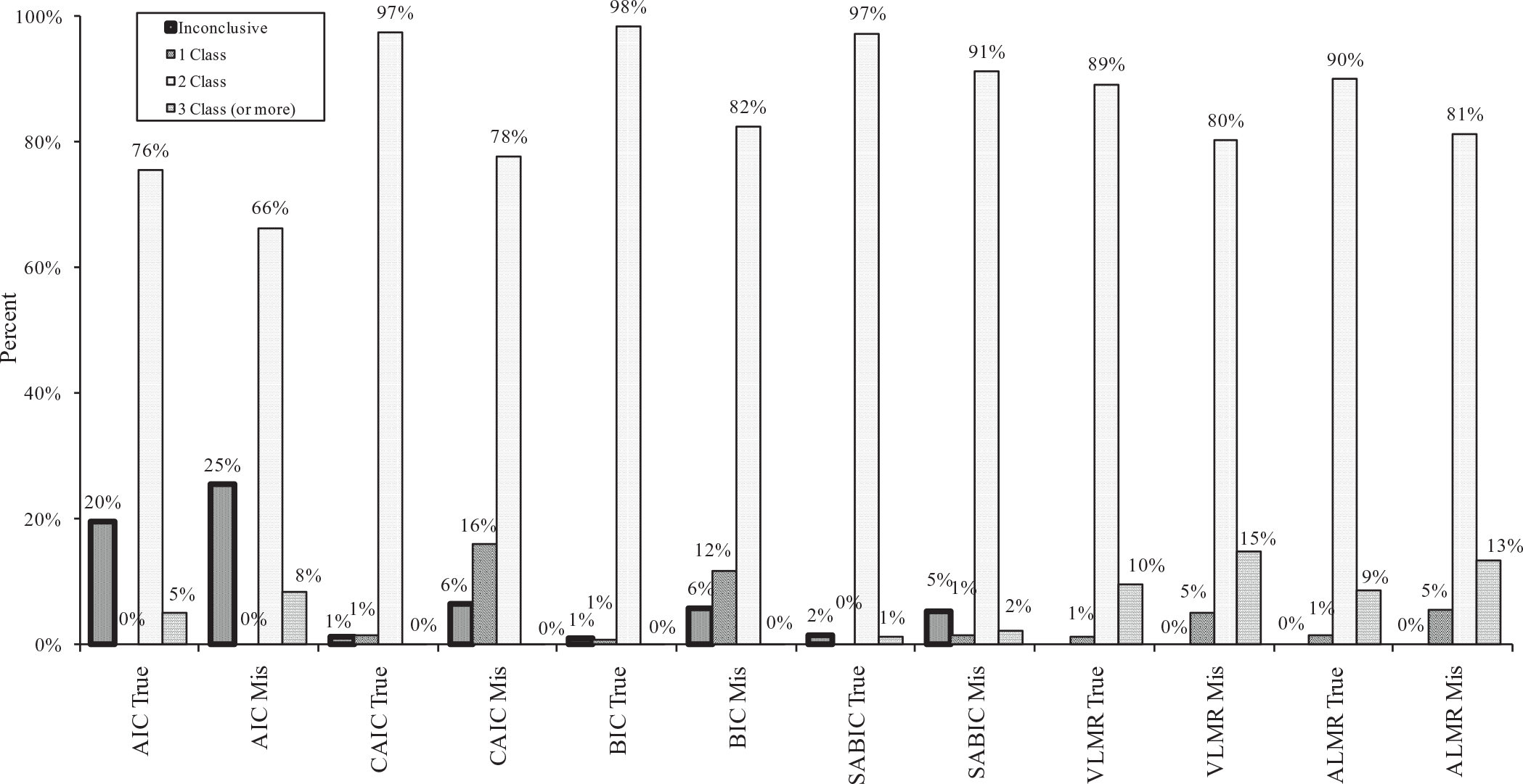
Percentage of one-, two-, three-class (or more) models and inconclusive classification identified by AIC, CAIC, BIC, SABIC, VLMR, and ALMR under true and misspecified models.
Under the true model, the proportion of inconclusive classification ranged from approximately 20% for AIC, to almost 0 for CAIC, BIC, and SABIC. More inconclusive classification appeared under the misspecified model, with AIC again having the highest proportion, followed by BIC and CAIC, and then SABIC. CAIC and BIC had a tendency to underextract the number of classes under the misspecified models, whereas AIC, VLMR, and ALMR tended to overextract the number of classes under both the true and misspecified models.
Effect of design factors
ANOVA results indicated that ICC, cluster number, and cluster size were the three most important factors. Table 3 shows the performance of the six model selection indices under both the true and false models as well as the difference between the true and misspecified models collapsed over the three factors.
Study 1, Study 2, and Study 3 Results Collapsed Over ICC, Cluster Number, and Cluster Size.
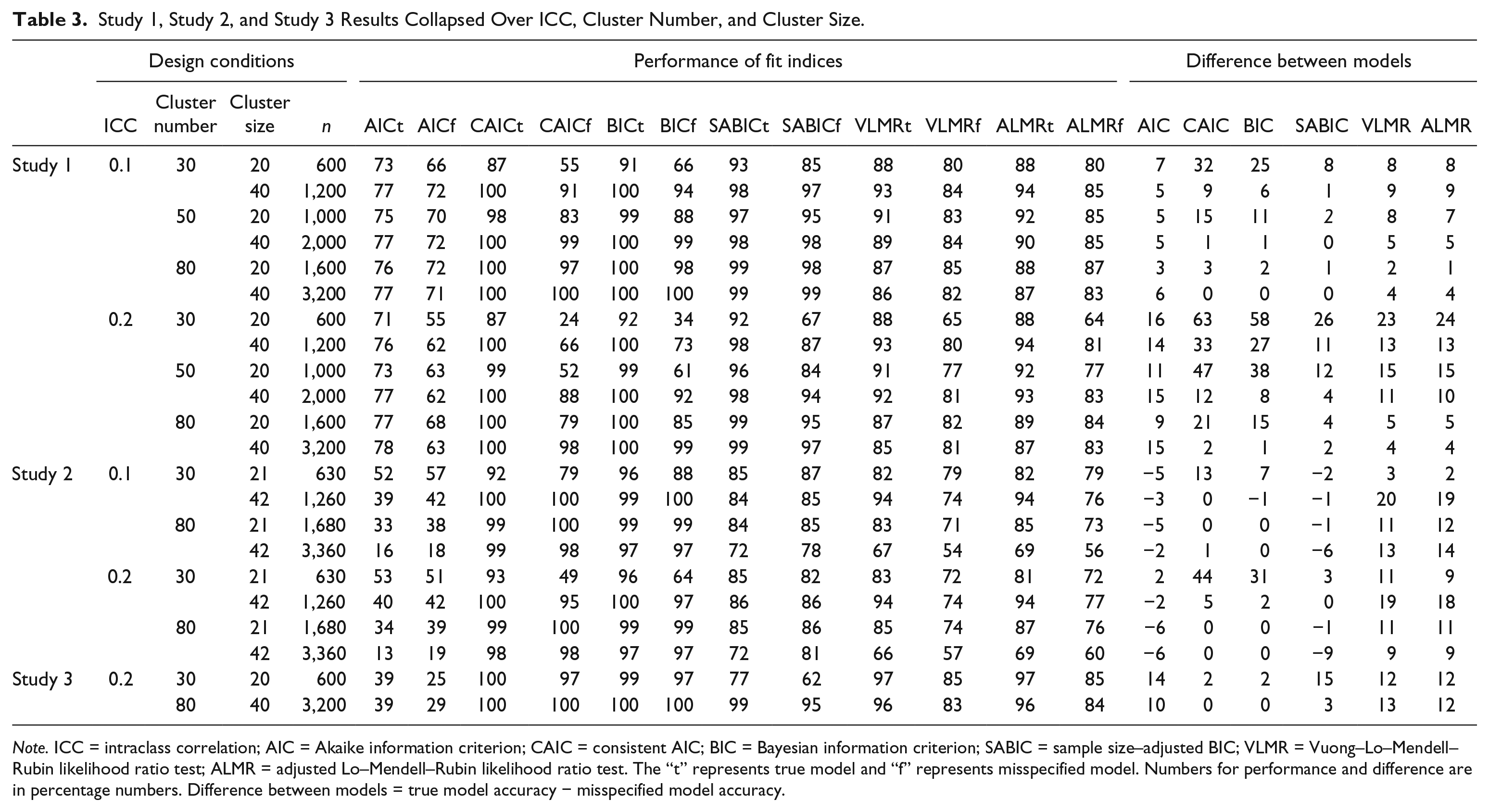
Note. ICC = intraclass correlation; AIC = Akaike information criterion; CAIC = consistent AIC; BIC = Bayesian information criterion; SABIC = sample size–adjusted BIC; VLMR = Vuong–Lo–Mendell–Rubin likelihood ratio test; ALMR = adjusted Lo–Mendell–Rubin likelihood ratio test. The “t” represents true model and “f” represents misspecified model. Numbers for performance and difference are in percentage numbers. Difference between models = true model accuracy − misspecified model accuracy.
ICC had a negative impact on all six model selection indices under the false model. The average accuracy of class enumeration decreased as ICC increased from .1 to .2 (
In general, cluster number and cluster size had positive effects on the accuracy of the IC indices. As cluster number and cluster size increased, the accuracy of class enumeration increased (
In addition, increasing
Study 2: Three-Class Case
Method
In Study 2, we examined the performance of the previously mentioned model selection indices in a three-subpopulation MGMM. According to Tofighi and Enders’s (2008) review, three-class models are also common in published studies using GMM. In addition, increased number of subpopulations might increase the difficulty of separating latent classes. Therefore, Study 2 can help determine whether fit index performance remains consistent in more complicated situations. The design conditions and analysis procedure remained mostly similar as those in Study 1 with a few modifications, which are described in the following sections.
Data generation
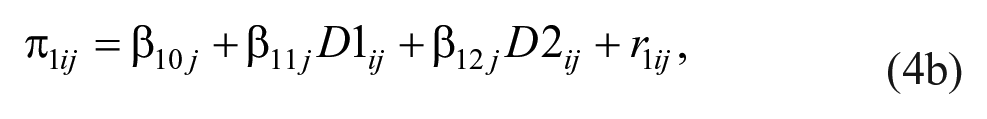
In Study 2, data with three known subpopulations under a three-level model were first generated. The Level 1 model was the same as in Study 1. The Level 2 and Level 3 models were as follows:
Level 2:

with

Level 3:
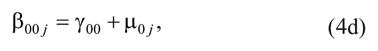


with

where D1 ij and D2 ij were dummy variables to represent the three different subpopulations (i.e., D1 ij = 1 and D2 ij = 0 for Subpopulation A; D1 ij = 0 and D2 ij = 1 for Subpopulation B; and D1 ij = 0 and D2 ij = 0 for Subpopulation C).
The average growth models for the three subpopulations were specified so that the two subpopulations in Study 1 remained the same as in Equations 2a and 2b, and a third subpopulation with a high start but a decelerating mean growth trajectory (i.e., Equation 3k) was added:
Subpopulation C:

We chose the growth pattern for Subpopulation C based on a review by Tofighi and Enders (2008). The shape of estimated growth trajectories usually includes three classes: (a) a “zero class” of individuals with low and stable levels of some problem behaviors (i.e., Subpopulation A), (b) an “accelerating class” with low start but increasing number of problems (i.e., Subpopulation B), and (c) a “decelerating class” with higher start but decreasing number of problems (i.e., Subpopulation C).
Based on the settings presented in Equations 2a, 2b, and 3k and the coding of the dummy variables,
The three subpopulations’ mixing proportions were fixed to be balanced, with 33.33% for each subpopulation, because the effect of mixing proportions was not substantial according to Study 1’s findings. The cluster size was set to be 21 and 42 for the ease of assigning equal number of individuals into three subpopulations during data generation through SAS (version 9.2; SAS Institute Inc., 2002-2008). Because the impact of cluster number has been clearly shown in Study 1, we only adopted the low and high levels for this design factor (i.e., 30 and 80) and omitted the intermediate level (i.e., 50) to reduce the total number conditions. The variances and covariance of the random effects as well as the number of repeated measures were the same as in Study 1. The mean growth trajectories of the three subpopulations and the level of separation under the small and medium

Mean growth trajectories with error bars for small

Mean growth trajectories with error bars for medium
In summary, the simulation used a 2 (magnitude of the
Analyses and Results
The analysis procedures and observed outcomes were the same as those for Study 1. The performance of the six fit indices had several similarities with those in Study 1. Therefore, we only highlighted patterns that are different.
Overall fit index performance
Results including the percentages of correct and incorrect classifications by the six model selection indices for both the true and misspecified models are presented in Figure 7. Because Study 2 contained fewer design conditions than Study 1, only results from design conditions similar across two studies were used for comparison. AIC had a much lower class enumeration accuracy (below 40%) compared with that in Study 1 (above 65%) for both true and misspecified models. CAIC and BIC still performed well in true models; furthermore, their enumeration accuracy under the misspecified models improved by 13% and 11%, respectively, compared with that in Study 1. Compared with results from Study 1, SABIC’s accuracy decreased by 16% under the true model and 7% under the misspecified model, with the overextraction rate increasing by 6% and 4%, respectively. The accuracy of VLMR and ALMR dropped by 7% under the true model and 10% under the misspecified model compared with that in Study 1.
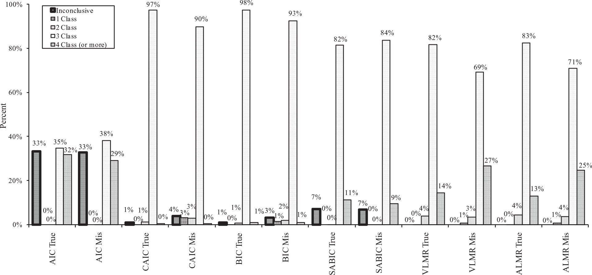
Percentage of one-, two-, three-, four-class (or more) models and inconclusive classification identified by AIC, CAIC, BIC, SABIC, VLMR, and ALMR under true and misspecified models.
In summary, under the misspecified model, BIC and CAIC had higher percentages of correct class enumeration (i.e., 93% and 90%) than SABIC (84%), followed by VLMR and ALMR (69% and 71%). The difference in classification accuracy between true and misspecified models was −2%, −3%, 5%, 8%, 12%, and 12% for SABIC, AIC, BIC, CAIC, ALMR, and VLMR, respectively.
Effect of design factors
The effects of the design factors remained mostly similar as what was found in Study 1; therefore, only a few different patterns are highlighted here. For AIC, cluster number and cluster size affected the classification accuracy negatively (
Study 3: Complex Model in Two-Class Case
In the first two simulation studies, the within-class covariance structure (i.e., the
As expected, there were more convergence issues as the model became more complex. A total of 33 replications were excluded from further analysis due to nonconvergence or local solutions for the three-class MGMM or GMM models. We highlighted the results that are different from Study 1 in the following section (see Table 3). AIC’s accuracy decreased substantially, whereas CAIC, BIC, VLMR, and ALMR became more accurate as the model became more complex. SABIC performed similarly as in Study 1, except its accuracy decreased under the small sample size condition under the true model.
Discussion and Conclusion
The current study examined model selection index performance in class enumeration for MGMMs when the top level of nesting was ignored. As expected, under the correctly specified MGMM, the indices’ performance was mostly consistent with the findings in previous studies. BIC and CAIC had the highest class enumeration accuracy, followed by SABIC, ALMR, and VLMR, with ALMR and VLMR performing similarly. AIC had the lowest enumeration accuracy. SABIC, ALMR, VLRM, and AIC tended to overextract the number of classes when there were three subpopulations and less clear-cut class separation. When the highest data level was ignored and a single-level GMM was fitted to the data, the classification accuracy of all model selection indices decreased compared with the accuracy under the true model. We discuss the impact of design factors, Bonferroni correction with VLMR/ALMR, and the implications for researchers in the following section.
Impact of Design Factors
The impact of ICC
The ICC had the biggest impact on the difference between the true and misspecified models. An important advantage of using multilevel models is that by modeling the higher level nesting structure (e.g., schools), variation in the individual growth trajectories can be decomposed into within- and between-organization components (Raudenbush & Bryk, 2002). As shown in some previous studies on multilevel analysis (e.g., Meyers & Beretvas, 2006; Moerbeek, 2004), ignoring the highest level data structure results in the redistribution of the variance from the ignored level (or the organization/school level) to the adjacent level (i.e., the individual/student level). A similar variance redistribution mechanism has been found in MGMM (e.g., the overestimation of
The impact of degree of separation
The magnitude of the
The impact of sample size
Sample sizes affected the indices in different ways. Our finding is consistent with previous findings that CAIC and BIC tend to select the correct class solution more frequently as sample size increases under the true model (Nylund et al., 2007). However, the impact of small sample size on CAIC and BIC under the misspecified GMM is much more serious than its impact under the true model. Previous research on two-level GMM found that BIC and CAIC tended to underextract the number of classes under small sample sizes even when the model was correctly specified. It is possible that the N adjustment is too strong when N is small or Ln is not the optimal function. However, the performances of SABIC (with smaller penalty on N), VLMR, and ALMR were less affected by small sample size conditions. The performance gaps between the true and the misspecified model for SABIC, VLMR, and ALMR were much smaller than those for CAIC and BIC. Therefore, when sample size was small, SABIC, VLMR, and ALMR were generally more accurate than CAIC and BIC under the misspecified model.
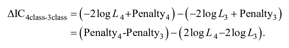
As shown in Equations 1a to 1d, different sample size (N) functions are used in the penalty term for different IC indices. Figure 8 illustrates how class enumeration decisions made by different IC change with sample size based on the log-likelihood values from an empirical data analysis. Suppose we are comparing the three-class solution and the four-class solution. The difference between
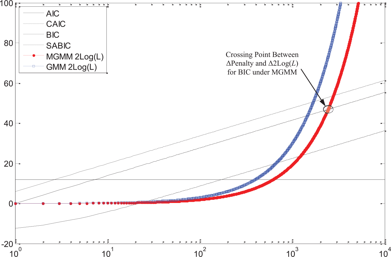
Example of the effect of sample size on class enumeration decisions by IC indices.
Let
Figure 8 shows that when sample size is large enough, all indices will favor the four-class solution. Note that SABIC will also favor the four-class solution when sample size is very small because it has two crossing points. The range of sample size in which the IC indices will select the three-class solution (i.e., when the ∆
The MGMM examined in this study was strategically specified to have only one Level 3 random effect, which captures the intercept variance between cluster/organization means. Under specifications where the number of parameters at Level 3 increases (e.g., by including a slope residual variance, latent classes, or fixed effects at the organization level), ∆
Bonferroni Corrections With VLMR/ALMR
One reason for VLMR/ALMR’s overextracting the number of classes might be increased Type I error rate resulting from multiple testing for the same dataset. In previous research, no correction for α was used and the effect of using corrected α is unknown (B. Muthén, personal communication, March 8, 2011). Therefore, we have examined the accuracy of VLMR and ALMR after applying Bonferroni correction to α in both studies. Based on the number of VLMR/ALMR from each study, we used α = .05 / 2 = .025 for Study 1 and α = .05 / 3 = .167 for Study 2. We found that the overall accuracy of VLMR and ALMR improved under both the true and misspecified models (improvement ranged from 1% to 10%). Furthermore, the difference between the nonadjusted and adjusted VLMR/ALMR increased as the cluster number and cluster size increased. By using the Bonferroni correction to α, VLMR/ALMR is less likely to overextract the number of classes, an improvement especially noticeable in large sample size conditions, in misspecified models, and when there were more than two subpopulations in data generation. There was no appreciable difference between the nonadjusted and adjusted VLMR/ALMR under the small sample size condition (i.e., N = 600 or 630) and for the true model. Therefore, Bonferroni correction seems more appropriate for data with large sample sizes (N ≥ 1,000) only; besides, when the higher level nesting structure is ignored, the Bonferroni correction would be especially useful to achieve higher accuracy for VLMR/ALMR.
Implications for Researchers
Techniques such as GMM and MGMM that are rooted in structural equation modeling can be viewed as model-building techniques in which researchers start with a simpler model and build up to a more complex one (Kline, 2010). The results of the current study can aid researchers in this model-building process because they demonstrate the importance of accounting for nested data structure and provide information on which fit indices can most accurately identify the appropriate model when using MGMM. Based on our findings, we strongly recommend that researchers accommodate multilevel structure by using MGMMs, especially when the sample size is relatively small, the ICC is relatively large, or both. Table 4 summarizes the top performing indices under different conditions.
Better Performing Indices Under Small and Large N by Type of Model.

Note. MGMM = multilevel growth mixture model; SABIC = sample size–adjusted BIC; BIC = Bayesian information criterion; CAIC = consistent AIC; VLMR = Vuong–Lo–Mendell–Rubin likelihood ratio test; ALMR = adjusted Lo–Mendell–Rubin likelihood ratio test; GMM = growth mixture model; AIC = Akaike information criterion.
In general, when the sample size is small, SABIC is preferred, whereas when the sample size is large, BIC and CAIC are preferred. Note that the sample size is relative to ICC. For example, 1,200 may be considered as a large sample size when ICC is .1, but small when ICC is .2.
The cutoff value of 2 is a reasonable value to use for BIC, CAIC, and SABIC. In the process of finding the best fit model, when the decrease in the indices’ values (especially SABIC) becomes less than 2, researchers can stop fitting more complicated models (i.e., models with more classes) and select the model with the second lowest IC index.
VLMR and ALMR can be used as references when sample size is small (i.e., N ≤ 630), but should be used with caution when sample size is large due to their tendency to overextract classes. Bonferroni correction can help improve VLMR/ALMR’s accuracy for data with large sample size (N ≥ 1,000).
Under more complex models, we recommend using CAIC, BIC, VLMR, and ALMR for MGMM; SABIC is only suitable for large sample size conditions. For misspecified models, CAIC and BIC are best, SABIC is appropriate for large sample size conditions, and VLMR and ALMR can also be used, but tend to overextract classes.
It is important to note that these fit index recommendations are based on the simulation conditions used in this study. Readers should be cautious when applying our findings to models and conditions that are very different from those studied in this article.
Limitations and Future Directions
Accurate class enumeration is perhaps the greatest challenge in mixture modeling and much is still unknown about highly complex mixture models such as the MGMM. That said, there are some limitations to the current study that raise caution regarding generalizing the results. First, the residual variance of the slope at the organization level was constrained to zero. While this specification will be common for empirical studies because organization level slope variation tends to be small, which may result in convergence problems (Palardy & Vermunt, 2010), including the organization level slope random effect and other Level 3 parameters may impact class enumeration.
Second, while this study focuses on the particular model misspecification of ignoring the highest level of the hierarchical data, there are other types of model misspecifications and assumption violations that may affect class enumeration. For instance, misspecifying the shape of the growth trajectory or violating the multivariate normality assumption for the repeated measures can effect class enumeration (Bauer & Curran, 2003, 2004). Additional research is needed to address these issues.
Third, the current study was conducted under frequentist estimation using the maximum likelihood estimator. Recently, Bayesian estimation for multilevel models has been gaining attention due to its advantages over the classical approach (Hamaker & Klugkist, 2011). The deviance information criterion (DIC; Spiegelhalter, Best, Carlin, & Van der Linde, 2002) is available under the Bayesian estimation, and it can be used in similar fashion as the AIC and BIC to select the optimal model (i.e., models with small DIC values are favored). In the most recent version of Mplus 6.1 (L. K. Muthén & Muthén, 1998-2010), the Bayesian estimator is available but not yet implemented for MGMM (B. Muthén, personal communication, July 29, 2011). In addition, Bayesian analysis with a specific prior distribution allows model selection using posterior model probabilities or the Bayes factor (Hamaker & Klugkist, 2011). We expect the model selection by DIC to be similar to AIC according to Spiegelhalter et al. (2002), whereas Bayes factor and posterior probabilities under full Bayesian analysis to be similar to the BIC, as they belong to Bayesian model selection approach. Additional research on the performance of DIC, posterior model probabilities, and Bayes factor for MGMM and GMM under the Bayesian estimation framework is needed to see how they compare with the classical/frequentist approach.
Footnotes
Appendix
Below is a list of all acronyms used in the current article as well as what they denote, in alphabetical order.
AIC—Akaike information criterion
ALMR—adjusted Lo–Mendell–Rubin likelihood ratio test
ANOVA—analysis of variance
BIC—Bayesian information criterion
BLRT—bootstrap likelihood ratio test
CAIC—consistent Akaike information criterion
FMM—factor mixture model
GMM—growth mixture model
IC—information criterion
ICC—intraclass correlation
ID—identifier
IRT—item response theory
LCA—latent class analysis
LCGA—latent class growth model
LGCM—latent growth curve model
LR—likelihood ratio
LRT—likelihood ratio test
K-L—Kullback–Leibler
MGMM—multilevel growth mixture model
SABIC—sample size–adjusted BIC
VLMR—Vuong–Lo–Mendell–Rubin likelihood ratio test
Declaration of Conflicting Interests
The author(s) declared no potential conflicts of interest with respect to the research, authorship, and/or publication of this article.
Funding
The author(s) received no financial support for the research, authorship, and/or publication of this article.