Sage Journals: Discover world-class research

Abstract

The most common effect size when using a multiple-group confirmatory factor analysis approach to measurement invariance is ΔCFI and ΔTLI with a cutoff value of 0.01. However, this recommended cutoff value may not be ubiquitously appropriate and may be of limited application for some tests (e.g., measures using dichotomous items or different estimation methods, sample sizes, or model complexity). Moreover, prior cutoff value estimations often have ignored consequences resulting in using measures that more accurately estimate countries’ or learners’ proficiency for some countries or groups versus others. In this study, we investigate whether the cutoff value proposed by Cheung and Rensvold (ΔCFI or ΔTLI > 0.01) is appropriate across educational measurement contexts. Specifically, we investigated the performance of ΔCFI and ΔTLI in capturing LOI at the scalar level in dichotomous items within item response theory on groups whose test characteristic curves differed by 0.5. Simulation results showed that the proposed cutoff value of 0.01 in ΔCFI and ΔTLI was not appropriate to capture LOI under the study conditions, which may result in the misinterpretation of test results or inaccurate inferences.

Keywords

measurement invariance differential item functioning scalar invariance multiple-group confirmatory factor analysis

Introduction

A desirable property of a measurement instrument is that individuals with the same measurement scores should have the same standing on the construct measured by the instrument (Millsap, 2012; Schmitt & Kuljanin, 2008). Stated mathematically, the distribution of the observed scores Y should be a function of the trait η and independent of the irrelevant construct s (Millsap, 2012):

f (Y | η, s) = f (Y | η)

(1)

In social sciences, measurement invariance is studied on a set of items administered to people from different groups, such as race, gender, or age, and it is expected that those items should behave the same across those groups (Wells, 2021). Establishing measurement invariance (MI) is part of evaluating measurement quality and accuracy. Violation of MI assumptions threatens the substantive interpretation of the observed scores (Vandenberg & Lance, 2000). Measurement non-invariance or lack of invariance (LOI) is a type of systematic error introduced in the relationship between the latent factor and the manifest indicator (Vandenberg & Lance, 2000). One commonly used method within structural equation modeling (SEM) framework to assess MI is multiple group confirmatory factor analysis (MG-CFA). Within MG-CFA, one general criterion to determine LOI is the magnitude of change in comparative fit index (CFI) or Tucker–Lewis index (TLI) across hierarchically constrained nested models. Cheung and Rensvold’s (2002) proposed change of a ΔCFI or ΔTLI >0.01 has been widely used in the applied SEM literature and operational psychometrics as a cutoff value to flag LOI.

There are several limitations on the proposed cutoff values, however. First, the cutoff values have been recommended without considering the context and the purpose of the assessment or in a context that differs from large-scale educational assessments as the ones we consider in this article. For example, previous studies in this area have examined MI for indicators that are based on many categories where the items are treated as continuous. However, large-scale educational tests or questionnaires in quality-of-life evaluation are often comprised of multiple-choice items that are categorically (e.g., dichotomously) scored.

Second, when developing cutoff values, previous studies have ignored the consequences of LOI, and questions such as whether the presence of LOI would lead to practically important consequences have been left unexamined. The importance of examining consequences using large-scale educational tests has been highlighted in Oliveri et al. (2018). The authors explain that examining consequences of educational tests is critical to the meaningful use of such assessments. Because large-scale educational tests are used to make important decisions related to educational policy and practice, resource allocation, and comparisons in performance across groups, the identification of cutoff values that work well within our focal type of tests is important. In addition, consequences of measurement invariance violation manifest in other fields, such as in racial equity in health services. The study of the lack of measurement invariance is a significant opportunity to advance the way we measure health inequalities with a particular focus on race differences. It is crucial to evaluate the assumptions that guide quantitative associations with health variables, and racial equity in the policy options that are considered as a result of quantitative findings. Psychometric work can help us better understand whether there are potential race differences in the concept under study so that we can develop new measures or correct existing ones. Without such investigations, threats to validity may be introduced through overlooked cross-cultural differences among groups, which may threaten valid score interpretation. To elaborate, Oliveri and von Davier (2017) pointed out that when assessments are administered internationally, such as with the Program for International Student Assessment (PISA) administered across countries, LOI may emerge in relation to differential exposure to the item types used in PISA, how close the participating countries’ language is to the original language in which the tests were developed, and differences in exposure to the curricula or difference in opportunity to learn across countries or groups within countries. Because DIF is used as a step to flag this type of differences, accurate estimation of DIF is important when using educational tests.

One way of statistically measuring the effect of consequences is through the impact of MI on test scores. For example, if the MI resulted in examinees with the same proficiency but from different groups (e.g., based on testing mode, gender, or race) received a sufficiently different expected raw score, then the MI may result in consequences such as differential ranking of examinees based on test scores, differential admission rates for some groups versus others, or adverse impact in the use of tests for employment or hiring purposes.

In the present study, non-negligible LOI was operationally defined as the difference in expected raw scores equal to 0.5 on the item response theory (IRT) scale. The difference in the expected raw scores can be determined by comparing test characteristic curves (TCC) across groups within an IRT framework. In this study, non-negligible LOI was operationally defined as the difference in the TCCs between two groups equal to 0.5 for any proficiency value. The rationale for the selection of a TCC difference of 0.5 is that such a difference would result in a one-point difference in raw score due to rounding error.

Third, although previous studies have examined several fit indices across multiple conditions, they have not addressed the effect of several important factors (including the percentage of LOI items, the IRT model used, the values of the a and b parameter values, and the sample sizes used in the simulation) on the change in fit indices when determining an appropriate cutoff value. For example, is the change in fit indices (e.g., ΔCFI) influenced by item discrimination? Therefore, one of the purposes of the present study is to examine the impact of several important factors that may influence the distribution of the change in fit indices in assessing MI.

To address these three major limitations of previous studies, the present research employs a simulation to (a) evaluate the appropriateness of the proposed cutoff value of ΔCFI and ΔTLI >0.01 (Cheung & Rensvold, 2002) in an educational measurement context, and (b) examine the effects of several relevant factors on the change of fit indices for assessing MI using MG-CFA (the percentage of LOI items, the IRT model used, the values of the a and b parameter values, and the sample sizes used in the simulation). This exploration is not new as several studies (e.g., Jin, 2020; Khojasteh & Lo, 2015; Sass et al., 2014) have shown that Cheung and Rensvold’s (2002) general cutoff value may not be appropriate in certain measurement design conditions. The present study further corroborates the findings of the foregoing authors by introducing a priori non-negligible LOI. In the present study, it is hypothesized that Cheung and Rensvold’s (2002) proposed cutoff values of a ΔCFI and ΔTLI >0.01 is not applicable to dichotomous items under study conditions.

To address these objectives, first an overview of MI and the MG-CFA approach to evaluating LOI is presented. Then, a description of the relevant fit indices commonly used in MG-CFA will be provided. Next, our simulation study in which we describe how we evaluated Cheung and Rensvold’s (2002) proposed cutoff value in the presence of a predetermined 0.5 TCC difference will be presented. The paper is concluded by presenting the results, implications, and future research recommendations.

Measurement Invariance and Multiple-Group Confirmatory Factor Analysis

MG-CFA is an extension of the common factor CFA. It is one of the most frequently used methods in assessing MI in applied research and operational measurement (Schmitt & Kuljanin, 2008). In the MG-CFA framework, to establish MI, different (nested) tests are conducted, each testing one aspect of the measurement model, which is based on the following two equations:

X_{k}^{g} = τ_{k}^{g} + Λ_{k}^{g} ξ^{g} + δ_{k}^{g}

(2)

Σ^{g} = Λ_{X}^{g} Φ^{g} Λ_{X}^{g'} + Θ_{δ}^{g}

(3)

where $X_{k}^{g}$ refers to the vector of item responses 1, …, k, in group g, $τ_{k}^{g}$ is the vector of regression intercepts, $Λ_{k}^{g}$ refers to the matrix of regression slopes, $ξ^{g}$ is the common factor, $δ_{k}^{g}$ refers to the vector of unique factors, $Σ^{g}$ refers to the variance-covariance matrix among the k items in each group, $Λ_{X}^{g}$ refers to the matrix of factor loadings, $Φ^{g}$ is the variance-covariance matrix for inter-factor relationship, and $Θ_{δ}^{g}$ is the diagonal matrix of unique variances.

Based on the number of parameters being estimated, eight different invariance tests can be performed, of which the first five assess MI (relationships between measured variables and latent factors); the last three test structural invariance (tests about latent factors themselves; Byrne et al., 1989; Schmitt & Kuljanin, 2008). Because in this study we are concerned only with MI, only the first four tests are briefly elaborated below.

Covariance Matrix Invariance

In this equality test, the researcher attempts to establish the conditional equality of the variance-covariance matrices derived from the different subpopulations. Failure to reject the null hypothesis that $Σ^{g} = Σ^{g'}$ shows the equality of measurement equivalence and allows the researcher to dispense with further MI tests.

Configural Invariance

In this equality test, the goal is to establish the equality of the factor structure across groups. The null hypothesis is that the a priori pattern of free and fixed factor loadings is equal across groups.

Metric Invariance

In this equality test, the aim is to establish the equality of the factor loadings across groups. In the metric invariance analysis, one indicator factor loading is fixed to 1 as a referent indicator and regarded invariant.

Scalar Invariance

In this equality test, we test if the vector of item intercepts or thresholds are invariant across groups. In psychometrics literature, scalar non-invariance is also known as differential item functioning (DIF). In this article, we use DIF and scalar LOI interchangeably. If scalar invariance is established, any differences in observed scores between groups can be attributed to their differential constructs (Millsap & Olivera-Aguilar, 2012). This test also allows the establishment of the equality of factor means across groups (Schmitt & Kuljanin, 2008).

CFA Model Fit Indices

The root mean squared error of approximation (RMSEA; Steiger, 1990), comparative fit index (CFI), and Tucker-Lewis index (TLI) are some of the most common fit indices used to interpret CFA fit results. These fit indices are also used in assessing MI.

RMSEA is a standardized index that indicates the degree of agreement or discrepancy between the observed (empirical) and model-based (theoretical) item characteristic curves. A value of zero indicates a perfect model-data fit because there are no differences between the empirical and theoretical item characteristic curves. Higher RMSEA values indicate poorer model-data fit estimates because there are larger gaps between the model and observed item characteristic curves. The RMSEA is parsimony-adjusted measure of model discrepancy in the population and is computed as,

ε = \sqrt{\frac{δ}{df (N - 1)}}

(4)

where δ is the non-centrality parameter, df is the degree of freedom, and N is the sample size. δ is defined as follows:

δ = \max (χ^{2} - df, 0)

(5)

RMSEA penalizes free parameters through dividing them by df. It also rewards a large sample size because N is in the denominator. Previous research has adopted an RMSEA value of 0.1 as indicative of fit (Oliveri & von Davier, 2014, 2017).

CFI is another model discrepancy fit index based on the non-centrality measure that compares the fit of the model with a baseline (independence) model. CFI is derived as:

CFI = 1 - \frac{{\hat{δ}}_{M}}{{\hat{δ}}_{B}}

(6)

The δ’s are calculated for the researcher’s model (M) and the baseline or null model (B). The baseline model is a null or independence model in which the covariances among all input indicators are fixed to zero. A CFI >0.95 is commonly used to indicate good fit (Brown, 2006; Hu & Bentler, 1999).

TLI is another model discrepancy fit index which compares the fit between the target and baseline models, which is calculated as follows:

TLI = \frac{\frac{χ_{B}^{2}}{d f_{B}} - \frac{χ_{M}^{2}}{d f_{M}}}{\frac{χ_{B}^{2}}{d f_{B}} - 1}

(7)

TLI is a function of the average correlation among the indicators. A TLI > .95 is commonly used to indicate good fit (Brown, 2006; Hu & Bentler, 1999).

Present Study

In this study, MG-CFA was used to investigate the performance of the CFI, TLI, and the RMSEA model fit indices in detecting scalar non-invariance in the presence of non-negligible MI induced by 0.5 difference in test characteristic curve (TCC) between the focal and the reference groups on a simulated one-dimensional IRT-calibrated test with 40 dichotomous items. The purpose of the study was to evaluate the appropriateness of Cheung and Rensvold’s (2002) proposed effect size criterion (ΔCFI > 0.01) in capturing scalar invariance when the items are dichotomous and parameters are estimated using robust weighted least squares. In addition, the effect of five factors on change in the CFI, TLI, and the RMSEA model fit indices was investigated, including the percentage of DIF items (10% and 20%), IRT model used (2PL and 3PL), the a (0.5, 1.0, and 1.5) and the b (−1 and 0, 1) parameter values, and the sample size (500, 1,000, and 2,000). Overall, 108 conditions were simulated and investigated.

Data Generation

Dichotomous item responses were generated for a 40-item test under five crossed factors: IRT models (2PL and 3PL), percentage of LOI items (10% and 20%), the a-parameter value for DIF items (0.5, 1.0, and 1.5), the b-parameter value for LOI items (−1, 0, and 1), and sample size per group (500, 1,000, and 2,000 responses).

To generate the item responses, two IRT models were used: the 3PL and the 2PL models. The 3PL model specifies the probability of a correct response given three item characteristics and a person parameter, and is formulated as the following logistic function:

P (θ_{j}) = c_{i} + (1 - c_{i}) \frac{e^{1.7 a_{i} (θ_{j} - b_{i})}}{1 + e^{1.7 a_{i} (θ_{j} - b_{i})}}

(8)

where b represents the item difficulty, a represents the item discrimination, and c represents the pseudo-guessing parameter. The 2PL model dispenses with the c parameter.

To generate responses, parameters from a real proficiency test were used. In order to produce new parameters for the DIF items, parameters in the focal group were manipulated for each fixed parameter of the reference group.

The simulation steps for the present study proceeded as follows:

Item parameters estimated through an IRT model from a real test were obtained. The 40-item parameters were duplicated, one set for the reference group and the other set for the focal group. Previous research has similarly been conducted using a fixed test length of 40 binary items and calibrated IRT-based parameters using an educational test (Oliveri et al., 2013, 2014).

Each study condition was set according to the a and the b parameter values, the number of DIF items, the IRT model, and the sample size (108 conditions).

Once the parameters for a study condition were set, the value of the b parameter was manipulated only in the focal group to produce an amount of LOI that resulted in a 0.5 difference TCC value between the reference and the focal groups.

Next, item responses were simulated based on the changed parameter values in the original 40-item sets.

Finally, the obtained item responses were used in the Mplus (Muthén & Muthén, 2015) software for MG-CFA study to investigate the effect of different conditions on the obtained effect sizes (CFI, TLI, and RMSEA).

Table A1 in Appendix A shows different b values in the focal group used to simulate DIF items for different conditions.

Before proceeding to examine the distributions for each of the changes in goodness-of-fit indices, the Mantel-Haenszel (MH) DIF procedure was used to flag items for a few select conditions to ensure the data were generated appropriately. If the simulation was correct, we expected the DIF items to be flagged at a much higher rate than the non-DIF items and the average effect size to be greater for the DIF items compared to the non-DIF items. Also, we expected the non-DIF items not to be flagged much beyond a nominal alpha level of .05. The MH DIF procedure was applied to three conditions where the a parameter varied (i.e., a = 0.5, 1.0, and 1.5) when generating data using the 2PLM and a sample size of 1,000. Table A2 in Appendix A shows the proportion of replications that each simulated DIF item was flagged as DIF and the mean effect size, ΔMH for the selected conditions. Because the MH DIF method was able to detect the DIF items with reasonable power, it seems that the items were generated appropriately. Furthermore, the average ΔMH across the items was reasonably large for all of the DIF items.

Model Fitting

Sequential equality constraints were imposed on factor structure, factor loadings, and indicator thresholds for the purpose of testing measurement invariance at configural, metric, and scalar levels, respectively, and calculated sequential differences in CFI, TLI, and the RMSEA fit indices. Parameters were estimated using the Mplus software (Muthén & Muthén, 2015) using robust diagonally weighted least squares (WLSMV) estimation method (Muthén et al., 1997). One non-DIF item was selected as the referent indicator for scaling the latent variable in both groups.

Data Analysis

The mean, standard deviation, skewness, and kurtosis for each fit index change (ΔCFI, ΔTLI, and ΔRMSEA) for 1,000 replications were calculated. In addition, a five-way ANOVA was run to determine the important factors that may have influenced the means of the distributions. An effect size based on partial eta-squared was used to identify effects that were practically meaningful. Because the conditions were the same with respect to the consequences of including LOI in the assessment, for the fit indices to be useful, their expected value should remain the same across the conditions.

Results

Performance of ΔCFI, ΔTLI, and ΔRMSEA

Table 1 includes change values in CFI, TLI, and RMSEA fit indices for sample size 500 and the 3PL IRT model. Although the MH test procedure showed the presence of DIF items in the simulated test scores, the CFI, TLI, and the RMSEA fit indices seem to fail in capturing model fit deterioration due to the existence of measurement non-invariance at the scalar level. As the different fit index change values show, they are much smaller than the recommended 0.01 cutoff value suggested by Cheung and Rensvold (2002). At a given value of b, we can see that as the a parameter increases, the changes in both the CFI and the TLI become smaller, indicating the offsetting contribution of the a parameter in the presence of DIF. A similar change can also be observed for the RMSEA index. For instance, at b = 0, the RMSEA change decreases from 0.005 to 0.003 and to 0.001 for a parameter values of 0.5, 1.0, and 1.5, respectively. However, the change is positive, which is unexpected. We do not see any noticeable change from one condition to another. However, change is largest at the lowest level of the discrimination parameter. This once again shows the offsetting role of the a parameter in the presence of DIF.

Table 1.

Change in Equal Loadings Equal Threshold (Scalar Invariance) CFI, TLI, and RMSEA Across Conditions for N = 500 and IRT = 3PL.

Percent DIF (%)	Index	b = −1			b = 0			b = 1
Percent DIF (%)	Index	a = 0.5	a = 1.0	a = 1.5	a = 0.5	a = 1.0	a = 1.5	a = 0.5	a = 1.0	a = 1.5
10	CFI	−0.002	−0.001	−0.000	−0.003	−0.001	−0.000	−0.002	−0.001	−0.000
	TLI	−0.003	−0.001	−0.000	−0.003	−0.002	−0.000	−0.003	−0.001	−0.000
	RMSEA	0.007	−0.001	0.001	0.005	0.003	0.001	0.004	0.002	0.001
20	CFI	−0.001	−0.000	−0.000	−0.001	−0.000	−0.000	−0.001	−0.000	−0.000
	TLI	−0.001	−0.000	−0.000	−0.001	−0.000	−0.000	−0.001	−0.000	−0.000
	RMSEA	0.001	0.000	0.000	0.001	0.000	0.000	0.001	0.000	0.000

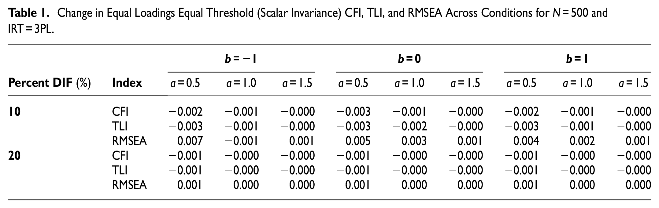
Table 2 shows the results of simulation when the sample size increased to 1,000, and the IRT model was the 3PL. A close examination of Table 2 confirms the effect of the a parameter value on the magnitude of the CFI, TLI, and RMSEA changes, especially on the TLI. The changes are more pronounced when the percentage of DIF is 10%. When the percentage of DIF increases to 20%, we can see that the small changes are consistent across conditions except for the TLI index. One interesting pattern in these observations is the CFI, TLI, and the RMSEA changes at DIF = 20%, b = 0 and a = 1.5. Only in this condition do these fit indices reflect the change associated with scalar invariance similar to the Cheung and Rensvold’s (2002) recommended threshold of 0.01. Nevertheless, we can arrive at the same conclusion that none of these fit indices were able to capture the simulated scalar non-invariance, questioning the appropriateness of the cutoff value of 0.01 in all measurement settings.

Table 2.

Change in Equal Loadings Equal Threshold (Scalar Invariance) GFI’s Across Conditions for N = 1,000 and IRT = 3PL.

Percent DIF (%)	Index	b = −1			b = 0			b = 1
Percent DIF (%)	Index	a = 0.5	a = 1.0	a = 1.5	a = 0.5	a = 1.0	a = 1.5	a = 0.5	a = 1.0	a = 1.5
10	CFI	−0.001	−0.000	0.000	−0.001	−0.000	0.000	−0.000	−0.000	−0.000
	TLI	−0.005	−0.002	−0.001	−0.005	−0.003	−0.001	−0.004	−0.001	−0.000
	RMSEA	0.001	0.000	0.000	0.001	0.000	0.000	0.001	0.000	0.000
20	CFI	−0.000	0.000	0.000	−0.000	0.000	−0.011	−0.000	0.000	0.000
	TLI	−0.002	−0.001	0.000	−0.002	−0.000	−0.012	−0.001	0.001	0.001
	RMSEA	0.000	0.000	0.000	0.000	0.000	0.010	0.000	0.000	−0.000

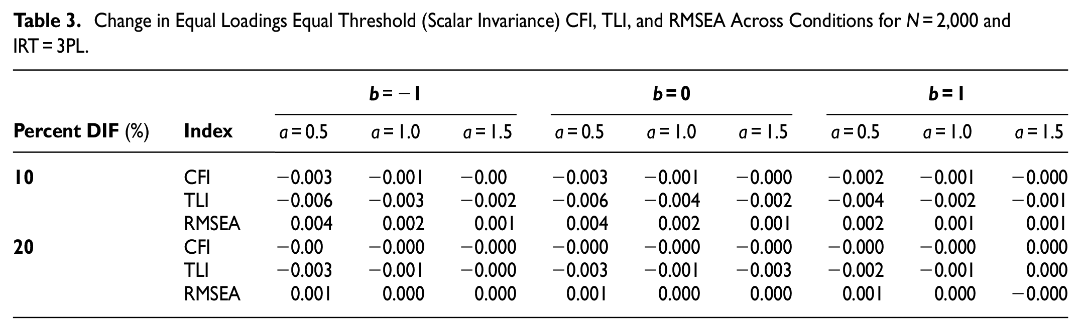
Table 3 exhibits the simulation results for sample size 2,000 and the 3PL IRT model. Similar to the results in other sample sizes, the effect of the a parameter on the changes in fit indices is present. The unrevealing changes in the fit indices show that they have failed to capture the simulated scalar non-invariance in the data.

Table 3.

Change in Equal Loadings Equal Threshold (Scalar Invariance) CFI, TLI, and RMSEA Across Conditions for N = 2,000 and IRT = 3PL.

Percent DIF (%)	Index	b = −1			b = 0			b = 1
Percent DIF (%)	Index	a = 0.5	a = 1.0	a = 1.5	a = 0.5	a = 1.0	a = 1.5	a = 0.5	a = 1.0	a = 1.5
10	CFI	−0.003	−0.001	−0.00	−0.003	−0.001	−0.000	−0.002	−0.001	−0.000
	TLI	−0.006	−0.003	−0.002	−0.006	−0.004	−0.002	−0.004	−0.002	−0.001
	RMSEA	0.004	0.002	0.001	0.004	0.002	0.001	0.002	0.001	0.001
20	CFI	−0.00	−0.000	−0.000	−0.000	−0.000	−0.000	−0.000	−0.000	0.000
	TLI	−0.003	−0.001	−0.000	−0.003	−0.001	−0.003	−0.002	−0.001	0.000
	RMSEA	0.001	0.000	0.000	0.001	0.000	0.000	0.001	0.000	−0.000

Similar results were obtained with the 2PL IRT, showing that the change in CFI/TLI fit indices was much lower than the commonly used 0.01 threshold for assessing MI (see Tables A3 –A5 in Appendix A for the simulation results for the 2PL IRT model.)

ANOVA Results

A five-way ANOVA was performed to investigate if there were any differences between the factors in terms of their effect on the amount of change in each fit index. ANOVA Table 4 shows that the differences were statistically significant, though it is more appropriate to refer to the partial eta squared values to evaluate the effect of the factors and their interactions. Relying on effect size statistic, only factors and interactions with a partial eta squared value ≥.06 are included in the following table (ANOVA tables for change in TLI and RMSEA are provided in the online supplement).

Table 4.

Five-Way ANOVA on CFI Change Across the Five Factors.

Source of variation	Sum of squares	df	Mean square	F	p	Partial eta squared
Sample size	0.007	2	0.003	3,145.0	<.001	.06
IRT model × percent DIF	0.009	1	0.009	8,262.1	<.001	.07
IRT model × parameter “ a ”	0.009	2	0.004	4,153.3	<.001	.07
Percent DIF × parameter “ a ”	0.007	2	0.003	3,207.9	<.001	.06
Sample size × parameter “ a ” × parameter “ b ”	0.009	8	0.001	1,011.4	<.001	.07
Sample size × IRT model × percent DIF × parameter “ a ”	0.008	4	0.002	1,799.4	<.001	.07
Sample size × IRT model × parameter “ a ” × parameter “ b ”	0.009	8	0.001	1,105.4	<.001	.08
Sample size × percent DIF × parameter “ a ” × parameter “ b ”	0.010	8	0.001	1,107.0	<.001	.08
Sample size × IRT model × percent DIF × parameter “ a ” × parameter “ b ”	0.009	8	0.001	1,017.2	<.001	.07
Error	0.116	107,892	<0.001
Total	0.297	107,999

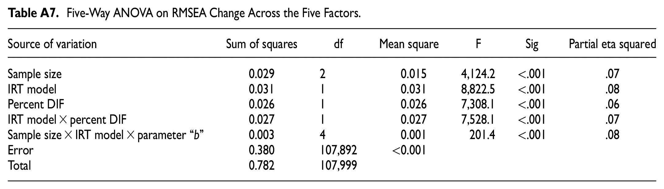
The results of ANOVA on the TLI and RMSEA are presented in Tables A6 and A7 in Appendix A.

Discussion

In the CFA framework, a commonly suggested criterion used to evaluate MI is ΔCFI (or ΔTLI) <0.01 (Cheung & Rensvold, 2002); that is, if the CFI for the invariant model is less than 0.01, then the LOI is considered trivial. This criterion, however, was derived from situations where items were not intended for educational measurement. Several simulation studies (e.g., Jin, 2020; Khojasteh & Lo, 2015; Sass et al., 2014) have shown that Cheung and Rensvold’s (2002) general cutoff value may not be appropriate in certain measurement design conditions.

The results from our research also showed that a cutoff value of 0.01 for ΔCFI or ΔTLI was not appropriate in situations where items are dichotomous and calibrated through an IRT framework. The results of the study showed that although the MH procedure detected the presence of DIF items, using the practical effect size criterion proposed by Cheung and Rensvold (2002) for the CFI and TLI fit indices failed to support the inference that the LOI was non-negligible (i.e., the simulated 0.5 difference between the focal and the reference groups). In other words, one cannot solely rely on the proposed cutoff value in all contexts and under all conditions, as was ostensibly suggested in the results of the present study. Although the MH procedure confirmed the presence of DIF (scalar noninvariance), Cheung and Rensvold’s (2002) cutoff value could not determine a non-trivial LOI.

One explanation could be the small effect from the differences between the values of the b parameters in the focal and the reference groups. Because the difference between the b parameters of the DIF items in the reference and focal groups was dependent on the value of the a parameter, the occurrence of a few DIF items when the a parameters are high may not affect the summary fit indices in the CFA analysis. In the CFA framework, the fit indices are summary statistics and may be influenced by the majority of the item parameters to the effect of missing on the performance of some DIF items. This pattern is seen in this study, where the MH procedure on the individual items can detect the DIF items while summary statistics such as the CFI, TLI, and the RMSEA seem to fail to indicate the characteristics of the study items if the flagging criterion used is that of the Cheung and Rensvold (2002) of ΔCFI >0.01. Therefore, a cutoff value based on summary statistics, such as CFI, TLI, and RMSEA, needs to be determined in the specific measurement context and preferably complimented by other summary statistics and also item-level DIF measures, such MH test, logistic regression, and IRT-based DIF indices.

Future Research

The present study can be expanded in several ways. In the present study, the non-negligible difference in the TCC between the reference and the focus groups was set at 0.5. At this ΔTCC value, the fit indices criteria (particularly the ΔCFI and ΔTLI) failed to detect fit deterioration across the simulated DIF items. Therefore, one interesting factor to take into account in a future study would be to introduce different magnitudes of ΔTCC (e.g., 1.0 and 1.5).

Another factor that may be interesting to investigate is the DIF patterns. In the present study, uniform DIF was simulated to study the behavior of the fit indices and the adequacy of the cutoff value in detecting MI. An advantage of using the IRT estimation framework in this study is that non-uniform DIF patterns can be easily simulated and studied with respect to their effect on model fit indicators. In addition, mixed DIF patterns and their proportion in a set of items can also be simulated and added to the model complexity to evaluate the appropriateness of the present CFI, TLI, and RMSEA criteria in detecting violation of MI.

Items used in the present study were dichotomous. It would be interesting to investigate how the results would be affected if the items were polytomous and estimated through an IRT model. Because in polytomous items more than one b parameter value is estimated, therefore in simulating DIF items and defining a minimally interesting DIF impact different strategies need to be adopted. In the polytomous case, the TCC is calculated as in the dichotomous case but with an additional step. While in dichotomous IRT, the TCC is the sum of the ICC’s, in polytomous IRT the TCC is the sum of the summed ICC of individual categories. So, in conducting a study similar to the present one but on polytomous items, the TCC will be not only a function of simulated thresholds, but also the number of items. This may cause a difficulty if the minimal DIF impact is kept small because one polytomous item could produce that impact and when the study condition requires more than one simulated DIF items, the degree of DIF in thresholds may need to be reduced to achieve the minimally interesting DIF impact.

Because DIF may threaten the accurate and valid interpretation of scores from educational assessments when tests are administered across diverse groups, the investigation of DIF deserves attention. Such investigations are particularly needed when tests are administered across populations with differing abilities, such as higher versus lower performing countries (e.g., such as in the case of PISA and other assessments administered internationally), where one country’s proficiency may be much lower than another country and the validity of any resulting score for a lower performing system could be compromised. Without accurately interpreting the results and controlling LOI, unintended negative consequences may follow from the inaccurate interpretation of tests such as inappropriate allocation of resources or instructional interventions for the most-needy populations. Consequently, additional research on the accurate and appropriate analysis of data from educational tests is needed.

Footnotes

Appendix A

Table A7.

Five-Way ANOVA on RMSEA Change Across the Five Factors.

Source of variation	Sum of squares	df	Mean square	F	Sig	Partial eta squared
Sample size	0.029	2	0.015	4,124.2	<.001	.07
IRT model	0.031	1	0.031	8,822.5	<.001	.08
Percent DIF	0.026	1	0.026	7,308.1	<.001	.06
IRT model × percent DIF	0.027	1	0.027	7,528.1	<.001	.07
Sample size × IRT model × parameter “b”	0.003	4	0.001	201.4	<.001	.08
Error	0.380	107,892	<0.001
Total	0.782	107,999

Declaration of Conflicting Interests

The author(s) declared no potential conflicts of interest with respect to the research, authorship, and/or publication of this article.

Funding

The author(s) received no financial support for the research, authorship, and/or publication of this article.

Ethical Approval

No human or animals used. All data simulated.

ORCID iD

Abdolvahab Khademi

References

Brown

T. A.

(2006). Confirmatory factor analysis for applied research. The Guilford Press.

Byrne

B. M.

Shavelson

R. J.

Muthén

(1989). Testing for the equivalence of factor covariance and mean structures: The issue of partial measurement invariance. Psychological Bulletin, 105, 456–466.

Cheung

G. W.

Rensvold

R. B.

(2002). Evaluating goodness-of-fit indexes for testing measurement invariance. Structural Equation Modeling: A Multidisciplinary Journal, 9(2), 233–255.

Bentler

P. M.

(1999). Cutoff criteria for fit indices in covariance structure analysis: Conventional criteria versus new alternatives. Structural Equation Modeling, A Multidisciplinary Journal, 6(1), 1–55.

Jin

(2020). A note on the cutoff values of alternative fit indices to evaluate measurement invariance for ESEM models. International Journal of Behavioral Development, 44(2), 166–174.

Khojasteh

W. J.

(2015). Investigating the sensitivity of goodness-of-fit indices to detect measurement invariance in a bifactor model. Structural Equation Modeling: A Multidisciplinary Journal, 22(4), 531–541.

Millsap

R. E.

(2012). Statistical approaches to measurement invariance. Routledge.

Millsap

R. E.

Olivera-Aguilar

(2012). Investigating measurement invariance using confirmatory factor analysis. In Hoyle

R. H.

(Ed.). Handbook of structural equation modeling (pp. 380–392). The Guilford Press.

Muthén

du Toit

S. H. C.

Spisic

(1997). Robust inference using weighted least squares and quadratic estimating equations in latent variable modeling with categorical and continuous outcomes (Unpublished Technical Report).

10.

Muthén

L. K.

Muthén

(2015). Mplus: The comprehensive modelling program for applied researchers: User’s guide.

11.

Oliveri

M. E.

Ercikan

Zumbo

B. D.

(2013). Analysis of sources of latent class DIF in international assessments. International Journal of Testing, 13(3), 272–293.

12.

Oliveri

M. E.

Ercikan

Zumbo

B. D.

(2014). Effects of population heterogeneity on accuracy of DIF detection. Applied Measurement in Education, 27(4), 286–300.

13.

Oliveri

M. E.

Rutkowski

(2018). Bridging validity and evaluation to match international largescale assessment claims and country aims (Research Report No. RR-18-27). Educational Testing Service.

14.

Oliveri

M. E.

von Davier

(2014). Towards increasing fairness in score scale calibrations employed in international large-scale assessments. International Journal of Testing, 14(1), 1–21.

15.

Oliveri

M. E.

von Davier

(2017). Analyzing invariance of item parameters used to estimate trends in international large-scale assessments. In Jiao

Lissitz

R. W.

(Eds.), Test fairness in the new generation of large-scale assessment (pp. 121–146). Information Age.

16.

Sass

D. A.

Schmitt

T. A.

Marsh

H. W.

(2014). Evaluating model fit with ordered categorical data within a measurement invariance framework: A comparison of estimators. Structural Equation Modeling: A Multidisciplinary Journal, 21(2), 167–180.

17.

Schmitt

Kuljanin

(2008). Measurement invariance: Review of practice and implications. Human Resources Management Review, 18(4), 210–222.

18.

Steiger

J. H.

(1990). Structural model evaluation and modification: An interval estimation approach. Multivariate Behavioral Research, 25(2), 173–180.

19.

Vandenberg

R. J.

Lance

C. E.

(2000). A review and synthesis of the measurement invariance literature: Suggestions, practices, and recommendations for organizational research. Organizational Research Methods, 3(1), 4–70.

20.

Wells

C. S.

(2021). Assessing measurement invariance for applied research. Cambridge University Press.

Examining Appropriacy of CFI and TLI Cutoff Value in Multiple-Group CFA Test of Measurement Invariance to Enhance Accuracy of Test Score Interpretation

Abstract

Keywords

Introduction

Measurement Invariance and Multiple-Group Confirmatory Factor Analysis

Covariance Matrix Invariance

Configural Invariance

Metric Invariance

Scalar Invariance

CFA Model Fit Indices

Present Study

Data Generation

Model Fitting

Data Analysis

Results

Performance of ΔCFI, ΔTLI, and ΔRMSEA

ANOVA Results

Discussion

Future Research

Footnotes

Appendix A

Declaration of Conflicting Interests

Funding

Ethical Approval

ORCID iD

References