Sage Journals: Discover world-class research

Abstract

Increases in retirement ages make it particularly pressing to better understand how long people will work. Working life expectancy (WLE) is a useful measure for this and the current paper assesses the tools, that is, software packages, available to assess it. We do this using data from the English Longitudinal Survey on Ageing (ELSA, 2003–2018) and multistate models to estimate WLE stratified by sex and socioeconomic status. Men’s versus women’s WLEs were slightly higher at all ages. Estimates were similar in ELECT and SPACE by both sex and socioeconomic status. WLEs were comparatively higher from IMaCh, ranging from approximately 0.28 to 1.49 years. Life expectancy estimates from IMaCh were also higher compared to SPACE and ELECT. Using multistate models to estimate WLE provides a useful indication of the actual expected length of working life. More research is needed to better understand why estimates from IMaCh differed from ELECT and SPACE.

Keywords

multistate models aging and the life course occupation working life expectancy

Longer life expectancy in Western countries has led to concerns about sustainable workforces amid the rising costs of securing aging populations (Doyle et al., 2009; Head & Hyde, 2020). Work and retirement patterns have not kept pace with life expectancy, and the “old-age dependency ratio” of inactive elderly to active workers continues to grow (OECD, 2019). With assumed healthier longer lives, some governments seek to offset these rising costs by extending the length of the working life (e.g., the UK, see Department for Work and Pensions, 2017).

In the past, average retirement age was often indicated by how long people remained in work. However, it is no longer sufficient to rely solely on retirement age as an indicator of the end of the working life, primarily because many older workers now move from full- to part-time work (drawing partial pensions), work in bridge jobs, and others return to work following retirement, so-called unretirement (Giandrea et al., 2009; Platts et al., 2019). A more useful measure is working life expectancy (WLE). WLE can be defined as the expected average number of remaining years from a given age that a person will spend working (e.g., Foster & Skoog, 2004; Pedersen et al., 2020). WLE also may be defined as the duration of life expectancy that is spent in economic activity (Nurminen & Nurminen, 2005; Nurminen et al., 2004). WLE is a comprehensive summary measure that takes into account the complexities of labor market activity, including transitions between different employment states (Dudel et al., 2018; Nurminen & Nurminen, 2005).

The Sullivan method (Sullivan, 1971), primarily used to estimate health expectancy (HE), has been used to estimate WLE (e.g., Leinonen et al., 2018; Weber & Loichinger, 2020). However, research has suggested that the length of working life may be more accurately estimated using multistate life table functions (MSLT), which assume an underlying first-order Markov process in either discrete or continuous time. Nurminen and Nurminen (2005) posited that a MSLT approach may be optimal for understanding the dynamics of labor force participation as it is both detailed and realistic. This approach has since been used in several studies to better understand the length of the working life (e.g., Schram et al., 2021).

In terms of health expectancies (HE), Mathers (2000) argued that Sullivan’s method approximates MLSTs if the population is stationary (e.g., no health “shocks”) and transition rates change very little over time. Others noted that data used to estimate HE with Sullivan’s method are “dependent on past conditions in the population,” potentially biasing HE over time (Barendregt et al., 1997; Mathers, 2000:190; Nurminen & Nurminen, 2005). Given that the Sullivan method is based on prevalence rates (e.g., Ophir, 2022) rather than transition probabilities between employment states (e.g., working, not working), critics argue that WLE estimates will be biased if prevalence rates of employment and mortality do not accurately reflect incidence rates as is often the case with economic downturns or shocks (Dudel et al., 2018; Mathers & Robine, 1997). Thus, models based on Markov chains to calculate transition probabilities may be preferable when appropriate data are available.

To date, several statistical packages (e.g., SPACE, IMaCh, ELECT, see Willekens & Putter, 2014) are available to estimate MSLTs (e.g., Hanson et al., 2018; Reynolds & McIlvane, 2009; Rueda-Salazar et al., 2021). We focus here on a comparison between the three most common statistical packages used when longitudinal data are available. Prior studies have drawn comparisons between the SAS package SPACE and the independent package IMaCh (e.g., Cai et al., 2010); however, these comparisons were of HE and did not include the more recent ELECT extension to the msm package in R (packages are described in the Three Multistate Models section below). Thus, we know less about comparisons between different packages available to estimate WLE nor how ELECT compares to SPACE and IMaCh in applications using longitudinal data.

The tools we use to study when people work or exit the labor market are important and potentially linked to the level of variation we observe, for example, in the WLEs of women and men or professionals and routine workers. Given some differences in how IMaCh, SPACE, and ELECT estimate WLE (e.g., discrete vs. continuous time), we expect to find some differences across the estimates; however, we do not anticipate that the differences will be large.

We contribute to the literature a comparison of WLE estimates from ELECT, IMaCh, and SPACE in an application that accounts for variation by sex and occupational level (hereafter “occupation”). We do this by employing data from the English Longitudinal Study of Ageing (ELSA) to examine the following questions. First, what are the similarities and/or differences between ELECT, IMaCh, and SPACE? Next, how do WLE estimates compare across these three packages? Third, how do WLE estimates by sex and occupation compare between ELECT, IMaCh, and SPACE?

This study builds onto earlier studies (Cai et al., 2010; Willekens & Putter, 2014) by examining how current tools available to estimate WLEs using multistate models compare, and the circumstances in which one package may be more appropriate than another. We contribute a useful comparison between the statistical packages used to estimate WLE, which were originally developed to estimate health expectancies. By extension, the current study helps to facilitate a better understanding of the complexities of working life from midlife and beyond.

Three Multistate Models

Next, we describe the three statistical packages used to estimate WLEs, that we compare in the current study. These include the Interpolated Markov Chains or IMaCh (Lièvre et al., 2003), Estimation of Life Expectancies Using Continuous Time or ELECT (van den Hout et al., 2019), and the Stochastic Population Analysis for Complex Events or SPACE (Cai et al., 2010). Each approach assumes an underlying Markov chain stochastic or random process of behavior.

Interpolated Markov Chains (IMaCh)

IMaCh, is stand-alone software that was initially developed at the Institut National d’Etudes Demographiques (INED, Paris) to estimate life expectancy using discrete-time, Markov processes (Lièvre et al., 2003). Transition probabilities between states (e.g., working, not working, dead), over short discrete-time intervals, are estimated using multinomial logistic regression and maximum likelihood of estimation. Once transition probabilities are estimated, they are then used to construct population- and status-based multistate life table functions and corresponding standard errors. The multinomial logistic model to parameterize transition probabilities to state j from state i (i ≠ j) over a defined time interval h (e.g., 1 year) can be expressed as:

\ln (\frac{{{}_{h}p}_{x}^{ij}}{{{}_{h}p}_{x}^{ii}}) = α_{ij} (h) + β_{ij} (h) x, i \neq j

(1)

In equation (1) above, ${{}_{h}p}_{x}^{ij}$ is the ijth entry of the transition matrix $[{{}_{h}p}_{x}^{ij}]$ , which is formed by transition probabilities of being in any state j at age x + h from any state i at age x. Additional variables of interest may be added to equation (1). By summing the transition probabilities from i to j for the intervals (x, x + t) with t increased incrementally by a specified time (e.g., 1 year), the expected total time spent in a state j, conditional on the person being in state i at age x, is expressed as:

\hat{e_{x}^{ij}} = \sum_{y = 1}^{\infty} \hat{{{}_{h}p}_{x}^{ij}}

(2)

The average time expected to be in a particular state j (e.g., working, WLE), from a specified age x (e.g., 50 years), is the weighted sum of $\hat{e_{x}^{ij}}$ in a particular state (e.g., working), for all starting state i at age x (e.g., 50 years), by the observed population prevalence of the occupied state at the specified age. This can be expressed as

WLE = \sum_{i = 1}^{s} (\hat{e_{x}^{ij}} * \frac{N_{ix}}{N_{0 x}})

(3)

where $N_{ix}$ and $N_{0 x}$ are the observed number of individuals in state i and in any living state at age x, respectively. The IMaCh process satisfies the Markov property as it assumes that the transition probabilities are constant over time, each year of age is not affected by any prior state.

Elect

ELECT is an add on or “wrapper” to the msm package (Jackson, 2011) used to estimate life expectancies. The mean sojourn time in states given by msm cannot be used as estimated life expectancies as it is based only on exponential models in which the hazards do not change with age. ELECT, on the other hand, uses a Gompertz model by defining age as a time-dependent covariate. It also has the flexibility of choosing observation times, whether exact or interval censored, or a combination of the two. ELECT can also be used to fit hidden Markov models in conjunction with the extensive functionality of msm, where misclassification of states is also important.

Suppose we have a finite state space {1, 2, …, S} where S is the absorbing state (i.e., dead). Let $Y_{t}$ denote the state occupied at age t and let Y_t denote the vector of time-independent covariates. The average amount of time expected in living state s given state r at age t (e.g., working, WLE), for $r, s \in {1, 2, \dots . S - 1}$ is given by

wl e_{rs} (t | χ) = \int_{0}^{\infty} P (Y_{t + u} = s | Y_{t} = r, χ) du,

(4)

where $P (Y_{t + u} = s | Y_{t} = r, χ)$ is the transition probability of being in state s at age $t + u$ , conditional on being the start state r at age t with covariates $χ$ . Then, the marginal wle in state s, irrespective of the initial state at age t, can be expressed as:

wl e_{• s} (t | χ) = \sum_{r \neq S} P (Y_{t} = r | χ) wl e_{rs} (t | χ)

(5)

The total wle at age t can be expressed as

wl e_{total} (t | χ) = \sum_{r \neq S} wl e_{• s} (t | χ)

(6)

The transition probabilities are obtained from the fitted underlying multistate model with hazards in the form $h_{rs} (t_{ij}) = e^{(α_{rs} + β_{rs} t_{ij} + γ_{rs} χ_{i})}$ . The model parameters are estimated using maximum likelihood estimation whether the observation times $t_{ij}$ are exact or interval censored. Individuals with any item missing were dropped from the multistate model estimates.

Space

SPACE is a package of SAS programs developed to estimate several multistate life table functions from longitudinal survey data by first estimating either transition probabilities or transition rates. On the basis of transition probabilities, SPACE adopts either a deterministic or simulation approach to estimate the multistate life table functions and bootstrapped standard errors. SPACE allows two types of multistate life table functions: (1) a first-order Markov chain where the transition probabilities are dependent on the current age and status; and (2) a semi-Markov process where the transition probabilities are dependent not only on the age and status but also on the duration in a given state.

SPACE uses a traditional event history approach to estimate multistate life table functions, assumes the observed events are independent, and allows one transition between two successive time points. The program can estimate either transition probabilities by fitting a multinomial logistic regression or instantaneous transition rates (Crimmins et al., 1994; Hayward & Grady, 1990; Laditka & Wolf, 1998). The transition rates are then converted to transition probabilities (Crimmins et al., 1994). The model to estimate transition rates takes the form,

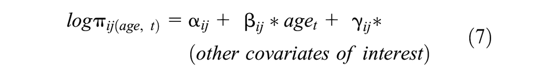
\begin{matrix} \log π_{ij (age, t)} = α_{ij} + β_{ij} * ag e_{t} + γ_{ij} * \\ (other covariates of interest) \end{matrix}

(7)

where, $π_{ij}$ are the instantaneous transition rates to state j $(i, j = 1, 2, \dots \dots, n; i \neq j)$ from the current state i over the annual age interval $ag e_{t}$ .

Application

Data

In our application, we use eight waves of data from the English Longitudinal Survey on Ageing (ELSA). ELSA began following a sample of participants from the 1998 to 2001 Health Survey for England, and now includes eight biennial follow-up waves and five refresher samples. The purpose of ELSA (N = 11,391 core members) is to examine social, psychological, economic, and health changes (and others) among adults ages 50 and older, to better understand and address aging processes and outcomes. The response rate for core members (excluding partners and refreshment samples) ranges from 55% to 82% depending on the wave (for additional information, see Zaninotto & Steptoe, 2019).

In the current study, item missing on work status and occupation, along with missing follow up data on mortality (a combined total of 9% of the full sample at baseline) resulted in an analytic sample of N = 10,332 individuals about whom we had information on work status and other covariates at baseline, and who gave consent to mortality follow up (46.3% women; 53.7% men). Mortality information was followed from the civil registration and linked to ELSA via the National Health Service through 2018.

Measures

Work Status

Work status was measured using information in response to the question: “Which one of these would you say best describes your current situation?” Response categories included, (1) “retired,” (2) “employed,” (3) “self-employed,” (4) “unemployed,” (5) “permanently sick or disabled,” (6) “looking after home or family,” or (7) “other.” Individuals were coded as “in work” if they were “employed” or “self-employed,” thus categories 2 and 3 were collapsed. Individuals were coded as “not in work” if they responded in any other way, and thus, categories 1, 4, 5, 6, and 7 were collapsed.

Covariates

The covariates included in the analysis were sex and occupation. We also stratified the models by these characteristics as prior research continues to show that men and those with higher versus lower occupational levels have longer WLEs (Leinonen et al., 2018; Loichinger & Weber, 2016; Schram et al., 2021). Occupation was measured in terms of occupational level, which included three categories, “professional,”“intermediate,” or “routine,” derived from the National Statistics Socio-Economic Classification (NS-SEC). Professional positions consist of lower management and higher-level positions (e.g., scientist and supervisor); intermediate positions fall between lower management and lower supervisory (e.g., administrative, nonroutine sales and service); and, routine positions include workers from lower supervisory to routine positions (e.g., routine sales, agricultural, child care). Sex was measured in terms of “female” or “male.”

Multistate Analysis for Working Life Expectancy

It is possible that the data indicate observed transitions between non-absorbing states (e.g., working, not working) in a multistate model. Theoretically, there should always be an underlying process of the behavior in a study that determines or informs the multistate model that is adopted. Put another way, the behavior in this application is the stochastic process of changes in work status, which is random; the model adopted represents that unseen process. We assume that all paths are possible among non-absorbing states. The underlying multistate model is the three-state model shown in Figure 1. An individual can be in one of the following state spaces: state (1) “in work” if the individual is working at the time of survey; state (2) “not in work” if the individual is not working at the time of survey; and state (3) “dead” if the individual is deceased. Arrows between each of the states indicate the directions in which instantaneous transitions are allowed.

Figure 1.

Underlying three-state multistate model to estimate working life expectancy.

The primary objective of the current study is to compare WLE estimates between three different statistical packages (see Appendix A for syntax). To do this, we use data from ELSA to estimate WLE by sex and occupation in each of the three packages. Transition probabilities are estimated over the 2-year intervals. In multistate models, the transition times may not always occur at the observed time points in the data. Rather, transition times may occur anytime in between two intervals; this is known as “interval censoring.” Interval censoring is available in the ELECT package, and is thus used in ELECT to estimate WLE. Generally, one’s state space just prior to death is not known. Therefore, if a participant is alive until the end of the observation time and his/her assessment date is not available at that time; we can only say the individual is in either state 1 or state 2. ELECT takes into account this limitation in its calculation of the likelihood of one state space over another (Sutradhar et al., 2011). As recommended (van den Hout et al., 2019), we allow ELECT to work on shifted age, that is, age—50, in order to prevent numerical issues during maximization of the likelihood function.

IMaCh, on the other hand, has the flexibility to estimate transitions over much shorter time intervals, for example, 1 month. SPACE allows for unequal intervals and converts observations into annual intervals to calculate transition probabilities. Given the 2-year gaps in ELSA, SPACE creates pseudo interview data for unobserved years. Events are assumed to occur randomly at one of the annual intervals where there are differences between state spaces over two successive time points. The model assumes only one transition between two time points.

Results

The first wave of the ELSA sample included N = 10,332 individuals ages 50+ and 57,282 person-year observations. Table 1 shows the frequency distribution of the pairs of successive, observed states. There were 215 deaths among those who were “in work” and 3,582 deaths among those who were “not in work.” Moreover, there were few transitions from the state of “not in work” to the state of “in work,” approximately 607 occasions. These were observed frequencies and do not necessarily reflect the transitions in the underlying process of working statuses.

Table 1.

Distribution of Observed Pairs of Consecutive States Among Individuals in ELSA, 2002 to 2018.

State at current time	State at next time (2 years interval)
State at current time	Censored state*	In work	Not in work	Dead
In work	863	7,461	2,622	215
Not in work	1,979	607	29,616	3,587

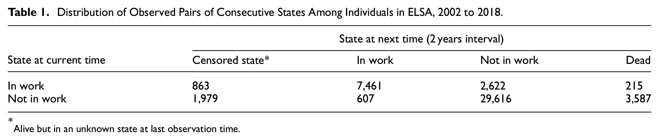
Alive but in an unknown state at last observation time.

The estimates of working life expectancies (WLE) at age 50, along with the 95% confidence intervals for three statistical packages, are presented in Table 2 (for total life expectancies, see Appendix B). The results showed a similar pattern of the estimates by sex and occupation. The pattern was also the same among those ages 50 to 75 years (see Figure 2). Men’s WLE was higher than women’s across all categories of occupation. For example, from the ELECT estimates, professional men age 50 are expected to work an average of 10.5 additional years. The corresponding estimate for women is 8.6 years. The only discernible difference in the stratified analyses (shown in Table 2) was for IMaCh compared to ELECT and SPACE. WLEs were similar across ELECT and SPACE, but were approximately 1 to 2 years different from IMaCh .

Table 2.

Estimates of Working Life Expectancies (WLE) at Age 50 Years by Occupations and Sex.

Sex	Occupations	Working life expectancies [95% CI]
Sex	Occupations	ELECT	IMaCh	SPACE
Men	Professional	10.53 [10.10, 10.99]	11.50 [11.05, 11.95]	10.01 [9.63, 10.44]
	Intermediate	11.44 [10.87, 11.90]	11.83 [11.21, 12.45]	11.02 [10.38, 11.58]
	Routine	9.51 [9.06, 9.94]	10.60 [10.12, 11.07]	9.24 [8.76, 9.54]
Women	Professional	8.62 [8.14, 8.98]	8.90 [8.44, 9.36]	8.43 [7.96, 8.75]
	Intermediate	9.55 [9.04, 9.99]	10.53 [10.02, 11.04]	9.16 [8.77, 9.72]
	Routine	7.66 [7.30, 8.00]	8.09 [7.69, 8.49]	7.69 [7.35, 8.06]

Figure 2.

Total and working life expectancies at single years of age classified by sex and occupational groups.

Discussion

In this study, we took advantage of the longitudinal design and availability of ELSA data from England to compare WLE estimates from three currently available software packages: ELECT in R, the independent package IMaCh, and SPACE in SAS. We extend previous studies (e.g., Cai et al., 2010) on comparisons of software packages used to estimate healthy life expectancy by drawing comparisons between WLE estimates in ELECT, IMaCh, and SPACE. In addition, we estimate WLEs stratified by both sex and occupation. Substantively, we find that WLE patterns were the same across the three statistical packages.

WLE estimates from ELECT, SPACE, and IMaCh are consistent with prior research suggesting significant differences in WLE by occupational status (Leinonen et al., 2018; Schram et al., 2021) and sex (Loichinger & Weber, 2016). For example, Leinonen et al. (2018) find that younger cohorts who worked in manual occupations were expected work 3.5 years fewer than their counterparts in upper non-manual occupations. Although we do not examine younger versus older workers, our findings are consistent in that we find that those in lower skilled, or routine occupations, work approximately 1 to 2 years fewer than those in intermediate and professional occupations. Also consistent with prior research (e.g., Loichinger & Weber, 2016), we find that women’s WLEs are lower than men’s, but WLE patterns are the same across occupations.

Specifically, we find that men’s WLEs at age 50 are highest for those in intermediate occupations (ranging from 11 to 12 years), followed by those in professional occupations (ranging from 10 to 12 years) and lowest for routine workers (ranging from 9 to about 11 years). Women’s WLEs are lower in all occupations (i.e., ranging from 8 years for female routine workers to about 11 years for intermediate and professional workers). Furthermore, for both women and men, we find that WLEs estimates from IMaCh are higher for all occupations compared to those from ELECT and SPACE. One possible explanation for these differences may be that IMaCh does not consider the contribution of deaths to likelihood calculations for those whose dates of death follow the last wave of observation (IMaCh version 0.99r23, March 2021).

IMaCh estimates may also be larger because estimated transition probabilities are slightly higher than those from ELECT and SPACE, as shown in the plots in Appendix B. Transition probabilities from “Not in work” to “In work” (i.e., “2 to 1” in the plot) are slightly higher for men in all occupational categories, thereby slightly increasing the WLE estimates (shown in Table 1). It should also be noted that the msm package, that estimates transition intensities used in the ELECT package, cannot handle survey weights, and may subsequently yield lower WLE estimates. The SPACE package, on the other hand, uses microsimulation to construct life histories for each individual.

Our study further showed that the confidence intervals (CIs) for WLE estimates from IMaCh are narrower than CIs from ELECT and SPACE. This may be due to downwardly biased variance estimates from IMaCh (Cai et al., 2010). SPACE has the capability of correcting the downward bias of variance estimates by using survey weights available in the data. As a result, SPACE has an advantage as one can use complex survey data (Cai et al., 2010). Consistent with our expectations, we found some differences in the estimates from the three statistical packages due to slightly different approaches. Estimates from IMaCh are based on a discrete-time Markov chain and yielded slightly higher WLEs than ELECT and SPACE, which are based on continuous-time Markov chains. Despite slightly different WLEs, the magnitude of the differences is relatively small.

Unlike SPACE and IMaCh, it is possible in ELECT to estimate exact or interval censored transition times. All three packages can handle any number of non-absorbing states; however, the number of states in a given model should be guided by the research question and the available data. In addition, IMaCh is limited in that there should always be a reverse transition for a given transition between two non-absorbing states. Reverse transitions must be possible even when the underlying, theoretical MLST does not suggest a reverse transition between the same two non-absorbing states. This is an important limitation of IMaCh as there are often situations in which reverse transitions are not possible. For example, take a three-state model with health-related state spaces “healthy,”“chronic health condition,” and “death”—it is not possible to transition back to a healthy state space once a person is in a chronic health condition state space, for example, the final stages of terminal cancer.

The MLST approach to estimate working life expectancy provides several advantages over traditional approaches to examining labor force participation and exits. First, WLE estimates give researchers an opportunity to summarize overall average labor force participation in an informative and efficient way. Second, with respect to ELECT, IMaCh, and SPACE, this efficiency is not lost from one package to another with respect to implementation. The computational time to estimate WLEs in each of the three packages is approximately the same. Third, each package uses MSLTs to calculate transition probabilities that are used to estimate WLEs—this may have advantages over, and may be preferable to, previous approaches like the Sullivan method (Mathers, 2000; Nurminen & Nurminen, 2005).

Given that all three approaches utilize transition probabilities or transition intensities from fitting multistate models, it is important to define correctly the multistate model (van den Hout et al., 2019). Moreover, in order to better understand the most appropriate package for a given research problem, future research using simulations that consider different parameters is needed. Overall, however, this study suggests that one could use any of three statistical packages to efficiently estimate WLEs, depending on the ease with which the data can be handled.

The choice of one package over another may depend on whether one has survey or administrative register data, as the latter provides more precise information about the timing of transitions between work statuses. Pedersen and Bjorner (2017), for example, use data from the Danish National Working Environment Survey that are linked to Danish register data of sickness absence and compensation. The latter provides detailed, more precise information on the timing of work statuses (e.g., sickness absences, disability) and allows for estimating WLEs using Cox proportional hazard multistate models (in SAS). This is because information on employment status between survey waves is known. Alternatively, it is possible in ELECT to use either the precise timing or interval timing of transitions between states. Interval censoring is an available option in ELECT, whereas SPACE assumes only one transition between survey waves. It is also important to note that prior research suggests that WLE estimates may be misleading if the precise timing of transitions is incorrectly assumed (Sutradhar et al., 2011). Consideration of these differences may help inform decisions to use one package over another.

Willekens and Putter (2014) note that the advancement of computer programming, combined with the increasing availability of longitudinal data, affords researchers greater opportunities to apply MLST models. As researchers continue to take advantage of these opportunities, we stand to contribute significantly to better understanding who can and will work later in life. By extension, such research could help to inform ongoing policy discussions about the old-age dependency ratio, including whether or not governments should extend the working life.

Footnotes

Appendix

Appendix B.

Total Life Expectancies (TLE) at Age 50 Years by Occupation and Sex.

Sex	Occupation	Total life expectancies [95% CI]
Sex	Occupation	ELECT	IMaCh	SPACE
Men	Professional	30.86 [30.11, 31.50]	31.89 [31.28, 32.50]	32.38 [31.65, 32.94]
	Intermediate	29.38 [28.40, 30.06]	30.48 [29.74, 31.22]	31.19 [30.43, 31.85]
	Routine	27.79 [27.22, 28.28]	28.75 [28.21, 29.29]	28.78 [28.13, 29.43]
Women	Professional	34.42 [33.63, 35.10]	35.29 [34.58, 35.99]	35.24 [34.64, 35.85]
	Intermediate	32.85 [32.03, 33.55]	33.71 [33.00, 34.41]	33.77 [33.19, 34.46]
	Routine	31.15 [30.55, 31.70]	31.93 [31.40, 32.47]	31.51 [30.83, 32.20]

Acknowledgements

The authors would like to thank participants of the 32nd meeting of the REVES Network of Health Expectancy for helpful comments on an earlier version of this work.

Declaration of Conflicting Interests

The author(s) declared no potential conflicts of interest with respect to the research, authorship, and/or publication of this article.

Funding

The author(s) disclosed receipt of the following financial support for the research, authorship, and/or publication of this article: This study was funded by the Swedish Research Council for Health, Working Life and Welfare (Forte, grant #2019-01321). Chungkham and Högnäs contributed equally as first authors to the manuscript. Please direct all correspondence to Holendro Singh Chungkham, holendro.chungkham@su.se or Robin S. Högnäs, robin.hognas@su.se, both at the Stress Research Institute, Stockholm University, Sweden.

ORCID iDs

Holendro Singh Chungkham

Robin S. Högnäs

References

Barendregt

J. J.

Bonneux

van der Maas

P. J.

(1997). How good is Sullivan’s method for monitoring changes in population health expectancies? Journal of Epidemiology and Community Health, 51(5), 578–579. https://doi.org/10.1136/jech.51.5.578

Cai

Hayward

M. D.

Saito

Lubitz

Hagedorn

Crimmins

(2010). Estimation of multi-state life table functions and their variability from complex survey data using the SPACE program. Demographic Research, 22, 129–158. https://doi.org/10.4054/DemRes.2010.22.6

Crimmins

E. M.

Hayward

M. D.

Saito

(1994). Changing mortality and morbidity rates and the health status and life expectancy of the older population. Demography, 31(1), 159–175. https://doi.org/10.2307/2061913

Department for Work and Pensions. (2017). Fuller working lives: A partnership approach. https://www.gov.uk/government/uploads/system/uploads/attachment_data/file/587654/fuller-working-lives-a-partnership-approach.pdf

Doyle

McKee

Rechel

Grundy

(2009). Meeting the challenge of population ageing. BMJ (Online), 339(7726), 892–894. https://doi.org/10.1136/bmj.b3926

Dudel

López Gómez

M. A.

Benavides

F. G.

Myrskylä

(2018). The length of working life in Spain: Levels, recent trends, and the impact of the financial crisis. European Journal of Population, 34(5), 769–791. https://doi.org/10.1007/s10680-017-9458-9

Foster

E. M.

Skoog

G. R.

(2004). The markov assumption for worklife expectancy. Journal of Forensic Economics, 17(2), 167–183. https://doi.org/10.4135/9781412983907.n469

Giandrea

M. D.

Cahill

K. E.

Quinn

J. F.

(2009). Bridge jobs: A comparison across cohorts. Research on Aging, 31(5), 549–576. https://doi.org/10.1177/0164027509337195

Hanson

L. L. M.

Westerlund

Chungkham

H. S.

Vahtera

Rod

N. H.

Alexanderson

Goldberg

Kivimäki

Stenholm

Platts

L. G.

Zins

Head

(2018). Job strain and loss of healthy life years between ages 50 and 75 by sex and occupational position: Analyses of 64 934 individuals from four prospective cohort studies. Occupational and Environmental Medicine, 75(7), 486–493. https://doi.org/10.1136/oemed-2017-104644

10.

Hayward

M. D.

Grady

W. R.

(1990). Work and retirement among a cohort of older men in the United States 1966–1983. Demography, 27(3), 337–356. https://doi.org/10.2307/2061372

11.

Head

Hyde

(2020). Measuring progress toward healthy working lives. Lancet Public Health, 5(7), e366–e367. https://doi.org/10.1016/j.athoracsur.2020.04.003

12.

Jackson

C. H.

(2011). Multi-state models for panel data: The msm package for R. Journal of Statistical Software, 38(8), 1–28. https://doi.org/10.18637/jss.v038.i08

13.

Laditka

S. B.

Wolf

D. A.

(1998). New methods for analyzing active life expectancy. Journal of Aging and Health, 10(2), 214–241. https://doi.org/10.1177/089826439801000206

14.

Leinonen

Martikainen

Myrskylä

(2018). Working life and retirement expectancies at age 50 by socioeconomic status: Period and cohort trends and projections for Finland. Journals of Gerontology – Series B Psychological Sciences and Social Sciences, 73(2), 302–313. https://doi.org/10.1093/geronb/gbv104

15.

Lièvre

Brouard

Heathcote

(2003). The estimation of health expectancies from cross-longitudinal surveys. Mathematical Population Studies, 10(4), 211–248. https://doi.org/10.1080/713644739

16.

Loichinger

Weber

(2016). Trends in working life expectancy in Europe. Journal of Aging and Health, 28(7), 1194–1213. https://doi.org/10.1177/0898264316656509

17.

Mathers

C. D.

(2000). Health expectancies – an overview and critical appraisal. In Murray

Salomon

Mathers

Lopez

(Eds.), Summary measures of population health: Concepts, ethics, measurement and applications (pp. 177–204). World Health Organization.

18.

Mathers

C. D.

Robine

J. M.

(1997). How good is Sullivan’s method for monitoring changes in population health expectancies. Journal of Epidemiology and Community Health, 51(1), 80–86. https://doi.org/10.1136/jech.51.1.80

19.

Nurminen

Heathcote

Davis

(2004). Estimating marginal cohort working life expectancies from sequential cross-sectional survey data. Journal of Official Statistics, 20(3), 495–515.

20.

Nurminen

(2005). Multistate worklife expectancies. Scandinavian Journal of Work, Environment and Health, 31(3), 169–178. https://doi.org/10.5271/sjweh.866

21.

OECD. (2019). Society at a glance: OECD social indicators (pp. 1–131). OECD Publishers.

22.

Ophir

(2022). The paid and unpaid working life expectancy at 50 in Europe. Journals of Gerontology: Social Sciences, 77(4), 769–779.

23.

Pedersen

Bjorner

J. B.

(2017). Worklife expectancy in a cohort of Danish employees aged 55–65 years – comparing a multi-state Cox proportional hazard approach with conventional multi-state life tables. BMC Public Health, 17(1), 1–11. https://doi.org/10.1186/s12889-017-4890-7

24.

Pedersen

Schultz

B. B.

Madsen

I. E. H.

Solovieva

Andersen

L. L.

(2020). High physical work demands and working life expectancy in Denmark. Occupational and Environmental Medicine, 77, 576–582.

25.

Platts

L. G.

Corna

L. M.

Worts

McDonough

Price

Glaser

(2019). Returns to work after retirement: A prospective study of unretirement in the United Kingdom. Ageing and Society, 39(3), 439–464. https://doi.org/10.1017/S0144686X17000885

26.

Reynolds

S. L.

McIlvane

J. M.

(2009). The impact of obesity and arthritis on active life expectancy in older Americans. The Gerontologist, 45(4), 438–444. https://doi.org/10.1038/oby.2008.534

27.

Rueda-Salazar

Spijker

Devolder

Albala

(2021). The contribution of social participation to differences in life expectancy and healthy years among the older population: A comparison between Chile, Costa Rica and Spain. PLoS One, 16(3), 1–24. https://doi.org/10.1371/journal.pone.0248179

28.

Schram

J. L. D.

Solovieva

Leinonen

Viikari-Juntura

Burdorf

Robroek

S. J. W.

(2021). The influence of occupational class and physical workload on working life expectancy among older employees. Scandinavian Journal of Work, Environment and Health, 47(1), 5–14. https://doi.org/10.5271/sjweh.3919

29.

Sullivan

D. F.

(1971). A single index of mortality and morbidity. HSMHA Health Reports, 86(4), 347–354. https://doi.org/10.2307/4594169

30.

Sutradhar

Barbera

Seow

Howell

Husain

Dudgeon

(2011). Multistate analysis of interval-censored longitudinal data: Application to a cohort study on performance status among patients diagnosed with cancer. American Journal of Epidemiology, 173(4), 468–475. https://doi.org/10.1093/aje/kwq384

31.

van den Hout

Sum Chan

Matthews

(2019). Estimation of life expectancies using continuous-time multi-state models. Computer Methods and Programs in Biomedicine, 178, 11–18. https://doi.org/10.1016/j.cmpb.2019.06.004

32.

Weber

Loichinger

(2020). Live longer, retire later? Developments of healthy life expectancies and working life expectancies between age 50–59 and 60–69. European Journal of Ageing, 19, 75–93. https://doi.org/10.1007/s10433-020-00592

33.

Willekens

Putter

(2014). Software for multistate analysis. Demographic Research, 31(1), 381–420. https://doi.org/10.4054/DemRes.2014.31.14

34.

Zaninotto

Steptoe

(2019). English longitudinal study of ageing. In Gu

Dupre

(Eds.), Encyclopedia of gerontology and population aging (pp. 1–7). Springer.

Estimating Working Life Expectancy: A Comparison of Multistate Models

Abstract

Keywords

Three Multistate Models

Interpolated Markov Chains (IMaCh)

Elect

Space

Application

Data

Measures

Work Status

Covariates

Multistate Analysis for Working Life Expectancy

Results

Discussion

Footnotes

Appendix

Acknowledgements

Declaration of Conflicting Interests

Funding

ORCID iDs

References