Sage Journals: Discover world-class research

Abstract

This paper attempts to investigate if the effect of oil price on growth is asymmetrical for Malaysia, a small-open-dynamic oil-exporting country, over a period from 1981 to 2017. The empirical method employed in this study is the augmented autoregressive distributed lag model (ARDL) bound test approach and the recent innovative nonlinear autoregressive distributed lag (NARDL) model. Results suggest that neglecting nonlinearities can lead to misleading results. More precisely, the result reveals that adjustments in the price of oil influence Malaysia’s economic growth asymmetrically. An increase and decrease in the price of oil strengthen the economic growth of Malaysia, demonstrating Malaysia’s ability to be both an oil-producing country and a trading nation. These results strongly imply that Malaysia is able to take advantage of changes in the oil price efficiently.

Keywords

economic growth oil price shocks oil exporting asymmetric effect Malaysia

Introduction

Crude oil continues to be a key input in production activity, where oil price variations can play an enormous role in most oil-exporting countries economic growth, and Malaysia is no exception. Malaysia, a small-open-dynamic economy, is amongst the very few ASEAN net oil-exporters. Accordingly, the oil industry has been instrumental in structuring the economic progress of Malaysia. They act as an instrumental driving force in the economic development of Malaysia due to its high reliance on oil revenue. Based on the US Energy Information Agency (Eia, 2019) data, Malaysia is a net oil-exporter whose proven crude oil reserves is approximately 3.60 billion barrels, which is 0.22% of the 1,645.74 billion barrels of world proven crude oil reserves and 26.92% of the 13.37 billion barrels of proven crude oil reserves within the ASEAN region, as of 2017. Despite accounting for a small percentage of the total world proven crude oil reserves, Malaysia remains one of the top 25 countries that exported the most petroleum crude oil in the year 2017, as reported by the United Nations Commodity Trade Statistics Database (COMTRADE). This remarkable feat makes Malaysia susceptible to the international oil market.

Moreover, the total trade value of export of petroleum crude oil to Malaysia’s top five importers alone was a whopping 5.92 billion USD in the year 2017. During that same year, the total oil revenue accrued by Malaysia was MYR32.18 billion (roughly 7.5 billion USD), a considerable sum of money. Larger figures can be expected when the crude oil price is higher. The significant role played by the oil sector in providing financial resources for investment activities and therefore contributing to the Malaysian economics development process is depicted in Figure 1.

Figure 1.

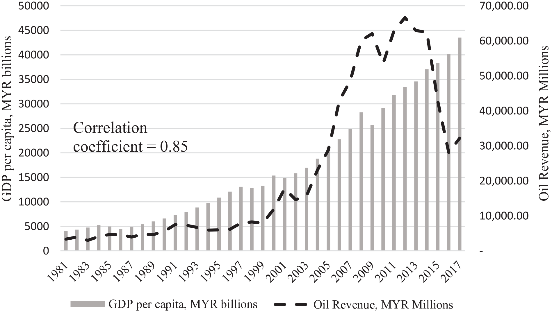
Co-movement between Malaysia’s GDP per capita and oil revenue.

As a matter of fact, any changes and development in the global fluctuations in the prices of oil can substantially affect the structure of Malaysia’s economy. This is shown throughout the co-movement of the Malaysian GDP per capita and oil revenue which is utilized to measure the oil price, as illustrated in Figure 1. Both variables move together, having a strong correlation coefficient of approximately 85%. A case in point, rising oil prices between 2002 and 2008 have raised Malaysia’s oil earnings at an average of MYR40,710 per year compared to MYR 11,399 over the period 1997 to 2002, while real GDP per capita recorded an average of 11.3% in comparison to 2.9% over the same period, reflecting a large volume of revenues per year over the period 2002 to 2008. Conversely, a fall in oil prices throughout 2012 to 2013, have decreased oil revenues to an average of MYR 66,617 million per year, which affected its economic growth at a mere average of just 3.1% throughout the same period.

However, comprehensive studies on net oil exporters remain limited. More often than not, assumptions that rising oil prices supposedly boost the economy of oil-rich nations is inaccurate, as this may not always be the case. In fact, it might even undermine economic growth. Such is the case for certain African countries with low per capita income, despite having vast natural resources, while certain East Asian economies with almost no exportable natural resources could achieve a high living standard (Frankel, 2010). This paradox, known as the “natural resource curse,” is a term coined by Auty (1993). Subsequently, various research has reaffirmed this paradox (Cheng et al., 2020; Naseer et al., 2020; Papyrakis & Gerlagh, 2004). There are multiple theories that provide an explanation for this curse. One of these theories is the worsening of the economic climate that is conducive to economic growth due to the rent-seeking behavior, currency appreciation, and poor policy-making in the wake of an increase in oil revenues (Moshiri & Banihashem, 2012). As such, the higher price of oil could potentially be hurting the economy of oil-exporters instead of strengthening it. This highlights that the outright presumption that oil price and various other macroeconomic variables have a linear relationship between them seems inappropriate as the oil price-macroeconomic nexus could potentially be more complex than a simple linear model. Nusair (2016)’s model, for instance, implies that the effects of oil shocks on the oil exporter’s economic activities may have an asymmetric effect in nature. Nevertheless, empirical findings on oil price-economic growth relationship from an asymmetric approach, especially with regard to developing and emerging economies that act as oil-exporting countries, like Malaysia, seems to be inadequate and scant.

In line with the sizable dependence on oil revenues, an extensive study on the effects of oil price on the Malaysian economy is timely and crucial. Therefore, this study attempts to exclusively examine the asymmetric effect of oil price on the economic growth of Malaysia by employing the Nonlinear Autoregressive Distributed Lag (NARDL) model of Shin et al. (2014) approach, which is the extended version of the Autoregressive Distributed Lag (ARDL) model as established by Pesaran et al. (2001).

Given that empirical studies remain limited, specifically in the ASEAN region, hence this study is deemed relevant in bridging the gap by empirically scrutinizing the effects that variation in the prices of oil has on the economic growth of Malaysia. The purpose of this study extends prior studies in numerous aspects. Firstly, there are limited studies that discern the oil shocks (i.e., positive changes and negative changes) and, thereby, making implicit assumptions that oil prices affect macroeconomic activities symmetrically. An exception to that is a recent study by Bala and Chin (2020), who employed the Nonlinear Autoregressive Distributed Lag Approach (NARDL) model by Shin et al. (2014) and found that oil price increase boosts economic growth while a decrease yields insignificant results. However, a major drawback from this study is the improper conclusion of asymmetric effect, as the Wald-test for long-run and short-run symmetry, which are integral in a NARDL approach, was disregarded. As such, the authors’ conclusion that asymmetry exist is misleading and questionable. Secondly, this study only applies a single F-test for the joint significance of lagged variables alone to determine if cointegration exists, which is insufficient, to say the least. Most existing ARDL and NARDL approaches would at least take into consideration a t-test on the lagged level of the dependent variable, as highlighted by Pesaran et al. (2001).

Therefore, this study leads to endeavor the validity of nonlinear hypothesis on the linkages between oil price shocks and economic growth, for a small-open-dynamic economy, namely Malaysia, through the use of the augmented NARDL model. The use of such a model is suitable for this analysis as it also inherits the advantages obtained from the use of an ARDL model, for instance, the ability to run a regression with mix order of integration of variables. As the variables used in this paper are mixed, such regression techniques become necessary. Furthermore, the augmented NARDL model allows the decomposition of the positive and negative partial sum of the selected explanatory variable (i.e., oil revenue), which would provide a revelation on how variation in oil prices affects the economic growth of Malaysia asymmetrically. An augmented ARDL and NARDL model is also more stringent than the ordinary ARDL and NARDL model, whereby three statistical tests, that is, F-statistic for lagged level variables, t-statistic for lagged dependent variable and F-statistic for lagged independent variables, are needed to conclude whether a cointegrating relationship exists.

Secondly, this paper employs oil revenue as computed based on the total petroleum income tax, petroleum royalty and PETRONAS dividend, as opposed to the typical proxy in most literature, oil price. This utilization of an unconventional proxy stems from the idea that an adjustment in oil exports could be utilized as a way to mitigate the effects of oil price on the economy (Moshiri & Banihashem, 2012). Such adjustment might transpire, mainly when the price of oil is low, prompting the government to increase oil exports to stabilize the oil revenue. This adjustment then results in an increment in the oil revenue following the higher oil exports, which may substantially benefit the economy should the prices of oil be low. Put differently; an oil-exporter can nullify the negative effect that is often associated with low oil prices. In such cases, the utilization of oil prices in determining the economic performance of an oil-exporter seems to be immaterial and potentially flawed. On the other hand, oil revenues are capable in providing a better picture on the linkages between crude oil price-economic growth while avoiding biases stemming from oil exports, making it a superior measurement than the oil price. To the best of our knowledge, this concept has only been implemented in a handful of previous studies (Abdlaziz et al., 2021, 2022; Charfeddine & Barkat, 2020; Olayungbo, 2019) and remains an intriguing aspect worth exploring when dealing with oil-price related studies.

Thirdly, previous studies that merely pay attention to the bivariate relationship between prices of oil and growth could potentially be misspecified, leading to biased results, when certain relevant explanatory variables are excluded (Bouoiyour et al., 2015). This highlights the significance of considering potential control variables to reach more precise and conclusive results. Hence, this paper takes into account the interdependence between the price of oil and economic growth by incorporating additional control variables (i.e., human capital, investment and population) that could potentially elucidate the oil price-growth nexus more effectively.

The remainder of this study is structured as follows: Section 2, exhaustively reviews the relevant literature to this study on oil price-economic growth. Section 3 explains the model specification, econometric formulation and cointegration analysis. Section 4 discusses the empirical results obtained from the econometric analysis. Section 5 concludes with the findings and policy implications.

Background and Literature Review

Research on the macroeconomic effects of oil price has been profound. An influential work of Hamilton (1983), discovered that post World War II oil price increases played a part in every US recession that occurred after that. Overall, the consensus among early studies is that the oil price-economic growth relationship is inverse. Such studies, however, emphasizes on oil-importing countries.

Indeed, Mork (1989) has paved a new dimension on the oil price-economic growth nexus by introducing asymmetric effects in oil price. In his study, several producer price indices are utilized to proxy for crude oil price and through the segregation of increase and decrease in the prices of oil, allowed the asymmetric feedback from the US economic activity in response to changes in real oil prices to be captured. Through the segregation, it is ascertained that a positive change in oil price has a substantially significant negative relationship with real GNP changes. However, a decrease in oil price was not significant. The differences between the increase and decrease in the interest variable, strongly imply that the asymmetric effect exists, thus invalidating the linear effect. This revelation has been a stepping stone in proliferating future studies on the nonlinear effects within the oil price-macroeconomic nexus using different techniques such as GARCH model and multivariate VAR analysis (Elder & Serletis, 2010; Hamilton, 1996; Jiménez-Rodríguez & Sánchez, 2005; Lee et al., 1995).

In addition, some studies have also directed the research interest from oil importers and developed economies toward the effect of changes in the prices of oil on the macroeconomics of developing nations. Notably, the primary concern of this study is to center the discussion on the net oil-exporters. For instance, Jiménez-Rodríguez and Sánchez (2005) conclude on the differential effect between oil importers and oil exporters, through the multivariate VAR analysis. They discovered that rising oil prices are detrimental toward the economic activity of oil importers, whereas the effect on oil exporters was deemed uncertain. In the case of Kuwait, Eltony and Al-Awadi (2001) studied the effects of oil price shocks on the macroeconomic variables. They discovered that the symmetric oil price shocks played an influential role in interpreting the fluctuation on macroeconomic variables, specifically a critical factor in influencing the level of economic progress for Kuwait seems to be shocks of oil price. Thereafter, Berument et al. (2010) who investigated the economic impacts of oil price shocks on a group of Middle Eastern and North African countries found conflicting results. Results from the study suggest that the prices of oil exert a positive growth effect for Algeria, Iraq, Jordan, Kuwait, Oman, Qatar, Syria, Tunisia and UAE, whereas the other countries like Bahrain, Egypt, Lebanon, Morocco and Yemen have found no such evidence. Furthermore, Olomola and Adejumo (2006) also discovered that shocks in oil prices do not have any profound effects on the output for the case of Nigeria. They conclude that this may be explained through the phenomena of Dutch disease in which the tradable sector has been squeezed as a result of exchange rate appreciation.

These mixed findings have switched the discussion to the nonlinear perspective. One of the earliest studies that unraveled the nonlinear effect of oil price on growth theory was the Dutch disease theory established by Corden and Neary (1982). In oil-exporting nations, a shift in the economic structure from manufacturing and agriculture toward oil and non-traded sectors takes place when oil prices are high. Moreover, the rise in oil revenues will also result in an appreciation of the domestic currency, resulting in higher imports of intermediate and consumer goods. The growing dependence on foreign goods then harms the local industries who are incapable of competing when oil prices are high. From a Dutch disease perspective, temporary exchange rate appreciations do more harm than good for the economy. Lower oil prices have opposing outcomes. However, several empirical studies are unable to substantiate this theory. Ito (2017), for instance, concluded that Russia is unaffected by Dutch disease. From an exchange rate perspective, Korhonen and Mehrotra (2009) discovered that oil shocks failed to capture a significant portion of the real exchange rate movements.

In recent literature, the theory on the asymmetric effect, which has been emphasized by Mork (1989) appears to be used to portray further the explanation of the oil price-growth nexus among oil-exporters. For example, Moshiri and Banihashem (2012) studied whether the oil price movements in the economy of the six OPEC countries have an asymmetric effect. Accordingly, during higher oil price period accompanied by higher revenues, governments tend to spend aggressively on projects with unsustainable economic growth. However, during the lower oil price phase leading to significant revenue cuts, large investment projects remain incomplete, and thus, most economic activities are halted. Poor management, rent-seeking behavior and inadequate transparency and competition are factors that repress the country from fully benefiting from the higher oil price while being entirely susceptible to lower oil price. This finding implies the presence of an asymmetric effect of oil price shocks on growth.

This conjecture of asymmetric effect of oil price shocks on economic growth is further supported by Farzanegan and Markwardt (2009), Kose and Baimaganbetov (2015), and Donayre and Wilmot (2016) who discovered that the shocks in oil prices have an asymmetric effect on the economic activities of oil-exporting nations. A recent paper by Nusair (2016), using the nonlinear autoregressive distributed lag (NARDL) model of Shin et al. (2014), further confirmed this finding. Specifically, this study found that in all cases, positive changes in the prices of oil have a significant positive sign, implying that an expansion in the real GDP is expected following an increase in the prices of oil. On the other hand, adverse changes in the prices of oil have a significant positive sign only for Kuwait and Qatar, which indicate that a decrease in the prices of oil will be detrimental for the GDP of these countries. The results also emphasize on the relevance of asymmetric effect in the growth-enhancing strategy of oil price shocks. Another study conducted by Charfeddine and Barkat (2020) on Qatar, also found a strong evidence of asymmetric effect in the real oil prices and real oil and gas revenues on the total real GDP and non-oil real GDP.

In the case of Malaysia, Aziz and Dahalan (2015) investigated the effect of oil price on the economic performance of five countries, including Malaysia, by employing a panel VAR model. This study used Mork’s (1989) model to distinguish the effect between positive changes and negative changes in oil price. Results suggest that the asymmetric effect exists for the selected countries. However, the results of this study also discovered that GDP responses negatively toward the oil price. This finding nonetheless seems to be hardly surprising given the fact that a panel data approach was employed, which could potentially suffer from heterogeneity issues since the response of the all the underlying countries toward movements in the price of oil will not be the same. Another notable study that includes Malaysia was conducted by Kriskkumar and Naseem (2019). Using the Augmented ARDL model and NARDL model, they found that the effect of oil price on economic growth was insignificant in the long-run for both the linear and nonlinear models. Similarly, a study conducted by Khan et al. (2019) also found that no long-run asymmetry in the oil price-economic activity nexus using the NARDL model, for the case of Malaysia. An issue that may arise from such studies is the use of oil price instead of oil revenue, whereby adjustments in the oil revenue through higher oil exports may nullify the negative effect that is often associated with low oil prices.

In short, research on the oil price-economic growth linkage concerning the asymmetric effect is still in its infancy. More importantly, in the case of a small-open-dynamic oil-exporting country like Malaysia, there is still no definite conclusion on the presence of the asymmetric effect. Therefore, the evidence from past studies has led to an in-depth study on the effect of oil price on economic growth, under a nonlinear framework.

Methodology

Model Specification

In favor of this study, the effect of oil price on economic growth can be derived based on the following three-factor Cobb-Douglas production function:

Y_{t} = K_{t}^{α} H_{t}^{β} {(A_{t} L_{t})}^{1 - α - β}

(1)

whereby Y is the aggregate income, K is the physical capital, H is the human capital, A is the labor augmenting factor representing the efficiency level of each worker, L is the size of the labor force and the subscript t denotes time. α and β represent the respective proportion of each production factor with the assumption of constant return to factors. In the Cobb-Douglas model, a constant return of scale is implied when $α + β = 1$ . However, due to the assumption of diminishing returns of capital, the condition is set to $α + β < 1$ . Size of labor, L and labor augmenting factor, A are assumed to grow at an exogenous growth rate of n and g, respectively, such that:

L_{t} = L_{0} e^{n t}

(2)

A_{t} = A_{0} e^{g t + P θ}

(3)

whereby n is the growth rate of the labor size, g is the growth rate of efficiency level, P is oil revenue which can promote economic growth, and θ is the coefficient for P. Moreover, output per worker increases at a constant rate of g, under the steady-state. Such outcome is obtainable through the definition of output per worker such that:

\frac{Y_{t}}{L_{t}} = A_{t} k_{t}^{α} h_{t}^{β}

(4)

where k is the physical capital per population and h is the human capital per population. Taking logs of both sides of equation (4) at time 0 for simplicity, we get the following:

L n \frac{Y}{L} = L n A + α L n k + β L n h

(5)

given $A_{t} = A_{0} e^{g t + P θ}$ ,

\begin{array}{l} L n \frac{Y}{L} = L n A_{0} + g t + P θ + \frac{α}{1 - α - β} L n S_{K} \\ + \frac{β}{1 - α - β} L n S_{H} - \frac{α + β}{1 - α - β} L n (n + g + δ) \end{array}

(6)

Equation (6) shows the steady-state for output per worker. P is the oil revenue variable, δ is the depreciation rate, while $\frac{α}{1 - α - β}$ , $\frac{β}{1 - α - β}$ , and $\frac{α + β}{1 - α - β}$ are the elasticities for the saving rate of physical capital, the saving rate of human capital and labor growth per capita income, respectively. Due to data limitation, $g t$ is assumed to be time-invariant while $S_{K}$ , $S_{H}$ and n can vary over time. In other words, we can consider $A_{0}$ and $g t$ to be constant term, $A_{0}$ in equation (7). Hence, the equation will now be:

\begin{array}{l} L n \frac{Y}{L} = A_{0} + P θ + \frac{β}{1 - α - β} L n S_{H} \\ - \frac{α + β}{1 - α - β} L n (n + g + δ) + \frac{α}{1 - α - β} L n S_{K} \end{array}

(7)

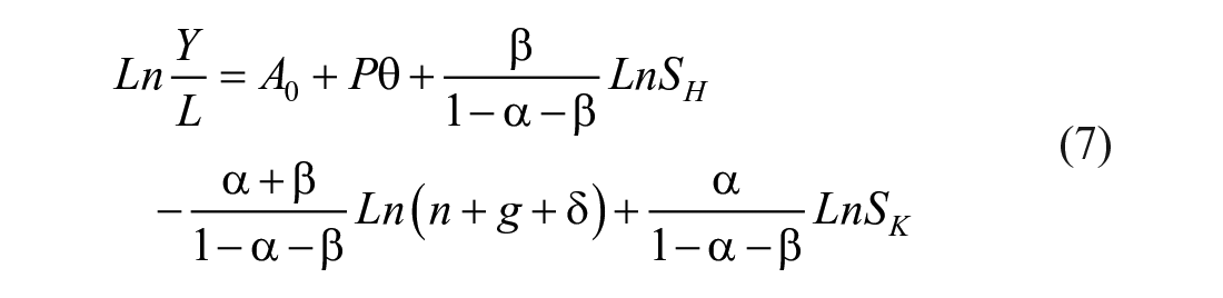
By rearranging equation (7), we can then reduce the equation to the following:

\begin{array}{l} L n R G D P P C_{t} = a + b L n O I L_{t} + c L n H C_{t} \\ + d L n P O P G_{t} + e L n G F C F_{t} + ε_{t} \end{array}

(8)

where RGDPPC denotes the real gross domestic product per capita, OIL refers to the real oil revenue, which is utilized as a proxy for the price of oil, HC is the human capital index, POPG signifies population growth, GFCF indicates gross fixed capital formation as a measure of investment and $ε_{t}$ is the white-noise disturbance term. The multivariate specification in equation (8) is as established by Levine and Renelt (1992), Campos (2001), Azman-Saini et al. (2010), and Kriskkumar and Naseem (2019), with the additional inclusion of the oil revenue variable.

The sensitivity of the variables in this growth model is expressed via the parameters, b, c, d, and e of the model, which are widely identified in the literature of economic growth. The estimate for b is expected to have a positive sign. An increase in oil revenue is often beneficial in the case of an oil-exporter like Malaysia because a portion of the government coffers comprises of oil revenue. Hence, a higher price of oil translates to rising oil revenue. With that, the government can finance its expenditures as well as invest in the development of the country and in doing so, promote economic growth. Human capital is often deemed as a fundamental aspect of the economy (Mankiw et al., 1992; Qadri & Waheed, 2014; Romer, 1986). Adequate education, skills and good health are crucial elements in creating a productive workforce that will enhance national economic growth (Bloom et al., 2004). Hence, the coefficient estimate of c is expected to be positive.

Additionally, labor growth is another key determinant of growth (Frankel, 1962), which is proxied by population growth in this study. An increase in population growth reflects a diminishing capital to labor ratio since the capital must be allocated more thinly among the broader workforce, hence adversely affecting GDP per capita (Mankiw et al., 1992). On the other hand, the capital stock, a fundamental factor within the production function, is proxied by GFCF. Increase in the capital stock improves multifactor productivity, resulting in greater productivity and efficiency (Sharma, 2010). Therefore, the expected coefficient estimate of GFCF is positive.

Econometric Methodology

Augmented Autoregressive Distributed Lag (ARDL) Model

This study employs the McNown et al.’s (2018) Augmented Autoregressive Distributed Lagged (ARDL) bounds test for cointegration. This approach is an extension of the ARDL bounds test approach by Pesaran et al. (2001). In theory, this approach can be employed to determine if the underlying variables have a long-run relationship even though the order of integration of the variables are different, unlike conventional cointegration tests (i.e., Johansen & Juselius, 1990). This proposes one of the key benefits of the ARDL model, where the variables are allowed to be integrated of order zero, one or fractionally integrated. In addition, cointegration analysis involving small sample sizes are robust using the bounds testing approach (Pesaran et al., 2001). Mah (2000), for instance, mentioned that conventional tests for cointegration, like the Engle and Granger (1987) or Johansen and Juselius (1990), have a propensity for unreliability in small sample sizes. Based on the bounds testing procedure, equation (8) must primarily be modeled as a conditional ARDL with the following specifications:

\begin{array}{l} Δ L n R G D P P C_{t} = λ_{0} + λ_{1} L n R G D P P C_{t - 1} \\ + λ_{2} L n O I L_{t - 1} + λ_{3} L n H C_{t - 1} \\ + λ_{4} L n P O P G_{t - 1} + λ_{5} L n G F C F_{t - 1} \\ + \sum_{k = 1}^{n} β_{k} Δ L n R G D P P C_{t - k} + \sum_{k = 0}^{n} δ_{k} Δ L n O I L_{t - k} \\ + \sum_{k = 0}^{n} φ_{k} Δ L n H C_{t - k} + \sum_{k = 0}^{n} \partial_{k} Δ L n P O P G_{t - k} \\ + \sum_{k = 0}^{n} π_{k} Δ L n G F C F_{t - k} + ε_{t} \end{array}

(9)

where ∆ is the first difference operator and $ε_{t}$ is a white-noise disturbance error term. The equation above can provide the short-run and long-run estimates within a single-equation framework. The estimates for the short-run effects are obtainable from the coefficient of the respective first differenced while the estimates for the long-run effects are obtainable from equation (9) by normalizing the coefficients of $λ_{2}$ to $λ_{5}$ on $λ_{1}$ . Nevertheless, estimates for the long-run are only meaningful provided that cointegration can be established. Hence, to establish the presence of cointegration, three separate tests need to be applied.

The first test is the F-test for the joint significance of lagged variables, as recommended by Pesaran et al. (2001). This test is also known as a bounds test. If the calculated F-statistic is below the lower bound value, the null hypothesis of no long-run relationship cannot be rejected whereas if the calculated F-statistic is greater than the upper bound value, the null hypothesis can be rejected, signifying the presence of a cointegrating relationship. Nevertheless, if the calculated F-statistic falls between the lower and upper bound value, the result is inconclusive. Given that the sample size for this research is less than 80, the lower bound and upper bound critical values provided by Narayan (2005) will be used instead.

The second test is the t-test on the lagged level of the dependent variable, which is also suggested by Pesaran et al. (2001). In the bounds test approach, Pesaran et al. (2001) suggested running a t-test to eliminate the possibility of degenerate lagged dependent variable case. Such test is necessary because the significance of the F-test for joint significance of lagged variables may stem purely from the lagged independent variable(s) or the lagged level of the dependent variable alone. For this particular test, the critical value provided by Pesaran et al. (2001) on pp. 303–304 will be used. Similar to the F-test for the joint significance of lagged variables, this study can establish statistical significance if the calculated t-statistic values exceed the upper bound critical value.

The third test is an additional test introduced by McNown et al. (2018), which is an F-test on the lagged levels of the independent variable(s). This test will avoid the assumption that the dependent variable is I(1), which was made by Pesaran et al. (2001), to rule out degenerate lagged independent variable(s) case. However, given the lower power from standard unit root tests, the additional F-test proposed by McNown et al. (2018) will resolve this issue. Similar to the bounds test proposed by Pesaran et al. (2001), the F-statistic computed from this test will be referred to the critical values provided by Sam et al. (2019). If the F-statistic exceeds the upper bound, the null hypothesis is rejected, and the test is significant while an F-statistic below the lower bound, the null hypothesis is accepted, and the test is insignificant. In the case where the F-statistic falls between the lower bound and the upper bound, the test is inconclusive. All the three-tests suggested will present a more accurate conclusion on the cointegration status of the model.

From the three cointegration tests proposed above, there are a total of four possible outcomes depending on the results obtained. The first outcome is a degenerate lagged dependent variable case, also referred to as degenerate case #1 (see Goh et al., 2017; McNown et al., 2018). In degenerate case #1, out of the three cointegration test proposed above, the t-test on the lagged dependent variable turns out to be insignificant. The second outcome is a degenerate lagged independent variable, also referred to as degenerate case #2. In degenerate case #2, both the traditional the F-test for the joint significance of lagged variables and the t-test on the lagged dependent variable is significant except the newly proposed F-test on the lagged independent variable(s). The third outcome is when the F-test for the joint significance of lagged variables is insignificant. In this case, it is not necessary to perform the t-test on the lagged dependent variable and the F-test on the lagged independent variable(s). In the fourth outcome, all three cointegration tests are significant. Only the fourth outcome implies cointegration among the cointegrating variables.

Nonlinear Autoregressive Distributed Lag (NARDL) Model

As previously mentioned, the effect of oil price on economic growth could be asymmetric. Hence, the NARDL model developed by Shin et al. (2014), which is an extension of the Pesaran et al. (2001) linear ARDL bound testing approach is employed. This methodology allows the decomposition of the independent variables such as oil price into both positive and negative partial sum of processes

\begin{matrix} P O S = \sum_{j = 1}^{t} Δ L n O I L_{j}^{+} = \sum_{j = 1}^{t} \max (Δ L n O I L_{j}, 0), \\ N E G = \sum_{j = 1}^{t} Δ L n O I L_{j}^{-} = \sum_{j = 1}^{t} \min (Δ L n O I L_{j}, 0), \end{matrix}

where POS and NEG are partial sum processes of positive and negative changes in LnOIL_t, respectively. By replacing LnOIL_t with POS and NEG, the following specifications can be derived:

\begin{array}{l} Δ L n R G D P P C_{t} = λ_{0} + λ_{1} L n R G D P P C_{t - 1} \\ + λ_{2} P O S_{t - 1} + λ_{3} N E G_{t - 1} \\ + λ_{4} L n H C_{t - 1} + λ_{5} L n P O P G_{t - 1} + λ_{6} L n G F C F_{t - 1} \\ + \sum_{k = 1}^{n} β_{k} Δ L n R G D P P C_{t - k} + \sum_{k = 0}^{n} δ_{k}^{+} Δ P O S_{t - k} \\ + \sum_{k = 0}^{n} δ_{k}^{-} Δ N E G_{t - k} + \sum_{k = 0}^{n} φ_{k} Δ L n H C_{t - k} \\ + \sum_{k = 0}^{n} \partial_{k} Δ L n P O P G_{t - k} + \sum_{k = 0}^{n} π_{k} Δ L n G F C F_{t - k} + ε_{t} \end{array}

(10)

As the NARDL model above is extended from an ARDL model, the three cointegration tests proposed under the augmented ARDL approach will also be applied to the NARDL model. This study will examine the possibility of an asymmetric effect provided cointegration can be established in the NARDL model. To determine if short-run symmetry exists, a Wald test under the null hypothesis of $H_{0} : \sum_{k = 0}^{n} δ_{k}^{+} = \sum_{k = 0}^{n} δ_{k}^{-}$ will be tested. Likewise, the test for the long-run symmetry is conducted under the null hypothesis of $λ_{2} = λ_{3}$ .

Data

This study consists of annual data ranging from the year 1981 to the year 2017, that covers 37 observations, for the case of Malaysia. The RGDPPC, POPG and GFCF variables are retrieved from the World Development Indicator (WDI), World Bank, while data for HC is retrieved from the Penn World Table (PWT). As for the OIL variable, the oil revenue is obtained from the Ministry of Finance Malaysia. The components included in the oil revenue are the petroleum income tax, petroleum royalty and PETRONAS dividend. Furthermore, given the presence of price inflation effect in a current series, the RGDPPC and GFCF variables utilized in this study are quoted in constant local currency unit (LCU), whereby the effects of price inflation are taken into consideration when adjusting the values, with the base year being 2010. For the OIL variable, the nominal value is deflated through the use of the annual consumer price indices obtained from World Bank, with the base year being 2010 as well. The data descriptions are presented in Table 1.

Table 1.

Data Source.

Variables	Descriptions	Measurement	Sources	Expected Sign
RGDPPC	Real Gross Domestic Product Per Capita	CLU, 2010	WDI
OIL	Oil Revenue	CLU, 2010	MOF	+
HC	Human Capital Index	Index	PWT9	+
POPG	Population Growth	Annual %	WDI	-
GFCF	Gross Fixed Capital Formation	CLU, 2010	WDI	+

Note. CLU, 2010 = constant local currency 2010; WDI = World Development Indicator; PWT = Penn World Table; MOF = Ministry of Finance, Malaysia.

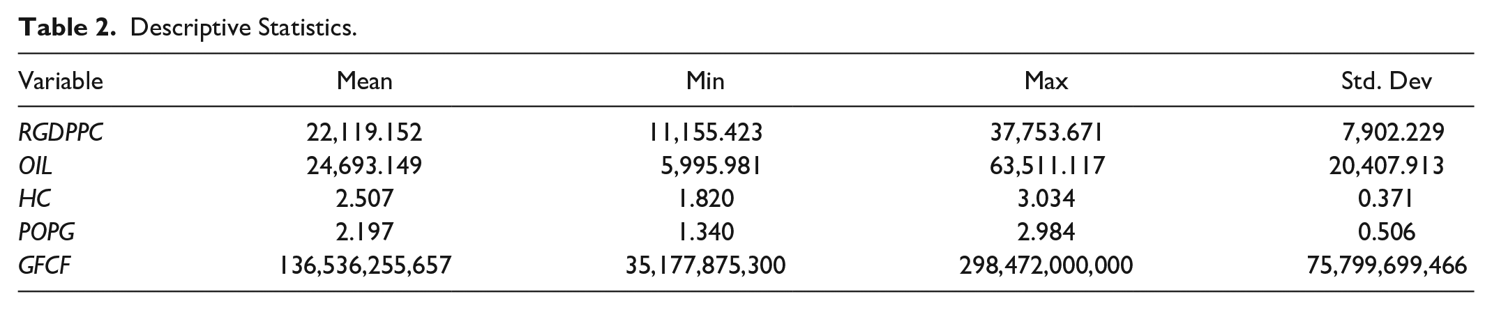
Table 2, on the other hand, provides a comprehensive descriptive statistic for the data set employed in this study. As seen in Table 2, the standard deviations of the variables are considerably discrete around the mean. The results imply that variations in those variables are resilient across the study sample. Specifically, this further inspires this study to investigate if the variations in the prices of oil can justify the differences in the real income levels, which is the primary concern of this study to be addressed.

Table 2.

Descriptive Statistics.

Variable	Mean	Min	Max	Std. Dev
RGDPPC	22,119.152	11,155.423	37,753.671	7,902.229
OIL	24,693.149	5,995.981	63,511.117	20,407.913
HC	2.507	1.820	3.034	0.371
POPG	2.197	1.340	2.984	0.506
GFCF	136,536,255,657	35,177,875,300	298,472,000,000	75,799,699,466

Moreover, Table 3 provides the correlation analysis using the Pearson Correlation Coefficient to obtain a brief insight into the contemporaneous relationships between the variables. As demonstrated in Table 3, the OIL and RGDPPC variable have a correlation coefficient of .762. Nevertheless, correlation does not imply causation and hence should be interpreted with caution. If OIL indeed plays a crucial role in affecting real GDP per capita, one can expect that OIL may lead to having a significant effect. In addition, human capital (HC) and investment (GFCF) reveals a positive correlation with real GDP per capita while population growth (POPG) is negatively correlated with real GDP per capita, in conformity with the theory.

Table 3.

Pearson Correlation Results.

	RGDPPC	OIL	HC	POPG	GFCF
RGDPPC	1.000
OIL	.762^a	1.000
HC	.973^a	.767^a	1.000
POPG	−.914^a	−.794^a	−.840^a	1.000
GFCF	.962^a	.659^a	.906^a	−.865^a	1.000

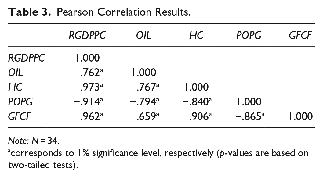
Note: N = 34.

corresponds to 1% significance level, respectively (p-values are based on two-tailed tests).

Results and Discussion

The estimation outcomes for the linear as well as the nonlinear ARDL models are presented in Tables 5 to 8. Table 4 presents the results of the unit root test, which is a pre-requisite test in the ARDL bounds test. The results are estimated by limiting the number of lags to four on the model, and the optimum number of lags is ascertained using the Schwarz Information Criterion (SIC), which appear to be more appropriate for analyses with small sample sizes. This preference stem from the idea that it would be more logical to have shorter lags for a shorter span of data. The maximum lag set will be four lags for the dependent and independent variables, where possible, provided there is no degree of freedom issue. Nevertheless, the maximum number of lags will be minimized if the chosen model suffers from serial correlation issues, as suggested by Pesaran et al. (2001).

Table 4.

Unit Root Test Results.

Variables	ADF test results		KPPS test results
Variables	Without trend	With trend	Without trend	With trend
	Level
LnRGDPPC	−0.42 (0)	−1.76 (0)	0.72 (5)^b	0.12 (4)^c
LnOIL	−1.08 (0)	−1.70 (1)	0.60 (5)^b	0.10 (4)
LnHC	−2.66 (1)^c	−1.83 (1)	0.71 (5)^b	0.19 (5)^b
LnPOPG	0.21 (7)	−3.48 (7)^c	0.62 (5)^b	0.19 (4)^b
LnGFCF	−0.78 (0)	−1.75 (0)	0.65 (5)^b	0.10 (4)
	First difference
∆LnRGDPPC	−4.99 (0)^a	−4.91 (0)^a	0.07 (1)	0.07 (1)
∆LnOIL	−4.80 (0)^a	−4.76 (0)^a	0.17 (2)	0.15 (2)^b
∆LnHC	−0.95 (0)	−2.20 (0)	0.64 (5)^b	0.09 (4)
∆LnPOPG	−2.34 (5)	−1.78 (6)	0.32 (4)	0.08 (2)
∆LnGFCF	−4.24 (0)^a	−4.18 (0)^b	0.06 (1)	0.06 (1)

Notes: Numbers inside parentheses are the optimum lag order using the Schwarz Information Criterion (SIC) and the selection of bandwidth based on the Newey-West nonparametric plug-in method for the ADF test and KPSS test, respectively.

^{, b,} and ^c denote significance at 1%, 5%, and 10% level, respectively.

Unit Root tests

Prior to the bound testing approach, the determination of the variable’s order of integration is a must, where the variables must either be I(0), I(1) or fractionally integrated. The variables, however, cannot be I(2). Thus, the stationarity of the variables is determined by utilizing two-unit root tests, namely ADF and KPSS. Results for these tests are tabulated in Table 4. These results are an indication that the variables are either integrated of, I(0) or I(1). Given that this fulfils the criteria for ARDL bound test, hence this study can proceed with the estimation of the ARDL model.

ARDL Results: Linear Model

For this study, the estimation of the linear model is conducted to scrutinize the effects that change in the price of oil has on growth, where oil revenue is utilized as a proxy for the oil price. Table 5 presents the results for the linear model estimation, where Panel A comprises of the coefficients and the standard error for the unrestricted ECM, Panel B is the corresponding estimated augmented ARDL model’s diagnostic result, and Panel C consists of the lower bound and upper bound critical values of the three cointegration test applied in this study.

Table 5.

Linear ARDL Estimation Results and Diagnostic Checks.

Panel A: Coefficient estimates of linear ARDL (2, 2, 1, 1, 1)
Constant			1.618 (0.739)^b
LnRGDPPC_t-1			−0.465 (0.123)^a
LnOIL_t-1			0.006 (0.010)
LnHC _t-1			0.589 (0.201)^a
LnPOPG _t-1			−0.056 (0.039)
LnGFCF _t-1			0.099 (0.023)^a
∆LnRGDPPC_t-1			−0.180 (0.088)^c
∆LnOIL_t			0.009 (0.013)
∆LnOIL_t-1			−0.022 (0.015)
∆LnHC_t			−2.148 (1.394)
∆LnPOPG_t			0.243 (0.098)^b
∆LnGFCF_t			0.227 (0.022)^a
Panel B: Diagnostic results
ECT_t-1			−0.465 (0.088)^a
Adj. R²			0.999
LM(2)			2.160
Ramsey’s RESET test			1.421
CUSUM (CUSUMSQ)			S(S)
F-statistic (overall)			4.738
t-statistic (lagged DV)			−3.790
F-statistic (lagged IDV)			5.899
Panel C: Summary of the lower bound and upper bound critical values
	10%		5%		1%
	I(0)	I(1)	I(0)	I(1)	I(0)	I(1)
F-statistic (overall)	2.696	3.898	3.276	4.630	4.590	6.368
t-statistic (lagged DV)	−2.570	−3.660	−2.860	−3.990	−3.430	−4.600
F-statistic (lagged IDV)	2.140	3.820	2.700	4.670	4.030	6.630

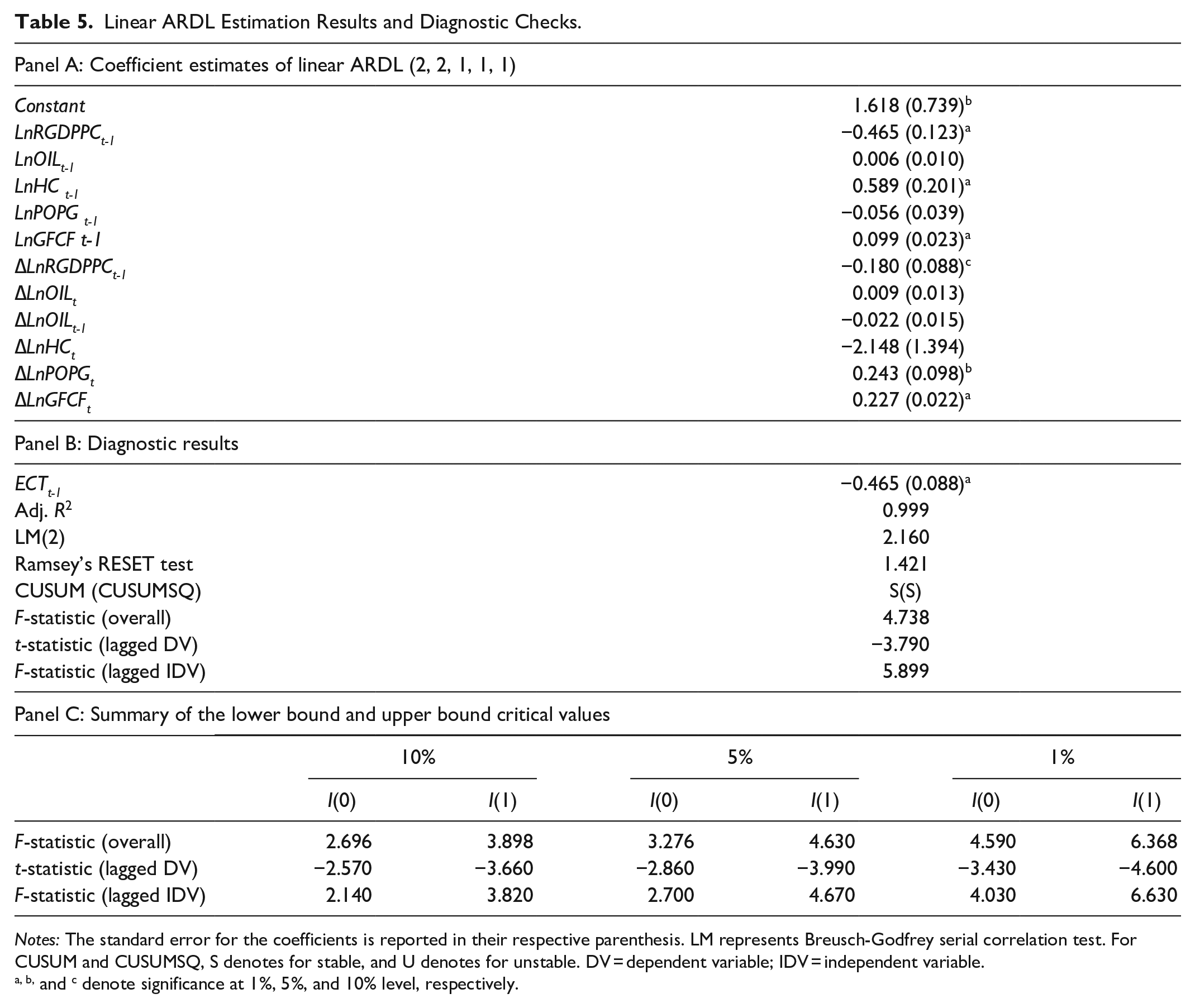
Notes: The standard error for the coefficients is reported in their respective parenthesis. LM represents Breusch-Godfrey serial correlation test. For CUSUM and CUSUMSQ, S denotes for stable, and U denotes for unstable. DV = dependent variable; IDV = independent variable.

^{, b,} and ^c denote significance at 1%, 5%, and 10% level, respectively.

Figures 2 and 3 shows the result of the cumulative sum (CUSUM) and cumulative sum of squares (CUSUMSQ) for the linear ARDL model, respectively. The selected model is free from autocorrelation and does not suffer from misspecification issues. As such, this study may proceed with the linear ARDL analysis.

Figure 2.

Plot of CUSUM for linear ARDL model.

Figure 3.

Plot of CUSUMSQ for linear ARDL model.

The initial phase of the analytical process involves establishing whether the variables employed in this growth model are cointegrated. Based on the computed overall F-statistic of 4.738, this study rejects the null hypothesis of no cointegration at the 5% significance level based on the Narayan (2005) critical value. The t-statistic of −3.790, however, lies between the lower bound and upper bound critical values provided by Pesaran et al. (2001) at 5% significance level, thus leading to an inconclusive result. As for the F-statistic for lagged independent variables as suggested by McNown et al. (2018), the computed F-statistic of 5.899 is greater than the upper bound critical value. Overall, results indicate a degenerate lagged dependent variable case, and thus, there is no cointegration among the variables (see Goh et al., 2017; McNown et al., 2018). The results for the long-run estimation are presented in Table 6. These results, however, are meaningless as cointegration cannot be established among the variables. By comparison, the study conducted by Maji et al. (2017) found that the effect of oil price is positively significant on the economic growth, such that a decline in oil prices, lowers the GDP of Malaysia.

Table 6.

Long-Run Results.

LnOIL	0.013 (0.022)
LnHC	1.266 (0.208)^a
LnPOPG	−0.120 (0.070)^c
LnGFCF	0.212 (0.039)^a

Notes: The standard error for the coefficients is reported in their respective parenthesis.

and ^c denote significance at 1% and 10% level, respectively.

Looking at the results obtained so far, it is intriguing that a cointegrating relationship cannot be established for the case of Malaysia, despite Malaysia being a net oil-exporting nation, which relies on oil revenue for its national development agenda. It is, therefore, likely that modeling the oil price and macroeconomic variables in a linear configuration could be inappropriate (Farzanegan & Markwardt, 2009; Moshiri & Banihashem, 2012). These leads to the possibility that such results could be due to the assumption of symmetric effect. As such, the possibility of asymmetric effect is explored in the following section to elucidate the nexus of oil shocks and Malaysian economic growth.

ARDL Results: Nonlinear Model

Since cointegration cannot be established through a linear ARDL model, a NARDL model is employed to determine if the movements in the price of oil have an asymmetric effect on the growth of the Malaysian economy instead. However, to proceed with the estimation process, the changes in the oil revenue are first decomposed into POS and NEG. Both the POS and NEG variables will then substitute the LnOIL variable in estimating the asymmetric effect, also known as the NARDL model. The results are displayed in Table 7, where Panel A consists of the coefficients and the standard error for the unrestricted ECM. At the same time, Panel B is the corresponding estimated NARDL model’s diagnostic result, and Panel C consists of the lower bound and upper bound critical values of the three cointegration test applied in this study.

Table 7.

Nonlinear ARDL Estimation Results and Diagnostic Checks.

Panel A: Coefficient estimates of NARDL (1, 0, 1, 1, 1, 2)
Constant			2.367 (0.715)^a
LnRGDPPC_t-1			−0.703 (0.153)^a
POS_t-1			0.036 (0.018)^c
NEG_t-1			−0.038 (0.020)^c
LnHC _t-1			0.521 (0.197)^b
LnPOPG _t-1			−0.021 (0.042)
LnGFCF _t-1			0.162 (0.038)^a
∆POS_t			0.036 (0.018)^c
∆NEG_t			−0.030 (0.026)
∆LnHC_t			−3.817 (1.554)^b
∆LnPOPG_t			0.197 (0.099)^c
∆LnGFCF_t			0.231 (0.020)^a
∆LnGFCF_t-1			−0.057 (0.022)^b
Panel B: Diagnostic results
ECT_t-1			−0.703 (0.112)^a
SUM POS SR			0.036 (0.018)^c
SUM NEG SR			−0.030 (0.026)
W_SR			0.066 (0.038)^c
W_LR			0.074 (0.035)^b
Adj. R²			0.999
LM(2)			2.570
Ramsey’s RESET test			2.880
CUSUM (CUSUMSQ)			S(S)
F-statistic (overall)			5.394
t-statistic (lagged DV)			−4.593
F-statistic (lagged IDV)			6.459
Panel C: Summary of the lower bound and upper bound critical values
	10%		5%		1%
	I(0)	I(1)	I(0)	I(1)	I(0)	I(1)
F-statistic (overall)	2.696	3.898	3.276	4.630	4.590	6.368
t-statistic (lagged DV)	−2.570	−3.660	−2.860	−3.990	−3.430	−4.600
F-statistic (lagged IDV)	2.140	3.820	2.700	4.670	4.030	6.630

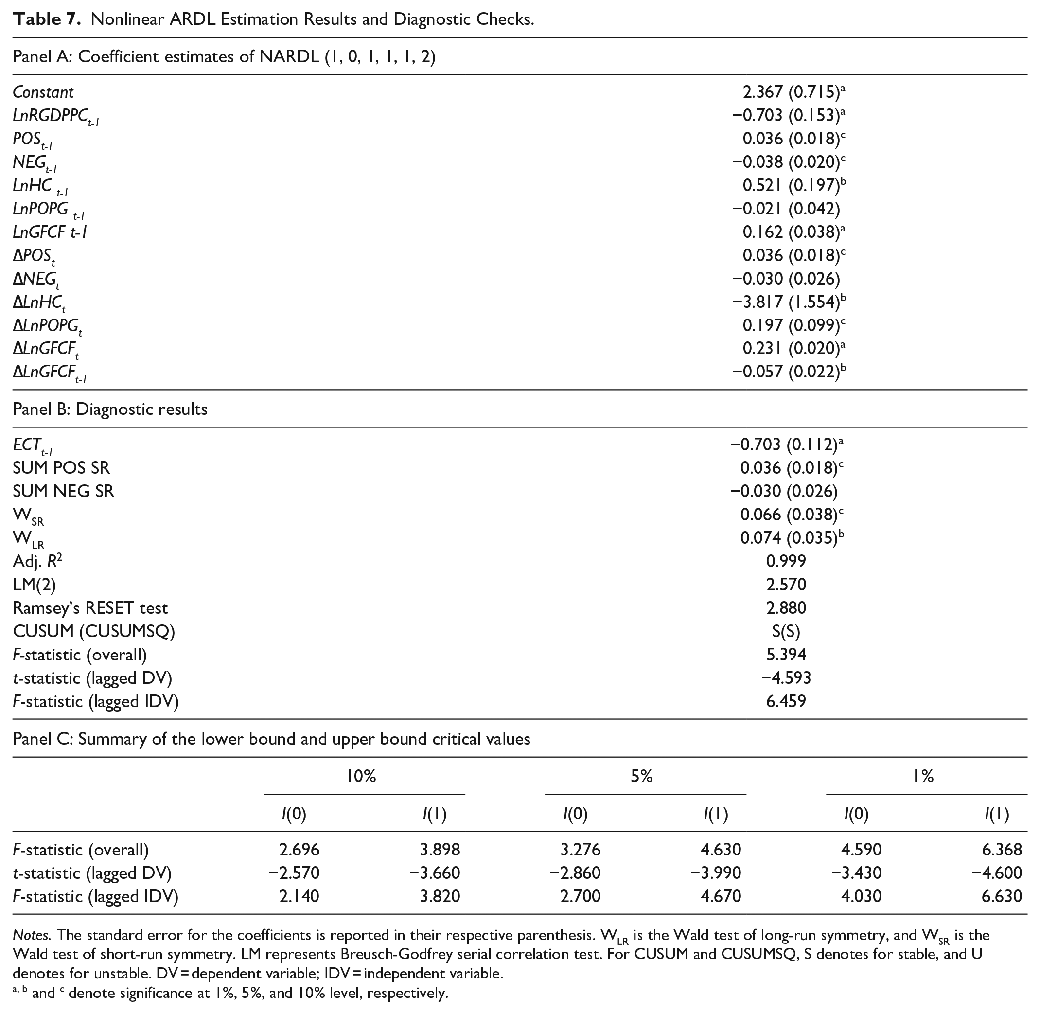
Notes. The standard error for the coefficients is reported in their respective parenthesis. W_LR is the Wald test of long-run symmetry, and W_SR is the Wald test of short-run symmetry. LM represents Breusch-Godfrey serial correlation test. For CUSUM and CUSUMSQ, S denotes for stable, and U denotes for unstable. DV = dependent variable; IDV = independent variable.

^{, b} and ^c denote significance at 1%, 5%, and 10% level, respectively.

Similar to the ARDL procedure, the presence of cointegration must first be established. The results for the three cointegration tests are reported in Panel B of Table 7. From the results obtained, the computed overall F-statistic is significant at the 5% level. As such, the t-statistic for lagged dependent variable and F-statistic for lagged independent variables are computed. Both the t-statistic for lagged dependent variable and F-statistic for lagged independent variables are both significant at 5% level. Results suggest that a cointegrating relationship exists for Malaysia in the long-run, using a NARDL model.

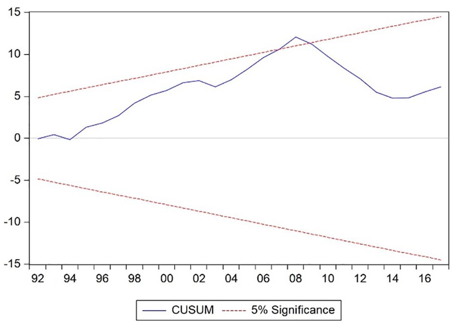
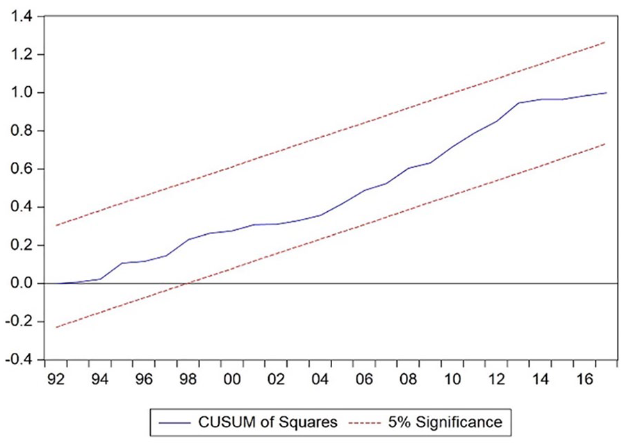
Additionally, a series of diagnostic tests are conducted, and the estimated models are deemed as well specified, fulfilling conditions of no autocorrelation and misspecification issues. The CUSUM and CUSUMSQ tests also found to be adequately stable at the 5% significance level. Figures 4 and 5 shows the result of the CUSUM and CUSUMSQ for the nonlinear ARDL model respectively. Also, the goodness of fit, as indicated by the high values of adjusted R-squared (Adj. R²), demonstrates that the estimated model to the data is found to be satisfactory. This further validates that the estimated growth model can provide a satisfactory interpretation of the behavior of the Malaysian economic progress.

Figure 4.

Plot of CUSUM for nonlinear ARDL model.

Figure 5.

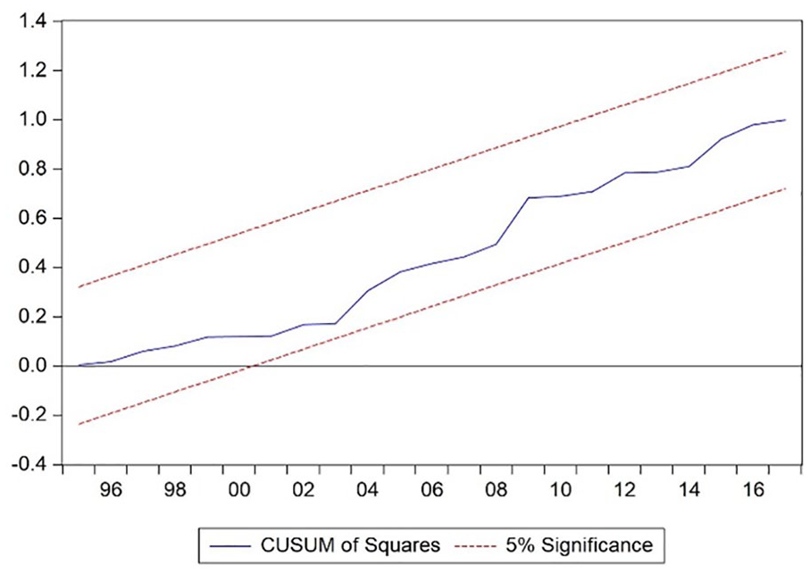
Plot of CUSUMSQ for nonlinear ARDL model.

To test whether the oil shocks are indeed asymmetric, the Wald tests of short-run and long-run symmetry is then applied. The results of the calculated Wald test are displayed in Panel B of Table 7. The results demonstrate that the oil shocks in the short-run (W_SR) is deemed to be statistically insignificant at the 5% significance level, indicating the non-existence of the short-run asymmetric effect of oil shocks. On the other hand, the Wald test (W_LR) implies that in the long-run, oil shocks have asymmetric effects. This supports the presence of the nonlinear relationship within the oil price-growth relationship, specifically for the case of Malaysia. The results are also in agreement with Moshiri and Banihashem (2012), Donayre and Wilmot (2016), and Nusair (2016) who documented that the growth effect of oil price shocks seems to be well explained using the asymmetric effect, particularly on the oil-exporting nations. This result however differs from the works of Kriskkumar and Naseem (2019) and Khan et al. (2019), who found that a nonlinear relationship between oil price and economic growth is not present in the case of Malaysia, using the NARDL model. However, it is worth noting that these studies use oil price instead of oil revenue when regressing, which led to a different result.

In the interim, results of the long-run estimates of the nonlinear ARDL model are presented in Table 8. Both the POS and NEG variable carries a significant coefficient. The POS coefficient indicates that a 1% increase in the oil revenue leads to approximately 0.051% improvement in output progress. The result implies that an increase in oil prices appears to benefit the Malaysian economy. This is consistent with the theoretical prediction that an increase in oil price will be beneficial for the economic growth of oil-exporting countries like Malaysia. When an oil price increase, it translates to an increase in oil revenue as well. These increase in oil revenue can then be used by the government to finance their expenditures and invest it in the development of the country, resulting in economic growth. In comparison the study conducted by Aziz and Dahalan (2015), found that positive changes in the oil price affects the output growth negatively. As it is a panel data analysis, it is hardly surprising if the results are different.

Table 8.

Long-Run Results.

POS	0.051 (0.020)^b
NEG	−0.054 (0.025)^b
LnHC	0.742 (0.256)^a
LnPOPG	−0.030 (0.060)
LnGFCF	0.231 (0.028)^a

Notes. The standard error for the coefficients is reported in their respective parenthesis.

and ^b denote significance at 1% and 5% level, respectively.

The NEG coefficient, on the other hand, indicates that a 1% decrease in the oil price leads to a 0.054% improvement in the output progress. This implies that a decrease in oil prices appears to benefit the Malaysian economy as well. Such phenomena seem to be appropriate as the supply of goods that are produced using energy are impacted directly by the price of crude oil, in which a decrease in oil price is projected to increase productivity and national output. This defies Hamilton’s (2011) model, where an increase in oil price leads to a decline in productivity due to an exogenous decrease in the supply. At the same time, a decrease in oil price shocks would also mean an increase in the exports of Malaysia. Given that declining oil price may place downward pressure on the Malaysian ringgit, leading to higher demand for exports such that outweighs the loss of lower export earnings from oil exports. The surge in exports volume may be due to trading partners, which now tend to buy more goods from Malaysia as it is relatively cheaper and more competitive in the international market, thereby contributing to the economic progress of Malaysia.

These results indicate that the asymmetric effect of oil price on the economic growth in Malaysia does not stem from unfavorable conditions such as the appreciation of exchange rates (so-called Dutch disease), rent-seeking activities and poor policy-making decisions, as posit by Moshiri and Banihashem (2012). Typically, the boom in commodity prices and revenue leads to be channeled to a non-productive public investment, which often generates minimal, zero or even negative returns (Talvi & Vegh, 2000). However, this is not the case for Malaysia. When the oil price increase, we find that Malaysia is capable of utilizing this gain to improve the economic growth of the country. An increase in the price of oil would boost the national coffers through the oil revenue channel. The increase in the revenue of oil could potentially contribute to the economic development of Malaysia, provided that the oil revenues are being managed efficiently and effectively. Investment in large development projects or high return projects prudently will ensure the maximization of oil revenue in developing the country. In some cases, an increase in the prices of oil may not necessarily lead to positive growth in the economy of a country. However, Malaysia does not fall into this category.

At the same time, when the oil price decrease, the economic growth of the country is also increasing as well. Given that crude oil is also one of the vital sources of input in production, a reduction in the cost of manufacturing would mean that suppliers would now be able to reduce their prices. This leads to a positive impact on Malaysian export expansion strategy through the increase in its production process. Besides, the declining oil price could also be fruitful to economic growth as it may improve economic conditions through the competitiveness effect of exchange rate depreciation. This leads to a better competitive level of local goods and services, in which it may become relatively cheaper in the international market, resulting in higher spending on those goods and services, and contribute to the economic progress of Malaysia. This suggests that Malaysia can take advantage of both the increase and decrease in oil price in developing the economy.

Robustness Checks

The sensitivity of the estimated model is further ascertained through the robustness checks, in which alternate measurement of oil price is used. For robustness checks, the oil revenue variable is substituted with the constant 2010 US Dollars real Brent crude oil, BRENT, obtained from World Bank Commodity Price Data. Brent crude oil price is commonly employed in the literature as a significant portion of the global oil trade, as much as 70%, is priced from the Brent basket, both directly and indirectly, making it a leading benchmark for the price of crude oil (Fattouh, 2011). Table 9 tabulates the estimated results for the robustness model, where Panel A consists of the coefficients and the standard error for the unrestricted ECM. At the same time, Panel B is the corresponding estimated ARDL and NARDL model’s diagnostic result, and Panel C consists of the lower bound and upper bound critical values of the three cointegration test applied in this study. Results for the long-run estimates are presented in Table 10.

Table 9.

Robustness Test.

			Linear model		Nonlinear model
Panel A: Coefficient estimates of unrestricted error-correction models
Selected Model			(1, 1, 1, 2, 1)		(2, 0, 1, 1, 1, 0)
Constant			2.567 (0.694)^a		2.576 (0.656)^a
LnRGDPPC_t-1			−0.572 (0.149)^a		−0.800 (0.083)^a
LnBRENT_t-1			−0.002 (0.001)
POS_t-1					0.055 (0.014)^a
NEG_t-1					−0.022 (0.014)
LnHC _t-1			0.810 (0.216)^a		0.604 (0.239)^b
LnPOPG _t-1			−0.120 (0.040)^a		−0.007 (0.045)
LnGFCF _t-1			0.099 (0.030)^a		0.188 (0.019)^a
∆LnBRENT_t			0.027 (0.012)^b
∆POS_t					0.055 (0.014)^a
∆NEG_t					0.025 (0.016)
∆LnHC_t			−1.589 (1.246)		−2.899 (1.209)^b
∆LnPOPG_t			0.219 (0.195)		0.458 (0.100)^a
∆LnGFCF_t			0.190 (0.021)^a		0.188 (0.019)^a
Panel B: Diagnostic results
ECT_t-1			−0.572 (0.106)^a		−0.800 (0.056)^a
SUM POS SR					0.055 (0.014)^a
SUM NEG SR					0.025 (0.016)
W_SR					0.029 (0.025)
W_LR					0.077 (0.022)^a
Adj. R²			0.999		0.999
LM(2)			2.756		3.313
Ramsey’s RESET test			0.098		3.310^c
CUSUM (CUSUMSQ)			S(S)		S(S)
F-statistic (overall)			4.949		28.552
t-statistic (lagged DV)			−3.837		−9.632
F-statistic (lagged IDV)			6.185		33.362
Panel C: Summary of the lower bound and upper bound critical values
	10%		5%		1%
	I(0)	I(1)	I(0)	I(1)	I(0)	I(1)
F-statistic (overall)	2.696	3.898	3.276	4.630	4.590	6.368
t-statistic (lagged DV)	−2.570	−3.660	−2.860	−3.990	−3.430	−4.600
F-statistic (lagged IDV)	2.140	3.820	2.700	4.670	4.030	6.630

Notes. The standard error for the coefficients is reported in their respective parenthesis. LM is the Breusch-Godfrey serial correlation test with the number of lags as stated in parenthesis. For CUSUM and CUSUMSQ, S stands for stable, and U stands for unstable.

^{, b,} and ^c denote significance at 1%, 5%, and 10% level, respectively.

Table 10.

Long-Run Results—Robust Model.

	Linear model	Nonlinear model
LnBRENT	−0.003 (0.016)
POS		0.068 (0.020)^a
NEG		−0.027 (0.018)
LnHC	1.415 (0.137)^a	0.755 (0.248)^a
LnPOPG	−0.209 (0.056)^a	−0.008 (0.056)
LnGFCF	0.174 (0.023)^a	0.235 (0.028)^a

Notes. The standard error for the coefficients is reported in their respective parenthesis.

indicates 1% significance level respectively.

For the linear model, the t-statistic on the lagged dependent variable is insignificant at 5% level, suggesting that a cointegrating relationship among the variables is absent. Moving to the nonlinear model, the three cointegrations tests are significant at the 1% level, indicating that a long-run relationship exists. The Wald test for short-run is insignificant at the 5% level, but the long-run symmetry returns significant results at the 1% level. This signifies that an asymmetric effect is present in the long-run and not in the short-run. Only the POS variable is significant in this model at the 1% level while the NEG variable turns out to be insignificant at the 5% significance level. This indicates that an increase in oil shocks by 1% results in approximately 0.068% increase in economic output in the long-run. The diagnostic tests for both the linear and nonlinear model are found to be adequate in elucidating the following model of Malaysian economic growth. Figures 6 and 7 shows the result of the CUSUM and CUSUMSQ for the robust linear ARDL model respectively, while Figures 8 and 9 shows the result of the CUSUM and CUSUMSQ for the robust nonlinear ARDL model respectively.

Figure 6.

Plot of CUSUM for robust linear ARDL model.

Figure 7.

Plot of CUSUMSQ for robust linear ARDL model.

Figure 8.

Plot of CUSUM for robust nonlinear ARDL model.

Figure 9.

Plot of CUSUMSQ for robust nonlinear ARDL model.

The results from the robustness test are not entirely identical as the use of Brent crude oil price may result in inaccurate analysis. This inaccuracy stems from the idea that some oil-exporting countries may increase their exports when the oil price is low to obtained back higher revenue from the oil sector for better economic growth (Moshiri & Banihashem, 2012). Despite that, this result supports the main findings, which validate the significant role, played by the oil shocks, particularly in an economic growth-enhancing effect. Furthermore, it validates the significance of an asymmetric effect in the oil prices-growth nexus. Therefore, the empirical results are robust to the alternative model specification and proxy of growth.

Conclusions and Policy Implications

This study investigates the asymmetric effect of oil price on the economic growth of Malaysia. The augmented ARDL framework is used to scrutinize the linear effects before proceeding with a NARDL model to establish the presence of asymmetric effect within the oil price-economic growth framework. The linear ARDL model indicates that cointegration is not present in the Malaysian case while the NARDL model exhibits a clear presence of the long-run asymmetric effect of oil prices on the Malaysian economic growth. This substantiates the claim that the linkage between economic growth and the price of oil appeared to be nonlinear. Additionally, the positive changes in oil prices, POS has a significant positive coefficient, while the negative changes in oil prices, NEG has a significant negative coefficient. Such findings are intriguing, given that both positive and negative changes in the oil prices contribute to the economy of a net oil-exporter like Malaysia instead of having polar opposite effects.

The evidence in this paper has shed some light on the “oil price-growth puzzle” in the case of Malaysia. First, the oil price-growth nexus in Malaysia is complex and cannot be explained merely from a linear perspective. Second, the negative impact of oil prices is not felt by Malaysia, as both increase and decrease in oil prices positively impact Malaysia’s economic growth. Such favorable condition can be attributed to the efficiency and effectiveness of the Malaysian authorities in dealing with changes in oil prices. An espousal of income assistance such as cash aid to the low-income group (B40) and tax relief measures coupled with accommodative monetary policies have helped Malaysia overcome the adverse effects of lower oil prices. On the other hand, suppliers and entrepreneurs were clearly able to take advantage of the lower oil prices while also protecting themselves from rising oil prices through hedging and effective cost-cutting measures.

While it is clear that Malaysia’s economy has a strong resilience toward volatility of oil prices, it should not be too complacent with what it has achieved so far. There are several measures on which Malaysia should focus. First, consideration for future policies should comprise appropriate efforts to reduce dependency on oil and gas sectors. Crude oil is non-renewable energy, and as such, it is only a matter of time before this natural resource is depleted. With that in mind, Malaysia should be cautious in being too dependent on crude oil as a source of income. As the world moves toward a green economy, Malaysia should consider generating cleaner electrical energy using solar panels. Malaysia could also promote the use of electric cars in Malaysia by providing incentives to car automakers to manufacture and sell electric cars in Malaysia. Furthermore, a reduction in dependency on the oil and gas sector would also contribute to a pollution-free environment. Second, Malaysia should continue with its diversification programs. With most nations in the arms race in the fourth industrial revolution, Malaysia cannot afford to be left behind in this race. The recent Malaysia Digital Economy Blueprint comes as good news for Malaysia, as it shows the initiative Malaysia is taking in making headway in the new industry. However, following the trend of digitalization alone will not be enough. Malaysia should couple it with innovation in the tech sector in order to have a chance at competing with other nations. For future research on the oil price-growth nexus, it would be intriguing to see how the exchange rate component affects the complex relationship between oil price and economic growth.

Footnotes

Declaration of Conflicting Interests

The author(s) declared no potential conflicts of interest with respect to the research, authorship, and/or publication of this article.

Funding

The author(s) disclosed receipt of the following financial support for the research, authorship, and/or publication of this article: This study was funded by the Ministry of Education Malaysia under the FRGS scheme with the title Searching for GDP-Stabilizing Model in the Presence of Oil Price Shock (Grant no. FRGS/1/2019/SS08/UPM/02/4).

Ethical Approval

This article does not contain any studies with human participants or animals performed by any of the authors.

ORCID iDs

Karunanithi Kriskkumar

Niaz Ahmad Mohd Naseem

References

Abdlaziz

R. A.

Naseem

N. A.

Slesman

(2022). Oil revenue and agriculture value-added in oil-exporting countries: Does the role of real exchange rate matter? International Journal of Energy Sector Management, 16, 171–190. https://doi.org/10.1108/ijesm-11-2020-0006

Abdlaziz

Naseem

N. A. M.

Slesman

Ahmed

(2021). The impact of oil price shocks on the military expenditure of selected MENA oil exporting countries: Symmetric and asymmetric cointegration analysis. Iranian Economic Review, 25(2), 219–235. https://doi.org/10.22059/ier.2021.83447

Auty

(1993). Sustaining Development in Mineral Economies: The Resource Curse Thesis (1st ed.). Routledge.

Aziz

M. I. A.

Dahalan

(2015). Oil Price Shocks and macroeconomic activities in asean-5 countries: A panel VAR approach. Eurasian Journal of Business and Economics, 8, 101–120. https://doi.org/10.17015/ejbe.2015.016.06

Azman-Saini

W. N.

Baharumshah

A. Z.

Law

S. H.

(2010). Foreign direct investment, economic freedom and economic growth: International evidence. Economic Modelling, 27(5), 1079–1089. https://doi.org/10.1016/j.econmod.2010.04.001

Bala

Chin

(2020). Asymmetric impacts of oil price shocks on Malaysian economic growth: Nonlinear autoregressive distributed lag approach. Iranian Economic Review, 24(4), 959–981. https://doi.org/10.22059/ier.2020.78830

Berument

M. H.

Ceylan

Dogan

(2010). The impact of oil price shocks on the economic growth of selected MENA1 countries. The Energy Journal, 31, 149–176. https://doi.org/10.5547/issn0195-6574-ej-vol31-no1-7

Bloom

D. E.

Canning

Sevilla

(2004). The effect of health on economic growth: A production function approach. World Development, 32(1), 1–13. https://doi.org/10.1016/j.worlddev.2003.07.002

Bouoiyour

Selmi

Tiwari

A. K.

Shahbaz

(2015). The nexus between oil price and Russia’s real exchange rate: Better paths via unconditional vs conditional analysis. Energy Economics, 51, 54–66. https://doi.org/10.1016/j.eneco.2015.06.001

10.

Campos

N. F.

(2001). Will the future be better tomorrow? The growth prospects of transition economies revisited. Journal of Comparative Economics, 29(4), 663–676. https://doi.org/10.1006/jcec.2001.1741

11.

Charfeddine

Barkat

(2020). Short- and long-run asymmetric effect of oil prices and oil and gas revenues on the real GDP and economic diversification in oil-dependent economy. Energy Economics, 86, 104680. https://doi.org/10.1016/j.eneco.2020.104680

12.

Cheng

Liu

(2020). Natural resource abundance, resource industry dependence and economic green growth in China. Resources Policy, 68, 101734. https://doi.org/10.1016/j.resourpol.2020.101734

13.

Corden

W. M.

Neary

J. P.

(1982). Booming sector and de-industrialisation in a small open economy. The Economic Journal, 92(368), 825–848. https://doi.org/10.2307/2232670

14.

Donayre

Wilmot

N. A.

(2016). The asymmetric effects of oil price shocks on the Canadian economy. International Journal of Energy Economics and Policy, 6(2), 167–182. https://doi.org/10.2139/ssrn.2567576

15.

Eia

(2019). International Energy Statistics. US Energy Information Administration. https://www.eia.gov/beta/international/data/browser/

16.

Elder

Serletis

(2010). Oil Price Uncertainty. Journal of Money Credit and Banking, 42(6), 1137–1159. http://www.jstor.org/stable/40784879

17.

Eltony

M. N.

Al-Awadi

(2001). Oil price fluctuations and their impact on the macroeconomic variables of Kuwait: A case study using a VAR model. International Journal of Energy Research, 25(11), 939–959. https://doi.org/10.1002/er.731

18.

Engle

R. F.

Granger

C. W. J.

(1987). Co-integration and error correction: Representation, estimation, and testing. Econometrica, 55(2), 251–276. https://doi.org/10.2307/1913236

19.

Farzanegan

M. R.

Markwardt

(2009). The effects of oil price shocks on the Iranian economy. Energy Economics, 31(1), 134–151. https://doi.org/10.1016/j.eneco.2008.09.003

20.

Fattouh

(2011). An anatomy of the crude oil pricing system. Oxford Institute for Energy Studies WPM. https://ora.ox.ac.uk/objects/uuid:8b957970-239c-4a4f-9cbe-21830381de16

21.

Frankel

(1962). The production function in allocation and growth: A synthesis. American Economic Review, 52(5), 996–1022. http://www.jstor.org/stable/1812179

22.

Frankel

J. A.

(2010). The natural resource curse: A survey (Working Paper Series, No. 15836). National Bureau of Economic Research. https://doi.org/10.3386/w15836

23.

Goh

S. K.

Yong

J. Y.

Lau

C. C.

Tang

T. C.

(2017). Bootstrap ARDL on energy-growth relationship for 22 OECD countries. Applied Economics Letters, 24(20), 1464–1467. https://doi.org/10.1080/13504851.2017.1284980

24.

Hamilton

J. D.

(1983). Oil and the macroeconomy since world war II. Journal of Political Economy, 91(2), 228–248. http://www.jstor.org/stable/1832055

25.

Hamilton

J. D.

(1996). This is what happened to the oil price-macroeconomy relationship. Journal of Monetary Economics, 38(2), 215–220. https://doi.org/10.1016/s0304-3932(96)01282-2

26.

Hamilton

J. D.

(2011). Historical oil shocks (Working Paper Series, Issue 16790). https://doi.org/10.3386/w16790

27.

Ito

(2017). Dutch disease and Russia. International Economics, 151, 66–70. https://doi.org/10.1016/j.inteco.2017.04.001

28.

Jiménez-Rodríguez

Sánchez

(2005). Oil price shocks and real GDP growth: empirical evidence for some OECD countries. Applied Economics, 37(2), 201–228. https://doi.org/10.1080/0003684042000281561

29.

Johansen

Juselius

(1990). Maximum Likelihood estimation and inference on Cointegration - with applications to the demand for money. Oxford Bulletin of Economics and Statistics, 52(2), 169–210. https://doi.org/10.1111/j.1468-0084.1990.mp52002003.x

30.

Khan

M. A.

Husnain

M. I. U.

Abbas

Shah

S. Z. A.

(2019). Asymmetric effects of oil price shocks on Asian economies: A nonlinear analysis. Empirical Economics, 57(4), 1319–1350. https://doi.org/10.1007/s00181-018-1487-7

31.

Korhonen

Mehrotra

A. N.

(2009). Real exchange rate, output and oil: Case of four large energy producers.Bank of Finland Institute for Economies in Transition (BOFIT) Discussion Paper 6/09. https://doi.org/10.2139/ssrn.1428238

32.

Kose

Baimaganbetov

(2015). The asymmetric impact of oil price shocks on Kazakhstan macroeconomic dynamics: A structural vector autoregression approach. International Journal of Energy Economics and Policy, 5(4), 1058–1064.

33.

Kriskkumar

Naseem

N. A. M.

(2019). Analysis of oil price effect on economic growth of ASEAN net oil exporters. Energies, 12(17), 3343. https://doi.org/10.3390/en12173343

34.

Lee

Ratti

R. A.

(1995). Oil shocks and the macroeconomy: The role of price variability. The Energy Journal, 16(4), 39–56. http://www.jstor.org/stable/41322616

35.

Levine

Renelt

(1992). A sensitivity analysis of cross-country growth regressions. American Economic Review, 82(4), 942–963. http://www.jstor.org/stable/2117352

36.

Mah

J. S.

(2000). An empirical examination of the disaggregated import demand of Korea—The case of information technology products. Journal of Asian Economics, 11(2), 237–244. https://doi.org/10.1016/s1049-0078(00)00053-1

37.

Maji

I. K.

Saari

M. Y.

Habibullah

M. S.

Utit

(2017). Measuring the economic impacts of recent oil price shocks on oil-dependent economy: Evidence from Malaysia. Policy Studies, 38(4), 375–391. https://doi.org/10.1080/01442872.2017.1320706

38.

Mankiw

N. G.

Romer

Weil

D. N.

(1992). A contribution to the empirics of economic growth. The Quarterly Journal of Economics, 107(2), 407–437. https://doi.org/10.2307/2118477

39.

McNown

Sam

C. Y.

Goh

S. K.

(2018). Bootstrapping the autoregressive distributed lag test for cointegration. Applied Economics, 50(13), 1509–1521. https://doi.org/10.1080/00036846.2017.1366643

40.

Mork

K. A.

(1989). Oil and the macroeconomy when prices go up and down: An extension of Hamilton’s results. Journal of Political Economy, 97(3), 740–744. http://www.jstor.org/stable/1830464

41.

Moshiri

Banihashem

(2012). Asymmetric effects of oil price shocks on economic growth of oil-exporting countries (Working Paper No. 12-140). USAEE. https://doi.org/10.2139/ssrn.2163306

42.

Narayan

P. K.

(2005). The saving and investment nexus for China: Evidence from cointegration tests. Applied Economics, 37(17), 1979–1990. https://doi.org/10.1080/00036840500278103

43.

Naseer

C.-W.

Mirza

J.-P.

(2020). Double jeopardy of resources and investment curse in South Asia: Is technology the only way out? Resources Policy, 68, 101702. https://doi.org/10.1016/j.resourpol.2020.101702

44.

Nusair

S. A.

(2016). The effects of oil price shocks on the economies of the Gulf Co-operation Council countries: Nonlinear analysis. Energy Policy, 91, 256–267. https://doi.org/10.1016/j.enpol.2016.01.013

45.

Olayungbo

D. O.

(2019). Effects of oil export revenue on economic growth in Nigeria: A time varying analysis of resource curse. Resources Policy, 64, 101469. https://doi.org/10.1016/j.resourpol.2019.101469

46.

Olomola

Adejumo

(2006). Oil price shock and macroeconomic activity in Nigeria. International Journal of Financial Research, 3(1), 28–34.

47.

Papyrakis

Gerlagh

(2004). The resource curse hypothesis and its transmission channels. Journal of Comparative Economics, 32(1), 181–193. https://doi.org/10.1016/j.jce.2003.11.002

48.

Pesaran

M. H.

Shin

Smith

R. J.

(2001). Bounds testing approaches to the analysis of level relationships. Journal of Applied Economics, 16(3), 289–326. https://doi.org/10.1002/jae.616

49.

Qadri

F. S.

Waheed

(2014). Human capital and economic growth: A macroeconomic model for Pakistan. Economic Modelling, 42, 66–76. https://doi.org/10.1016/j.econmod.2014.05.021

50.

Romer

P. M.

(1986). Increasing returns and long-run growth. Journal of Political Economy, 94(5), 1002–1037. https://doi.org/10.1086/261420

51.

Sam

C. Y.

McNown

Goh

S. K.

(2019). An augmented autoregressive distributed lag bounds test for cointegration. Economic Modelling, 80, 130–141. https://doi.org/10.1016/j.econmod.2018.11.001

52.

Sharma

S. S.

(2010). The relationship between energy and economic growth: Empirical evidence from 66 countries. Applied Energy, 87(11), 3565–3574. https://doi.org/10.1016/j.apenergy.2010.06.015

53.

Shin

Greenwood-Nimmo

(2014). Modelling Asymmetric Cointegration and dynamic multipliers in a nonlinear ARDL framework. In Sickles

R. C.

Horrace

W. C.

(Eds.), Festschrift in honor of Peter Schmidt: Econometric Methods and Applications (pp. 281–314). Springer.

54.

Talvi

Vegh

C. A.

(2000). Tax base variability and procyclical fiscal policy (Working Paper Series, No. 7499). National Bureau of Economic Research. https://doi.org/10.3386/w7499

Investigating the Asymmetric Effect of Oil Price on the Economic Growth in Malaysia: Applying Augmented ARDL and Nonlinear ARDL Techniques

Abstract

Keywords

Introduction

Background and Literature Review

Methodology

Model Specification

Econometric Methodology

Augmented Autoregressive Distributed Lag (ARDL) Model

Nonlinear Autoregressive Distributed Lag (NARDL) Model

Data

Results and Discussion

Unit Root tests

ARDL Results: Linear Model

ARDL Results: Nonlinear Model

Robustness Checks

Conclusions and Policy Implications

Footnotes

Declaration of Conflicting Interests

Funding

Ethical Approval

ORCID iDs

References