Sage Journals: Discover world-class research

Abstract

In recent years, counties in the Intermountain West (Colorado, Idaho, Montana, Wyoming, and Utah) have experienced rapid population growth and housing development, and much of this growth is occurring outside of urban areas. Residential development often has negative impacts on farmlands, farm viability, and environmental services provided by working landscapes. We used county-level data to identify the association between the intensity and spatial patterns of residential settlement and trends in selected farm outcomes between 1997 and 2012 in the region. Results demonstrate that accounting for the spatial pattern or degree of fragmentation and clustering of rural and exurban residential development improves our ability to explain variation in county-level agricultural trends. We also found evidence of significant spatial dependencies among the counties in this region, which suggests that trends in one county are affected by development and agricultural activity in neighboring counties. Findings suggest that efforts to protect farming using growth management tools can work, but should focus on separation of agriculture and potentially conflicting land uses.

Keywords

geography social sciences agricultural trends Intermountain West population growth rural and exurban areas spatial patterns

Introduction

The Intermountain West (IW), which encompasses Colorado, Idaho, Montana, Wyoming, and Utah, has experienced rapid population growth and dramatic patterns of social, economic, and landscape change over the last 30 years (Hines, 2010; Krannich, Luloff, & Field, 2011; Travis, 2007). Although the region was historically dependent on farming, ranching, mining, and other extractive industries, it has experienced a steady transition to a “post-cowboy” economy, and many areas are now dominated by service-, government-, recreation-, and amenities-based sectors (Power & Barrett, 2011; Winkler, Field, Luloff, Krannich, & Williams, 2007). Through this process of regional change, peoples’ historical ties to the land—both through work and recreation—have been transformed (Keske, Bixler, Bastian, & Cross, 2017; Nelson, 2001).

The five states of the IW region comprise the majority of the “interior” West, and are dominated by high and relatively inaccessible rangelands and mountain ranges (mostly owned and managed by the federal government) interspersed with irrigated valleys in which most agriculture and urban development takes place on privately owned land (McNabb & Avers, 1994). Even though the majority of population growth has occurred within existing urbanized areas, a sizable amount of residential development has also taken place outside of the incorporated municipalities (Otterstrom & Shumway, 2003), particularly in counties with high natural amenities that are adjacent to metropolitan areas (McGranahan, 1999; Travis, 2007).

Previous work has linked overall rates of population density and growth at the county level to negative effects on a wide range of agricultural trends in the region (Jackson-Smith, Jensen, & Jennings, 2006). However, despite repeated calls for “smarter” growth policies to encourage greater clustering of new housing within or near existing urban areas, the adoption of growth management policies and programs has been uneven across this five-state region (McKinney & Harmon, 2002). Moreover, there has been little empirical research to test the hypothesis that managing the spatial location and arrangement of residential housing development improves the viability of farm enterprises.

This article fills that gap by exploring how different patterns of residential settlement have affected trends in the agricultural sector. We used county-level data to assess how information about spatial patterns of population and housing in exurban and rural (unincorporated) areas can explain variation in rates of change of three key indicators of farm sector well-being: farm numbers, cropland acres, and gross farm sales.

Agricultural Restructuring in the West

While population pressure and urban growth patterns can alter the viability of farming enterprises, agricultural trends in the West also reflect broader patterns of farm structural change in the United States including increasing output along with consolidation of production in the hands of fewer large commercial operations; the emergence of a bi-modal farm structure characterized by growth in numbers of both very large and very small (hobby or recreation) farms, and a decline in mid-sized operations; replacement of labor through mechanization; and growing reliance on off-farm income to support farm households (Cochrane, 1993; Hines, 2010; Lobao & Meyer, 2001).

These trends reflect strong economic and technological forces, such as increasing technical economies of scale, consolidation in the input supply and farm output processing sectors, and the growing role of global markets for agricultural commodities (Bonanno & Constance, 2006). Economic drivers are tempered by social factors, whereby the quality of life benefits associated with farming help explain the persistence of family-labor midsized farms and ranches in the face of below-market rates of return, as well the growth of “lifestyle” farming operations (Bartlett, 1993; Jackson-Smith, 1999, 2004).

Farm structural change can have significant impacts on farm families, rural communities, and working landscapes. The declining economic viability of mid-sized, full-time commercial farms has led to increased financial and psychological stress for farm operators and family members (Belyea & Lobao, 1990), and farm structural change has been linked to declines in local spending (Foltz & Zeuli, 2005) and in the quality and types of farm community social ties and patterns of engagement (Goldschmidt, 1978; Jackson-Smith & Gillespie, 2005). Declining local ownership and control of farmland can negatively affect the quality of social relationships and interactions within the community (Petrzelka, Ma, & Malin, 2013). Changes from farming and ranching to housing development can affect wildlife populations, open space and landscape amenities, and local government finances (Theobald, Miller, & Hobbs, 1997).

Impacts of Urban Proximity and Demographic Change on Agriculture

The links between demographic and economic changes and agricultural trends are complex. Residential development’s impact on agriculture depends on the varying role of different causal mechanisms. Increasing land consumption by non-farm uses contributes to increases in land prices, fragmentation of farm fields, and declines in the land used for farming (MacLaren, Kimball, Holmes, & Eisenbeis, 2005; Travis, 2007). Rising land prices and doubts about the long-term future of commercial agriculture in urbanizing areas can threaten a traditional agrarian sense of place (Keske et al., 2017) and contribute to an “impermanence syndrome” where farmers underinvest in their operations in anticipation of selling for development (Adelaja, Sullivan, & Hailu, 2011). As commercial farming activity declines, the loss of a critical mass of farm operations can affect the viability of local agribusinesses and infrastructure (Jackson-Smith, 2003). At the local level, exurban and rural housing growth has been shown to increase the cost of community services (Carruthers & Ulfarsson, 2008) and can generate conflicts between farmers and their non-farming neighbors (Daniels, 1999; Heinman, 1989) and competition for water (Gollehon & Quinby, 2000).

At the same time, proximity to urban areas can work as a selection mechanism that favors some types of agriculture over others. Bid-rent theory has been long used to explain why farms producing higher value and more capital-intensive agricultural commodities would be expected to persist in the face of urban expansion, while rising land prices would drive more land-extensive and lower value commodity producers farther away from urbanizing areas (Sinclair, 1967; von Thünen, 1966). Although most agricultural products are not consumed locally and are sold into national or global commodity markets, a growing market exists for farms that produce directly for local or regional urban customers (Jackson-Smith & Sharp, 2008; Low et al., 2015). When farm production is linked to local consumption and processing, proximity to transportation networks between the hinterland and the urban core can be an important determinant of effective “urban proximity” (Walker & Solecki, 1999). At the same time, decisions by rural land owners reflect both productive and consumptive uses of the land (Cadieux & Hurley, 2011). To the extent that agricultural landowners value their property for reasons that go beyond production of commodities (e.g., family tradition, access to natural amenities, etc.), the persistence of sub-commercial lifestyle farming and ranching operations can be common in the rural West.

The impact of housing growth and urban development on agriculture can be particularly acute in the IW because 46% of the IW land base is in public (mainly federal) ownership, where new development is generally not permitted (Headwaters Economics, 2012). This forces new residential growth to occur nearly exclusively on the privately owned parts of the landscape which were originally settled by pioneers in the 19th and early 20th century (Gude, Hansen, Rasker, & Maxwell, 2006). Not coincidentally, these are also the areas with comparatively flat topography, the most productive agricultural soils, and the best access to irrigation water. The most urban and rapidly growing counties in the region have seen the most negative trends in farming overall, though population growth is positively associated with changes in farm numbers (Jackson-Smith et al., 2006).

Spatial Configurations (Patterns) of Development

The impacts of population growth on agriculture are mediated by the location and spatial arrangement of new housing construction on the landscape. For example, growth within the boundaries of existing urbanized areas is less likely to cause challenges for agriculture, while growth that takes place within the working agricultural landscape is expected to have more noticeable effects. Because local leaders usually eschew strict land use planning or zoning, residential development in unincorporated rural and exurban jurisdictions in the region is characterized by relatively large lots and are scattered across the landscape (Theobald, 2001). This form of growth has been criticized for being less economically and ecologically efficient and produces a larger human footprint on the environment per capita and overall (Theobald, Gosnell, & Riebsame, 1996). For example, dispersed forms of development can fragment landscapes, disrupt natural habitats, change landforms and drainage networks, and introduce exotic and invasive species (Alberti, 2005).

In response, planners seeking to protect farm operations and preserve open space have proposed policies that would steer new development away from the most productive agricultural soils, and encourage new housing to cluster together on smaller lots in areas close to existing urban services and transportation networks (Compas, 2007). Approaches have included purchasing development rights from willing farmland owners, restricting the types of development allowed on agriculturally zoned parcels, rewarding developments that cluster housing and preserve open space by providing density bonuses, and limiting provision of public services to designated areas on the fringes of existing municipalities (Hersperger, 2006; MacLaren et al., 2005).

To evaluate whether these policy approaches can protect agriculture, it is necessary to develop indicators to capture both the density and spatial arrangements of housing development outside of urban areas. Fortunately, there has been considerable progress in detecting and characterizing low-density development in the last 20 years. Early work used Census housing counts at the block group level to identify locations with growing exurban forms of development in the United States (Berube, Singer, Wilson, & Frey, 2006). Clark, McChesney, Munroe, and Irwin (2009) used estimates of population density at the 30″ × 30″ scale from the global “LandScan” database to demonstrate the wide diversity of spatial configurations of exurban settlement surrounding metropolitan centers in the lower 48 states.

A growing number of scholars have used remote sensed data and metrics developed in the field of landscape ecology to characterize spatial patterns of urban growth and residential development. Traditionally, landscape pattern metrics have been used to quantify the shape and pattern of vegetation or ecological habitats (Gustafson, 1998; Hargiss, Bissonette, & David, 1998). In recent years, a number of scholars have used these landscape pattern metrics to characterize spatio-temporal patterns of human settlement (DiBari, 2007; Fagan, Meir, Carroll, & Wu, 2001; Irwin & Bockstael, 2007; Palmer, 2004; Weng, 2007).

A number of studies have explored the associations between different forms of development and indicators of ecosystem structure and function (Luck & Wu, 2002; Theobald et al., 1997). To our knowledge, few studies have explored the links between different spatial patterns of rural and exurban development and agricultural outcomes. Deng, Wang, Hong, and Qi (2009) used spatial landscape metrics to document the process leading to the transition of an agricultural area to an urban-dominated landscape in China. Gude et al. (2006) showed that new rural and exurban housing development in the West is disproportionately located on productive soils and near water sources that are important to commercial agriculture.

Method

Approach

To better understand the associations between spatial patterns of residential settlement and farm trends at the county level in the IW, we combined data from multiple sources to capture the role of a range of drivers of agricultural outcomes. Given previous research, we expected that population pressure, local socioeconomic opportunity structure, and the quality of local biophysical resources would influence the nature and trajectory of changes in agriculture in the IW. To this basic model of farm change, we added a new variable—the spatial pattern of residential settlement. By controlling for the other factors, we sought to test whether variation in spatial patterns have an independent impact on agricultural trends.

Because many indicators of population and agricultural trends are available at the county level, and because counties are a social and political unit that is the basis for organizing communities of agricultural operators, we used county as our unit of analysis. Of the 216 total counties in the five-state IW region, data on key farm sector characteristics from the U.S. Census of Agriculture (CoA) were available for all but 26 where agriculture was such a marginal activity that results of the CoA were suppressed (U.S. Department of Agriculture–National Agricultural Statistics Service [USDA-NASS], 2012). The analysis below thus included 190 counties (shown in Figure 1 below).

Figure 1.

Counties in the Intermountain West with available data (190 out of 216).

Operationalizing Key Theoretical Concepts

Dependent variables: Indicators of agricultural change

Our analysis focused on explaining county-level changes between 1997 and 2012. This time period takes advantage of the availability of detailed county-level data from the CoA, which takes place every 5 years, and provides a robust window of observation that is less susceptible to the effects of unusual events or market shifts associated with just one intercensal period. We use Census data to capture three different aspects of farm structural change. First, we examined changes in the number of farming operations through time. When tracking farm numbers, it is important to remember that an enterprise needs only to produce (or have the potential to produce) US$1,000 worth of agricultural goods in a typical year. As a result, the count includes many small operations. Indeed, roughly 57% of all farms in the IW sold less than US$10,000 of farm products in 2012 (USDA-NASS, 2012). As such, farm number trends are likely to reflect shifts in the prevalence of smaller (often sub-commercial) scale operations and mask trends among mid- and large-sized commercial farms.

Second, we looked at trends in cropland acres. Because of the widespread use of rangeland and pasture for grazing livestock in the region, cropland represents a relatively small fraction (roughly 26%) of the overall reported farmland base in the IW. However, cropland represents all of the most productive lands (best soils, best access to irrigation) and is responsible for the overwhelming majority of economic output associated with agriculture in these five states. Trends in cropland thus reflect some of the most substantively meaningful indicators of land use change from commercial agriculture to other types of land use.

Third, we measured trends in gross farm sales. Change in gross sales is the best indicator of trends in farm output and the overall contribution of farming to the well-being of farm households and the regional economy. Because inflation can distort the real spending value of a dollar through time, we used the consumer price index (CPI) to adjust gross sales in each year to reflect 2010 dollars.

Independent variables: Population pressure

We used data from the U.S. Census of Population to develop several indicators of population pressure at the county level (U.S. Bureau of Census, 2014). First, we captured two components of population change between 2000 and 2010: net change in county population (or the number of new residents minus outmigration) and the rate of population growth (expressed as a percent increase from 2000).

Second, we included a measure of rural population density in 2000 to capture variation in the degree to which rural (or non-urbanized) parts of each study county are already populated. This indicator incorporated several important adjustments. Specifically, because residential housing development generally cannot occur on public lands, we excluded federal lands from the land base denominator used to calculate population density. Spatial data on the location of federally owned lands were obtained from USGS Protected Areas Data Portal. We also excluded from the denominator any areas within study counties that consisted of open water or barren lands (as noted in the National Land Cover Database [NLCD] described below). Finally, we only included the “rural” residents of each county in the numerator, and divided this rural population by the area of non-federal, non-water private developable lands (PDL) located outside of officially designated Census “urbanized areas” or “urban clusters.”

Third, we included a measure to capture the degree of urban influence in each study county. Specifically, we use the 2003 version of the Urban Influence Codes (UIC) developed by the USDA Economic Research Service. The UIC distinguishes metropolitan counties by size and nonmetropolitan counties by size of the largest city or town and proximity to metropolitan areas (U.S. Department of Agriculture Economic Research Service, 2014). Scores on the UIC range from 12 to 1, and lower values are associated with a larger degree of urban influence.

Independent variables: Socioeconomic opportunity structure

We used several variables to capture differences in the structure of socioeconomic opportunities surrounding farmers in each study county. First, we included two measures to capture differences in farm structure in each of the study counties. These included an estimate of the percent of farm sales that comes from crops (instead of livestock) and a measure of the percent of farms that are classified as “retirement” or “lifestyle” operations (Hoppe & MacDonald, 2013). Over the 1997-2012 period, crop farming was much more profitable than livestock farming (in the U.S. and global markets), so we expected places with more crop farms to have fared differently than areas with predominantly livestock operations. The percent crop sales variable reflected the situation at the outset of the study period (based on the 1997 CoA). As data on retirement and lifestyle farms were not reported in the Census until 2007, we used that year to estimate the degree to which local agriculture consists of these types of operations, which we expected to be more compatible with or resilient in the face of population growth pressures (Primdahl, 2014) and more likely to focus on extensive or less commercially intensive forms of agriculture (Gill, Klepeis, & Chisholm, 2010; Potter & Lobely, 1992).

In addition to measures of farm structure, we included three indicators to capture the broader economic setting for each study county. Specifically, we included a measure of median household income in 1999 (from the 2000 U.S. Census of Population), to capture the idea that areas with higher overall levels of household income might provide more opportunities for farms to market their products locally or for farm households to generate off-farm income. It should be noted that higher levels of household income could also reflect proximity to larger urban centers and/or immigration of wealthy non-agricultural households. An analysis of correlations between indicators of population pressure (listed above) and median household income suggests that these are reasonably independent measures and do not generate concerns about autocorrelation. We also included a dummy variable for agricultural importance that identifies the subset of counties where farming is a regionally significant economic activity (Jackson-Smith & Jensen, 2009). We expected that places with a critical mass of commercial agricultural production would have different agricultural trajectories than places where agriculture was a less important economic activity. Finally, we used an index of natural amenities developed by McGranahan (1999) to capture how the quality of a county’s natural amenities ranks relative to other counties in the United States. The index ranges from −6 to +11, with positive values reflecting higher natural amenity quality. We expected that abundant natural amenities would provide a basis for non-farm rural economic growth linked to the region’s growing “New West” or tourism and recreation economy (Winkler et al., 2007). Such growth might compete with agriculture or, alternatively, provide opportunities for non-farm income that could help sustain farm households during agricultural downturns.

Independent variables: Biophysical resource quality

As long growing seasons and good soil quality both contribute to competitive advantages for farmers, we included two measures of county biophysical resource quality in our analysis. Specifically, we used the USDA/NRCS STATSGO soils database to calculate an area-weighted average county value for two indicators of suitability for farm production: average number of frost-free days (to capture the length of the growing season) and soil quality (as indicated by the percent of land in the top three USDA “land capability classes,” which are considered best for agricultural production). In each case, integrated geospatial data layers were used to exclude urbanized areas, lands covered with surface water, and lands owned and managed by federal agencies. Data layers were rasterized and geographically weighted averages were calculated for each study county (Clark et al., 2009).

Key explanatory variables: Spatial patterns of residential settlement

To capture the heterogeneity of rural and exurban residential patterns in the IW, we used data from the 2011 NLCD to calculate four spatial pattern metrics drawn from landscape ecology. The NLCD is a publicly available 16-class land cover classification dataset available for all 50 states at a spatial resolution of 30 m (Multi-Resolution Land Characteristics Consortium, 2013). While NLCD data are known to undercount low density scattered housing development particularly if it is not captured by the impervious surface area signals (Irwin, Cho, & Bockstael, 2007), it is the only consistent source of land cover trends that cover all five study states in this region. Because we were interested primarily in rural and exurban patterns of development, we also limited our analysis to areas outside of formal urbanized areas or urban clusters, and excluded federal lands and major water bodies or barren lands. The result was a spatial raster layer that only included privately owned (non-federal) developed and undeveloped lands outside of official Census-designated urbanized areas in the IW. All metrics reported below are based on this restricted study landscape.

We selected a set of four landscape pattern metrics that capture different dimensions of the arrangement of housing within largely agricultural rural PDL landscapes at the county level: Patch Density (PD), which describes the number of developed patches in a landscape, divided by the total landscape area; the Largest Patch Index (LPI), which is the percentage of the landscape comprised by the largest contiguous developed patch; the Aggregation Index (AI), which is a direct measure of the degree of clustering and consolidation in developed patches; and Total Edge Contrast Index (TECI), which captures the amount of heterogeneity in neighboring developed and undeveloped land uses in the landscape. Further details can be found in supplemental materials. All four spatial pattern metrics were calculated using FRAGSTATS (McGarigal, Cushman, & Ene, 2013) and have been deployed in similar studies of agricultural and rural landscape change (Deng et al., 2009; DiBari, 2007; Ferrari, Pezzi, Diani, & Corazza, 2008; He, DeZonia, & Mladenoff, 2000; Weng, 2007).

We also generated hypotheses about how different patterns of development would affect agricultural trends (Table 1). First, where the share of the landscape covered with developed patches is greater (high PD), we would expect greater potential for land use conflict and higher pressure on land prices, which would be bad for agriculture. Second, where a large share of development is found in a single contiguous patch (high LPI), and when development is more clustered or consolidated (high AI), we would expect less fragmentation, which should be favorable to sustaining commercial agricultural activity (Dirimanova, 2006; Hung, MacAulay, & Marsh, 2007). Finally, greater levels of intermixing among land use categories (high TECI) signal the higher potential for land use conflict which could be detrimental for agriculture.

Table 1.

Theoretical Expectations for Landscape Metrics.

Spatial pattern variable	Direction	Expectation
PD	−	Higher PD is bad for agriculture
LPI	+	Higher value of LPI is good for agriculture
AI	+	Higher value of AI is good for agriculture
TECI	−	Higher value of TECI is bad for agriculture

Note. PD = Patch Density; LPI = Largest Patch Index; AI = Aggregation Index; TECI = Total Edge Contrast Index.

Descriptive Statistics

Descriptive statistics for key study variables are shown in Table 2. Among the 190 counties included in this study, the average rate of population growth between 2000 and 2010 was 10%, but ranged from −18% to +73%. The median household income in 1999 was roughly US$35,500, ranging from US$24,690 to US$82,580. The average proportion of retirement or lifestyle farms in 2007 was 53%, but ranged from 24% to 72%.

Table 2.

Descriptive Statistics for Model Variables.

Variable	Units	Minimum	Maximum	M	SD
Population pressure
Net change county population 2000-2010	1,000 persons	−1.93	148.28	8.07	22.51
County population growth rate 2000-2010	Percent	−17.71	73.09	9.89	15.44
Rural population density 2000	Persons/mile²	0.36	118.78	13.34	17.49
Rural population density (SI equivalent)	Persons/km²	0.14	45.86	5.15	6.75
Urban Influence Code 2003	Classification	1.00	12.00	7.60	3.53
Socioeconomic structure
Median household income 1999	US$1,000	US$24,690	US$82,580	US$35,500
Percent of sales from crops 1997	Percent	2.47	93.46	38.39	25.37
Percent retirement/lifestyle farms 2007	Percent	24.00	72.30	53.23	10.91
Agriculturally important county	Dummy	0.00	1.00	0.19	0.39
Natural Amenity Scale score	Index	−3.82	7.47	2.53	1.98
Biophysical resource quality
Length of growing season	Days	53.58	157.74	106.70	22.59
Soil Quality Index	Index	0.00	70.76	14.75	15.84
Spatial pattern variables
Patch Density	Index	0.01	3.21	0.46	0.53
Largest Patch Index	Index	0.00	1.88	0.07	0.16
Aggregation Index	Index	36.40	84.00	60.08	9.13
Total Edge Contrast Index	Index	0.43	62.75	15.03	12.06
Agricultural trends (1997-2012)
Change in farm numbers	Percent	−29.09	162.15	10.16	21.66
Change in cropland acres	Percent	−73.16	37.07	−17.01	19.57
Change in gross farm sales	Percent	−67.34	244.60	35.58	42.92

In terms of agricultural trends, the number of farms in the region increased roughly 10% between 1997 and 2012, but these trends varied from −29% to +162% across the study counties. Over the same period, the average county witnessed a decline in cropland acres of 17%, but this ranged from −73% to +37%. Finally, aggregate farm sales (adjusted for inflation) increased by 36% on average in the region, but this ranged from −67% to +245% among our study counties.

Methods of Analysis

We prepared the NLCD data for FRAGSTATS using ESRI ArcMap’s Spatial Analysis Tools. Then, we used FRAGSTATS to calculate the four landscape pattern metrics for every study county. To identify the relative importance of the control and spatial pattern variables in explaining farm trends, we used SPSS software (v23) to estimate two nested ordinary least squares (OLS) regression models—first using only the control variables and, second, including the spatial pattern metrics as independent variables. We compare the nested OLS models using several measures of model goodness-of-fit: adjusted R², overall model F test, F test for change in R², log-likelihood (LL), and Akaike information criterion (AIC).

Because our farms in each study were likely to be affected by conditions in neighboring counties, the use of standard OLS linear regression models may violate assumptions of uncorrelated errors (Anselin, 2002). To account for this possibility, we tested for the presence of spatial autocorrelation using GeoDa software (GeoDa Center, 2014) to estimate the Moran’s I statistic for each full model. Where Moran’s I values were significant, we report results from spatial regression models that incorporate additional terms that account for spatial dependence.

Spatial dependence can be caused by two distinct processes: (a) spatial error—where the error terms across different spatial units are correlated, which indicates the possibility of omitted (spatially correlated) covariates that if left unattended would affect inference, and (b) spatial lag—a situation in which the dependent variable in one place is directly affected by levels of the independent variables in a neighboring place (Anselin, 2002; Logan, 2012). Although we separately estimated models that incorporated spatial error and spatial lag terms, in the analyses below, we report results only for the spatial lag models (which consistently provided similar results and better overall goodness of fit compared with the spatial error models). In spatial lag models, the spatial lag coefficient reflects the degree of spatial dependence among dependent variables for neighboring counties and measures the average influence on observations by their neighboring counties (Anselin, 2002).

Results

Explaining Change in Farm Numbers, 1997-2012

Estimated coefficients and model fit statistics for the nested OLS models using control and spatial pattern variables to predict rates of change in farm numbers are presented in Table 3. Based on all indicators of fit, the full model (1b) which included the four spatial pattern metrics was a significant improvement on the base model, increasing the adjusted R² from .286 to .349. The coefficient for the LPI was both negative (–29.265) and highly significant (p = .005). This suggests that more clustering of development per unit land area is associated with a slower rate of change in farm numbers. Conversely, more fragmented settlement patterns were associated with faster growth in farm numbers. Although contrary to our expectations, it is likely that growth in hobby farms could be both a cause and effect of fragmentation in rural housing development. Meanwhile, the coefficients for the other spatial pattern metrics (PD, AI, and TECI) were not significantly related to changes in farm numbers.

Table 3.

Regression Models Predicting Change in County Farm Numbers (1997-2012).

	Model 1a: OLS base model			Model 1b: OLS full model			Model 1c: Spatial lag model
	Unstandardized coefficients	Standardized coefficients	Significance	Unstandardized coefficients	Standardized coefficients	Significance	Coefficients	Significance
Constant	−64.78		0.000***	−60.75		0.000***	−49.33	0.002**
Population pressure
Net population change 2000-2010	−0.026	−0.027	0.745	0.072	0.075	0.409	0.076	0.348
Population growth rate 2000-2010	0.081	0.058	0.493	0.031	0.022	0.787	0.037	0.731
Rural population density 2000	−0.250	−0.202	0.011*	−0.191	−0.155	0.057^†	−0.167	0.074^†
Urban Influence Code 2003	0.245	0.040	0.637	0.533	0.087	0.294	0.392	0.407
Socioeconomic structure
Median household income 1999	0.593	0.236	0.008**	0.638	0.254	0.004**	0.490	0.017*
Percent of sales from crops 1997	−0.023	−0.027	0.705	0.028	0.033	0.667	0.022	0.717
Percent retirement/lifestyle farms 2007	0.514	0.259	0.004**	0.602	0.304	0.001**	0.571	0.000***
Agriculturally important county	−13.06	−0.237	0.001**	−13.73	−0.249	0.000***	−12.01	0.001**
Natural Amenity Scale score	2.834	0.259	0.003**	2.839	0.259	0.002**	2.123	0.014*
Biophysical resource quality
Length of growing season	0.227	0.237	0.003**	0.246	0.257	0.001**	0.199	0.005**
Soil Quality Index	−0.044	−0.032	0.709	−0.133	−0.097	0.264	−0.082	0.464
Spatial pattern variables
Patch Density				−4.027	−0.099	0.259	−3.557	0.286
Largest Patch Index				−32.44	−0.236	0.004**	−29.27	0.005**
Aggregation Index				−0.214	−0.090	0.255	−0.213	0.225
Total Edge Contrast Index				0.057	0.032	0.702	0.011	0.936
Spatial regression variables
Spatial lag coefficient							0.232	0.008**
Moran’s I		0.005	**		0.096	^†	NA
Model fit statistics
R²		.328			.401		.428
Adjusted R²		.286			.349		.372
Overall model F test		0.000	***		0.000	***	NA
F test for change in R²		NA			0.000	***	NA
Log-likelihood		−815.7			−804.8		−801.5
Akaike information criterion		1,655.5			1,641.6		1,637.1

Note. OLS = ordinary least squares.

†

p < .10. *p < .05. **p < .01. ***p < .001.

The Moran’s I test for spatial auto-correlation in regression residuals is significant in the base model (1a), but only marginally significant (at p < .10) for the full model (1b). Given the potential for spatial dependence, we estimated a spatial lag model. This spatial model (1c) generated similar estimated variable coefficients but a better fit than the OLS full model, as shown in a much larger adjusted R² and lower LL and AIC statistics. The spatial lag coefficient was positive (0.232) and statistically significant (p = .008), which suggests that trends in farm numbers in neighboring counties were positively related. While not shown here, we also estimated a spatial error model, but it was not a good fit for this dependent variable (the Lambda coefficient was not significant and adjusted R² values declined compared with the other models).

Looking at the other variables in the model, the results suggest that higher rural population density was negatively (but weakly) associated with changes in farm numbers. Socioeconomic structure variables were strongly related to farm number trends, with higher median household income, a larger share of retirement/lifestyle farms, and stronger natural amenities all associated with more rapid growth in farm numbers. At the same time, agriculturally important counties were significantly less likely to see increases in farm numbers than those whose farm sectors are economically marginal. Finally, areas with longer growing seasons had more positive trends in farm numbers.

Explaining Cropland Change, 1997-2012

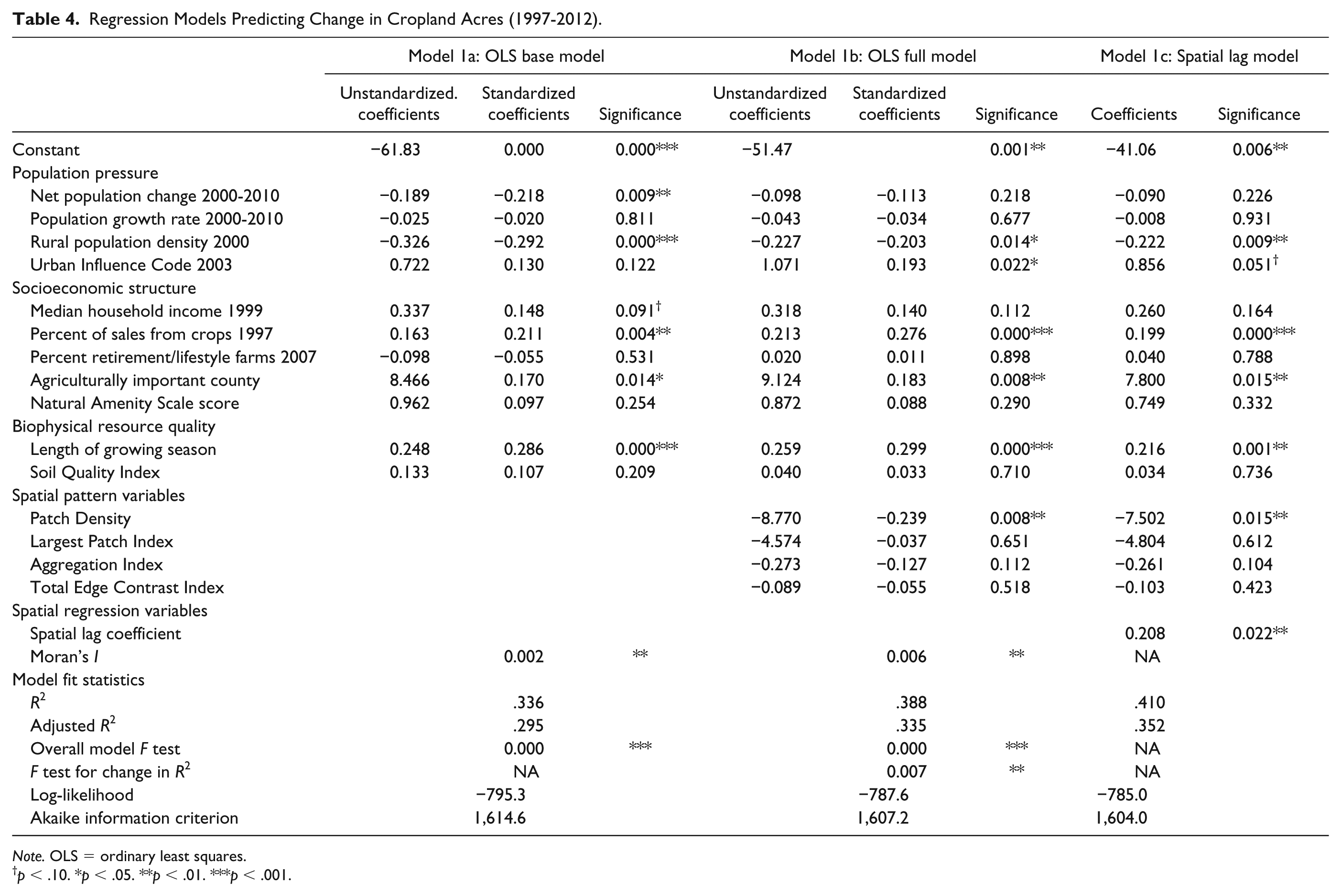
Coefficient estimates for similar OLS and spatial regression models to predict changes in cropland acres are shown in Table 4. A comparison of model fit statistics suggests that adding the spatial pattern variables in the full model (Table 4) improved model fit (adjusted R² rose from .295 to .335, and LL and AIC statistics declined). With respect to spatial pattern variables, the only predictor that was significant in the full OLS model was PD, which was negatively associated with cropland change. This suggests that the greater the number of developed patches in the non-urbanized landscape, the more rapid was the decline in cropland acres between 1997 and 2012.

Table 4.

Regression Models Predicting Change in Cropland Acres (1997-2012).

	Model 1a: OLS base model			Model 1b: OLS full model			Model 1c: Spatial lag model
	Unstandardized. coefficients	Standardized coefficients	Significance	Unstandardized coefficients	Standardized coefficients	Significance	Coefficients	Significance
Constant	−61.83	0.000	0.000***	−51.47		0.001**	−41.06	0.006**
Population pressure
Net population change 2000-2010	−0.189	−0.218	0.009**	−0.098	−0.113	0.218	−0.090	0.226
Population growth rate 2000-2010	−0.025	−0.020	0.811	−0.043	−0.034	0.677	−0.008	0.931
Rural population density 2000	−0.326	−0.292	0.000***	−0.227	−0.203	0.014*	−0.222	0.009**
Urban Influence Code 2003	0.722	0.130	0.122	1.071	0.193	0.022*	0.856	0.051^†
Socioeconomic structure
Median household income 1999	0.337	0.148	0.091^†	0.318	0.140	0.112	0.260	0.164
Percent of sales from crops 1997	0.163	0.211	0.004**	0.213	0.276	0.000***	0.199	0.000***
Percent retirement/lifestyle farms 2007	−0.098	−0.055	0.531	0.020	0.011	0.898	0.040	0.788
Agriculturally important county	8.466	0.170	0.014*	9.124	0.183	0.008**	7.800	0.015**
Natural Amenity Scale score	0.962	0.097	0.254	0.872	0.088	0.290	0.749	0.332
Biophysical resource quality
Length of growing season	0.248	0.286	0.000***	0.259	0.299	0.000***	0.216	0.001**
Soil Quality Index	0.133	0.107	0.209	0.040	0.033	0.710	0.034	0.736
Spatial pattern variables
Patch Density				−8.770	−0.239	0.008**	−7.502	0.015**
Largest Patch Index				−4.574	−0.037	0.651	−4.804	0.612
Aggregation Index				−0.273	−0.127	0.112	−0.261	0.104
Total Edge Contrast Index				−0.089	−0.055	0.518	−0.103	0.423
Spatial regression variables
Spatial lag coefficient							0.208	0.022**
Moran’s I		0.002	**		0.006	**	NA
Model fit statistics
R²		.336			.388		.410
Adjusted R²		.295			.335		.352
Overall model F test		0.000	***		0.000	***	NA
F test for change in R²		NA			0.007	**	NA
Log-likelihood		−795.3			−787.6		−785.0
Akaike information criterion		1,614.6			1,607.2		1,604.0

Note. OLS = ordinary least squares.

†

p < .10. *p < .05. **p < .01. ***p < .001.

The Moran’s I test for spatial autocorrelation for both base and full OLS models was highly significant, so we estimated spatial lag and spatial error models. Both generated models that were a better fit than the full OLS model, and both the spatial lag coefficient and lambda coefficients were significant. As the results of the two spatial models were nearly identical, we show only the spatial lag model coefficient estimates in Table 4. It is worth noting that the spatial lag coefficient was positive, again suggesting that trends in cropland acres in one county were positively associated with trends in their neighboring counties. The estimated coefficients and significance of all the other variables in the spatial lag model remained similar to those reported in the full OLS model.

With respect to trends in cropland change, rural population density in 2000 was again significantly and negatively associated with trends in cropland. In other words, increasing rural population density was linked to more rapid loss of cropland. In addition, more rural counties that were less proximate to major urban centers (those higher UICs) witnessed slower rates of cropland loss. Two socioeconomic structure variables were related to cropland trends. Counties which were more dependent on crop (as opposed to livestock) sales for their gross farm income and farmers in agriculturally important counties retained their cropland at higher rates. Length of growing season was again related to positive farm trends with lower rates of cropland loss in areas with more mild climates.

Explaining Farm Sales Change, 1997-2012

The final set of models focus on explaining trends in farm sales (Table 5). Once again, a model that included spatial pattern variables was significantly better at predicting changes in aggregate farm sales than the baseline model. Adjusted R² in the full model increased from .281 to .306 and F tests change in R² values were significant (p < .01). LL and AIC statistics also demonstrated an improvement in model performance for the full OLS model. Two spatial pattern variables were associated with farm sales trends. Initially, the measure of landscape heterogeneity (TECI) was significantly and negatively related to farm sales trends. This suggests that areas with development patterns that intersperse housing with agricultural fields are associated with a more negative rate of farm sales. Meanwhile, the AI was negatively (but weakly) related to changes in farm sales. This unexpected result suggests that more clustered forms of residential development were associated with slower increases in gross farm sales.

Table 5.

Regression Models Predicting Change in Farm Sales (1997-2012).

	Model 1a: OLS base model			Model 1b: OLS full model			Model 1c: Spatial lag model
	Unstandardized coefficients	Standardized coefficients	Significance	Unstandardized coefficients	Standardized coefficients	Significance	Coefficients	Significance
Constant	81.61		0.011*	108.95		0.002	74.93	0.018*
Population pressure
Net population change 2000-2010	−0.043	−0.023	0.788	0.212	0.111	0.232	0.155	0.332
Population growth rate 2000-2010	0.218	0.078	0.354	0.182	0.065	0.437	0.094	0.655
Rural population density 2000	−0.550	−0.224	0.005**	−0.383	−0.156	0.062^†	−0.384	0.037*
Urban Influence Code 2003	1.191	0.098	0.249	1.403	0.115	0.177	0.928	0.321
Socioeconomic structure
Median household income 1999	0.010	0.002	0.982	0.149	0.030	0.739	0.256	0.522
Percent of sales from crops 1997	0.203	0.120	0.099^†	0.335	0.198	0.012*	0.292	0.014*
Percent retirement/lifestyle farms 2007	−0.625	−0.159	0.074^†	−0.487	−0.124	0.166	−0.314	0.321
Agriculturally important county	7.713	0.071	0.309	12.184	0.112	0.111	11.739	0.086^†
Natural Amenity Scale score	−6.910	−0.318	0.000***	−6.927	−0.319	0.000***	−4.539	0.008**
Biophysical resource quality
Length of growing season	−0.063	−0.033	0.676	0.016	0.008	0.916	0.025	0.854
Soil Quality Index	−0.111	−0.041	0.633	−0.192	−0.071	0.428	−0.187	0.390
Spatial pattern variables
Patch Density				−2.595	−0.032	0.722	−3.370	0.607
Largest Patch Index				−1.041	−0.004	0.963	−0.586	0.977
Aggregation Index				−0.745	−0.159	0.053^†	−0.643	0.062^†
Total Edge Contrast Index				−0.813	−0.228	0.009**	−0.688	0.013*
Spatial regression variables
Spatial lag coefficient							0.369	0.000***
Moran’s I		0.002	**		0.006	**	NA
Model fit statistics
R²		.336			.388		.410
Adjusted R²		.295			.335		.352
Overall model F test		0.000	***		0.000	***	NA
F test for change in R²		NA			0.007	**	NA
Log-likelihood		−795.3			−787.6		−785.0
Akaike information criterion		1,614.6			1,607.2		1,604.0

Note. OLS = ordinary least squares.

†

p < .10. *p < .05. **p < .01. ***p < .001.

Results for the Moran’s I statistic test demonstrated strong and positive evidence of spatial auto-correlation in the regression residuals in both OLS models. Again, we estimated two spatial regression models to capture the effects of spatial processes. Both the spatial lag model and spatial error model produced improved adjusted R², LL ratios, and AIC statistics compared with the OLS full model. Spatial regression coefficients were also positive and significant in both the lag and error models, indicating positive spatial relationships in farm sales trends among neighboring counties in the region. Results for the spatial lag model (3c) are reported in Table 5. After controlling for spatial lag effects, the size and significance of the other independent variables remain largely unchanged.

With respect to trends in farm sales, the only significant demographic predictor was rural population density. Higher population density on rural privately developable land was associated with slower rates of growth in farm sales such that each one person increase in density per square mile was associated with a decrease of 0.4% in the predicted rate of farm sales change. Three indicators of socioeconomic structure were statistically significant. Areas with more sales from crops and farms in agriculturally important counties were more likely to see growth in farm sales over the study period. Meanwhile, counties with higher scores on the natural amenity index had lower rates of farm sales growth (net the effects of other variables in the model). Neither soil quality nor the length of growing season appeared to play a significant role in explaining variation in trends in farm sales in the region.

Conclusion

Traditionally, population growth is seen as presenting challenges for agriculture because it increases land consumption for non-agricultural purposes and reduces lands available for farming (Daniels, 1999; Jackson-Smith et al., 2006). In addition, population growth reduces farm viability due to the increased land prices, land use conflicts, and the loss of critical mass and infrastructure (Irwin & Bockstael, 2007). Pressure from residential development in low-density rural and exurban areas can contribute to declines in farm numbers, loss of working cropland, and diminishing agricultural economic activity (MacLaren et al., 2005). Alternatively, rising land values in urbanizing zones can lead to a shift toward production of higher value agricultural commodities (Thomas & Howell, 2003).

Many early studies of demographic impacts on agriculture focused on aggregate indicators of population growth and density at the county level (Smutny, 2002; Waisanen & Bliss, 2002). However, growth in the exurban and rural areas is likely to have more impact on farming than that which occurs within the boundaries of existing municipalities (Brown, Johnson, Loveland, & Theobald, 2005; Heimlich & Anderson, 2001; Theobald, 2001). This suggests that indicators of rural population pressure within the exurban zone may be more important than overall population growth within a county. Moreover, the spatial configuration of residential development should also affect the impacts on landscape fragmentation and the viability of farm operations (Radeloff, Hammer, & Stewart, 2005; Theobald et al., 1997).

Our findings provide support for the idea that growth pressure from settlement in rural and exurban areas is more closely associated with trends in agriculture than county-level population changes. The most consistent demographic predictor of farm changes in our models is the indicator of rural population density which was negatively related to cropland and farm sales trends and positively related to farm number trends. By contrast, indicators for net county population changes, the overall county growth rate, and indicators of urban proximity were not systematically related to farm trends in the IW between 1997 and 2012. The lack of a consistent relationship between overall county-level urbanization and farm trends may reflect the fact that intensive producers of high value crops and smaller hobby/lifestyle-oriented farms often thrive near urban areas (Jackson-Smith & Sharp, 2008). Conversely, because many farmers rely on off-farm income to sustain their households, living in areas where population growth is flat or in decline can be associated with diminishing local employment opportunities, and thus contribute to decline in the viability of farm households.

Taken as a whole, accounting for the spatial pattern of development in rural and exurban landscapes also improved our ability to explain variation in regional farm trends between 1997 and 2012. All four landscape metrics were related to at least one of the outcome measures. As expected, areas with a higher PD index score (or more distinct developed “patches” per square mile on the landscape) were associated with negative cropland trends, and areas with a greater degree of land use heterogeneity (TECI) were associated with lower rates of growth in farm sales. While statistically significant in two models, the two metrics designed to capture clustering/aggregation in residential development both produced unexpected results. Counties that had a greater proportion of development in a single contiguous area (as captured by the LPI) had slower growth in farm numbers. Meanwhile, counties with higher overall AI scores experienced more negative trends in farm sales. It would appear that clustering or aggregating new housing development may discourage hobby or recreational farming (which would explain the slower growth in farm numbers) but—net the effect of other variables in the model—has had little systematic impact on the ability to sustain or grow commercially viable farm operations. More research is needed to explain why consolidated patterns of rural housing development were negatively related trends in farm sales in this region.

Aside from the impacts of demographic pressure and spatial patterns of development, our findings suggest that the local socioeconomic opportunity structure has strong effects on agricultural trends. Areas with dense commercial farming sectors (agriculturally important counties) and greater reliance on crop (vs. livestock) income were all associated with more positive trends in cropland and farm sales (though more rapid losses in farm numbers). Retaining a critical mass of commercial farmers appears to be important to sustaining the economic viability of farming and slowing land use conversions. Higher median household income was associated with increases in farm numbers (e.g., more hobby farms), but had no relationship to trends in cropland or gross farm sales.

Interestingly, we found little evidence of a consistent relationship between farm trends and indicators of the growing New West recreational and service economy in the region, which confirms recent previous studies that suggest New West growth is not always in conflict with Old West economic activity (Jackson-Smith et al., 2006; Nelson, 2001). Meanwhile, counties with higher natural amenities and higher median household income (both indicators of “New West” counties) experienced more positive trends in farm numbers, more negative trends in farm sales, and no systematic relationship to cropland trends. Extensive livestock operations and hobby, lifestyle, or retirement farming can be both compatible with and even reflect the landscape aesthetic preferences of amenity migrants to many Western rural communities (Nelson, 2001; Winkler et al., 2007). While commercial scale agriculture may be in decline in many high amenity wealthy places in the IW, the growth in lifestyle farms and a preference for working open landscapes by amenity migrants leads these areas to be no more or less likely to be losing cropland than other places.

In addition to demonstrating the importance of including variables designed to capture spatial patterns of housing development, the results illustrate that conventional OLS models for analysis of county-level trends can have significant spatial correlation in regression residuals. The use of a spatial lag regression model helps address this potential problem by capturing how farm trends in one county are affected by their neighbors. Our results suggest that there are significant and positive associations in trends between neighboring counties. Future studies of the impacts of growth and development on agriculture should be attentive to these cross-border effects.

While our results are indicative of the statistical associations between county characteristics and farm trends, we were only to explain roughly 35% to 37% of the variation in the dependent variables. Inclusion of additional variables—such as measures of local land use policies; information about farm product marketing, processing, and transportation networks; and more nuanced and precise measure of low density rural housing development—might capture some of the unmeasured variance in our dependent variables. It would also be helpful to replicate the work using updated data from the Census of Agriculture and National Land Cover Dataset (released in late spring 2019), and in other regions that have different biophysical landscape attributes, farm types, and patterns of urban growth in exurban and rural areas. Changes in housing starts and population growth pressures across this region associated with the housing crisis after 2008 may well had long-term impacts that might be more prominent in agricultural trends that occurred after 2012.

Supplemental Material

Supplemental_File – Supplemental material for Impacts of Spatial Patterns of Rural and Exurban Residential Development on Agricultural Trends in the Intermountain West

Supplemental material, Supplemental_File for Impacts of Spatial Patterns of Rural and Exurban Residential Development on Agricultural Trends in the Intermountain West by Saleh Ahmed and Douglas Jackson-Smith in SAGE Open

Footnotes

Acknowledgements

The authors thank Dr. Molly Boeka Cannon for her help with spatial data analysis.

Declaration of Conflicting Interests

The author(s) declared no potential conflicts of interest with respect to the research, authorship, and/or publication of this article.

Funding

The author(s) disclosed receipt of the following financial support for the research, authorship, and/or publication of this article: The work was supported by the Utah Agricultural Experiment Station Project (UTA-01139).

ORCID iD

Saleh Ahmed

Supplemental Material

Supplemental material for this article is available online.

Author Biographies

Saleh Ahmed is an assistant professor in the School of Public Service at Boise State University. His research focuses on climate-society interactions, land use changes and rural livelihoods.

Douglas Jackson-Smith is a professor of Water Security and an assistant director of the School of Environment and Natural Resources at The Ohio State University. His research focuses on human dimensions of complex water systems and working landscapes.

References

Adelaja

Sullivan

Hailu

Y. G.

(2011). Endogenizing the planning horizon in urban fringe agriculture. Land Use Policy, 28, 66-75.

Alberti

(2005). The effects of urban patterns on ecosystem function. International Regional Science Review, 28, 168-192.

Anselin

(2002). Under the hood: Issues in the specification and interpretation of spatial regression models. Agricultural Economics, 27, 247-267.

Bartlett

P. F.

(1993). American dreams, rural realities: Family farms in crisis. Chapel Hill: The University of North Carolina Press.

Belyea

M. J.

Lobao

L. M.

(1990). Psychosocial consequences of agricultural transformation: The farm crisis and depression. Rural Sociology, 55, 58-75.

Berube

Singer

Wilson

J. H.

Frey

W. H.

(2006). Living Cities Census Series: Finding exurbia: America’s fast-growing communities at the metropolitan fringe. Washington, DC: Brookings Institute.

Bonanno

Constance

D. H.

(2006). Corporations and the state in the global era: The case of Seaboard Farms and Texas. Rural Sociology, 71, 59-84.

Brown

D. G.

Johnson

K. M.

Loveland

T. R.

Theobald

D. M.

(2005). Rural land-use trends in the coterminous United States, 1950-2000. Ecological Applications, 15, 1851-1863.

Cadieux

K. V.

Hurley

P. T.

(2011). Amenity migration, exurbia, and emerging rural landscapes: Global natural amenity as place and as process. Geoforum, 76, 297-302.

10.

Carruthers

J. I.

Ulfarsson

G. F.

(2008). Does “smart growth” matter to public finance? Urban Studies, 45, 1791-1823.

11.

Clark

McChesney

Munroe

D. K.

Irwin

E. G.

(2009). Spatial characteristics of exurban settlement pattern in the United States. Landscape and Urban Planning, 90, 178-188.

12.

Cochrane

W. W.

(1993). The development of American agriculture: A historical analysis. Minneapolis: University of Minnesota Press.

13.

Compas

(2007). Measuring exurban change in the American West: A case study in Gallatin County, Montana, 1973–2004. Landscape and Urban Planning, 82, 56-65.

14.

Daniels

(1999). When city and country collide: Managing growth in the metropolitan fringe. Washington, DC: Island Press.

15.

Deng

J. S.

Wang

Hong

J. G.

(2009). Spatio-temporal dynamics and evolution of land use change and landscape pattern in response to rapid urbanization. Landscape and Urban Planning, 92, 187-198.

16.

DiBari

J. N.

(2007). Evaluation of five landscape-level metrics for measuring the effects of urbanization on landscape structure: The case of Tucson, Arizona, USA. Landscape and Urban Planning, 79, 308-313.

17.

Dirimanova

(2006). Land fragmentation in Bulgaria: An obstacle for land market development. Annals of the Polish Association of Agricultural and Agribusiness Economists, 8(6), 37-42.

18.

Fagan

W. F.

Meir

Carroll

S. S.

(2001). The ecology of urban landscapes: Modeling housing starts as a density-dependent colonization process. Landscape Ecology, 16, 33-39.

19.

Ferrari

Pezzi

Diani

Corazza

(2008). Evaluating landscape quality with vegetation naturalness maps: An index and some references. Applied Vegetation Science, 11, 243-250.

20.

Foltz

Zeuli

(2005). The role of community and farm characteristics in farm input purchasing patterns. Review of Agricultural Economics, 27, 508-525.

21.

GeoDa Center. (2014). GeoDa. Available from http://geodacenter.asu.edu/

22.

Gill

Klepeis

Chisholm

(2010). Stewardship among lifestyle oriented rural landowners. Journal of Environmental Planning and Management, 53, 317-334.

23.

Goldschmidt

(1978). As you sow: Three studies in the social consequences of agribusiness. Montclair, NJ: Allanheld, Osmun.

24.

Gollehon

Quinby

(2000). Irrigation in the American west: Area, water and economic activity. Water Resources Development, 16, 187-195.

25.

Gude

P. H.

Hansen

A. J.

Rasker

Maxwell

(2006). Rates and drivers of rural residential development in the Greater Yellowstone. Landscape and Urban Planning, 77, 131-151.

26.

Gustafson

E. J.

(1998). Quantifying landscape spatial pattern: What is the state of the art? Ecosystems, 1, 143-156.

27.

Hargiss

C. D.

Bissonette

J. A.

David

J. L.

(1998). The behavior of landscape metrics commonly used in the study of habitat fragmentation. Landscape Ecology, 13, 167-186.

28.

H. S.

DeZonia

B. E.

Mladenoff

D. J.

(2000). An Aggregation Index (AI) to quantify spatial patterns of landscapes. Landscape Ecology, 15, 591-601.

29.

Headwaters Economics. (2012). West is best: Protected lands promote jobs and higher incomes—How public lands in the West create a competitive economic advantage. Retrieved from http://headwaterseconomics.org/land/west-is-best-value-of-public-lands

30.

Heimlich

R. E.

Anderson

W. D.

(2001). Development at the urban fringe and beyond (AER-803). Washington, DC: U.S. Department of Agriculture Economic Research Service.

31.

Heinman

M. K.

(1989). Production confronts consumption: Landscape perception and social conflict in the Hudson Valley. Environment and Planning D: Society and Space, 7, 165-178.

32.

Hersperger

A. M.

(2006). Spatial adjacencies and interactions: Neighborhood mosaics for landscape ecological planning. Landscape and Urban Planning, 77, 227-239.

33.

Hines

J. D.

(2010). Rural gentrification as permanent tourism: The creation of the “New” West Archipelago as postindustrial cultural space. Environment and Planning D: Society and Space, 28, 509-525.

34.

Hoppe

R. A.

MacDonald

J. M.

(2013, April). Updating the ERS farm typology (EIB-110). Washington, DC: U.S. Department of Agriculture Economic Research Service.

35.

Hung

P. V.

MacAulay

T. G.

Marsh

S. P.

(2007). The economics of land fragmentation in the north of Vietnam. The Australian Journal of Agricultural and Resource Economics, 51, 195-211.

36.

Irwin

E. G.

Bockstael

N. E.

(2007). The evolution of urban sprawl: Evidence of spatial heterogeneity and increasing land fragmentation. Proceedings of the National Academy of Sciences, 104, 20672-20677.

37.

Irwin

E. G.

Cho

H. J.

Bockstael

N. E.

(2007). Measuring the amount and pattern of land development in nonurban areas. Review of Agricultural Economics, 29, 494-501.

38.

Jackson-Smith

(1999). Understanding the microdynamics of farm structural change: Entry, exit, and restructuring among Wisconsin family farmers in the 1980s. Rural Sociology, 64, 66-91.

39.

Jackson-Smith

(2003). Transforming rural America: The challenges of land use change in the twenty-first century. In Brown

D. L.

Swanson

L. E.

(Eds.), Challenges for rural America in the twenty-first century (pp. 305-316). University Park: The Pennsylvania State University Press.

40.

Jackson-Smith

(2004). The social aspects of agriculture. In Manfredo

M. J.

Vaske

J. J.

Field

D. R.

Brown

P. J.

Bruyere

B. L.

(Eds.), Society and natural resources: A summary of knowledge (pp. 159-174). Jefferson City, MO: Modern Litho.

41.

Jackson-Smith

Gillespie

G. W.

Jr. (2005). Impacts of farm structural change on farmer’s social ties. Society and Natural Resources, 18(3), 1-26.

42.

Jackson-Smith

Jensen

E. E.

(2009). Agricultural importance versus farm dependence: A new typology. Rural Sociology, 74, 37-55.

43.

Jackson-Smith

Jensen

E. E.

Jennings

(2006). Changing land use in the rural Intermountain West. In Kandel

W. A.

Brown

D. L.

(Eds.), Population change and rural society. Dordrecht, The Netherlands: Springer.

44.

Jackson-Smith

Sharp

(2008). Farming in the urban shadow: Supporting agriculture at the rural-urban interface. Rural Realities, 2(4), 1-12.

45.

Keske

C. M. H.

Bixler

R. P.

Bastian

C. T.

Cross

J. E.

(2017). Are population and land use changes perceived as threats to sense of place in the New West? A multilevel modeling approach. Rural Sociology, 82, 263-290.

46.

Krannich

Luloff

A. E.

Field

D. R.

(2011). People, places and landscapes: Social change in high amenity rural areas. Dordrecht, The Netherlands: Springer.

47.

Lobao

Meyer

(2001). The great agricultural transition: Crisis, change, and social consequences of twentieth century US farming. Annual Review of Sociology, 27, 103-124.

48.

Logan

(2012). Making a place for space: Spatial thinking in social science. Annual Review of Sociology, 38, 1-20.

49.

Low

S. A.

Adalja

Beaulieu

Key

Martinez

Melton

. . . Jablonski

B. B. R.

(2015). Trends in U.S. local and regional food systems (AP-068). U.S. Department of Agriculture Economic Research Service. Retrieved from https://www.ers.usda.gov/webdocs/publications/42805/51173_ap068.pdf

50.

Luck

(2002). A gradient analysis of urban landscape pattern: A case study from the Phoenix metropolitan region, Arizona, USA. Landscape Ecology, 17, 327-339.

51.

MacLaren

Kimball

Holmes

Eisenbeis

(2005). Too many homes on the range: The impact of rural sprawl on ranching and habitat. Retrieved from www.friends.org/sites/friends.org/files/reports/too_many_homes.pdf

52.

McGarigal

Cushman

S. A.

Ene

(2013). FRAGSTATS: Spatial pattern analysis program for categorical maps (Version 4.0). Retrieved from www.umass.edu/landeco/research/fragstats/fragstats.html

53.

McGranahan

D. A.

(1999). Natural Amenities drive rural population change (No. 781). Washington, DC: Food and Rural Economics Division, Economic Research Service, U.S. Department of Agriculture. Retrieved from https://www.ers.usda.gov/webdocs/publications/41047/13201_aer781.pdf?v=42061

54.

McKinney

Harmon

(2002). Land use planning and growth management in the American West. Montana Policy Review, 9, 1-6.

55.

McNabb

W. H.

Avers

P. E.

(1994). Ecological subregions of the United States: Section descriptions (Administrative Publication WO-WSA-5). Washington, DC: U.S. Department of Agriculture. Retrieved from http://www.fs.fed.us/land/pubs/ecoregions/

56.

Multi-Resolution Land Characteristics Consortium. (2013). NLCD Data 2011. Available from http://www.mrlc.gov/

57.

Nelson

P. B.

(2001). Rural restructuring in the American West: Land use, family and class discourses. Journal of Rural Studies, 17, 395-407.

58.

Otterstrom

S. M.

Shumway

J. M.

(2003). Deserts and oases: The continuing concentration of population in the American Mountain West. Journal of Rural Studies, 19, 445-462.

59.

Palmer

J. F.

(2004). Using spatial metrics to predict scenic perception in a changing landscape: Dennis, Massachusetts. Landscape and Urban Planning, 69, 201-218.

60.

Petrzelka

Malin

S. A.

(2013). The elephant in the room: Absentee landowners and conservation management. Land Use Policy, 30, 157-166.

61.

Potter

Lobely

(1992). Aging and succession on family farms—The impact on decision-making and land-use. Sociologia Ruralis, 32, 317-334.

62.

Power

T. M.

Barrett

R. N.

(2011). Post-cowboy economics: Pay and prosperity in the new American West. Washington, DC: Island Press.

63.

Primdahl

(2014). Agricultural landscape sustainability under pressure: Policy developments and landscape change. Landscape Research, 39, 123-140.

64.

Radeloff

V. C.

Hammer

R. B.

Stewart

S. I.

(2005). Rural and suburban sprawl in the U.S. Midwest from 1940 to 2000 and its relation to forest fragmentation. Conservation Biology, 19, 793-805.

65.

Sinclair

(1967). Von Thünen and urban sprawl. Annals of the Association of American Geographers, 57, 72-87.

66.

Smutny

(2002). Patterns of growth and change: Depicting the impacts of restructuring in Idaho. The Professional Geographer, 54, 438-453.

67.

Theobald

D. M.

(2001). Land-use dynamics beyond the American urban fringe. Geographical Review, 91, 544-565.

68.

Theobald

D. M.

Gosnell

Riebsame

W. E.

(1996). Land use and landscape change in the Colorado Mountains, II: A case study of the East River Valley. Mountain Research and Development, 16, 407-418.

69.

Theobald

D. M.

Miller

J. R.

Hobbs

N. T.

(1997). Estimating the cumulative effects of development on wildlife habitat. Landscape and Urban Planning, 39, 25-36.

70.

Thomas

J. K.

Howell

F. M.

(2003). Metropolitan proximity and U.S. agricultural productivity, 1978-1997. Rural Sociology, 68, 366-386.

71.

Travis

W. R.

(2007). New geographies of the American West: Land use and the changing patterns of place. Washington, DC: Island Press.

72.

U.S. Bureau of Census. (2014). Population census, 2000 and 2010. Washington, DC. Available from www.census.gov

73.

U.S. Department of Agriculture-Economic Research Service. (2014). Urban influence codes. Washington, DC: Author. Retrieved from https://www.ers.usda.gov/data-products/urban-influence-codes.aspx

74.

U.S. Department of Agriculture-National Agricultural Statistics Service. (2012). U.S. Department of Agriculture Census of Agriculture 2012. Washington, DC. Retrieved from http://www.agcensus.usda.gov/Publications/2012/

75.

von Thünen

J. H

. (1966). Isolated state (English ed.). Oxford, UK: Pergamon Press.

76.

Waisanen

P. J.

Bliss

N. B.

(2002). Changes in population and agricultural land in coterminous United States counties, 1790 to 1997. Global Biogeochemical Cycles, 16, 1137.

77.

Walker

R. T.

Solecki

W. D.

(1999). Managing land use and land cover change: The New Jersey Pinelands Biosphere Reserve. Annals of the Association of American Geographers, 89, 219-236.

78.

Weng

Y. C.

(2007). Spatiotemporal changes of landscape pattern in response to urbanization. Landscape and Urban Planning, 81, 341-353.

79.

Winkler

Field

D. R.

Luloff

A. E.

Krannich

R. S.

Williams

(2007). Social landscapes of the Inter-Mountain West: A comparison of “Old West” and “New West” communities. Rural Sociology, 72, 478-501.

Supplementary Material

Please find the following supplemental material available below.

For Open Access articles published under a Creative Commons License, all supplemental material carries the same license as the article it is associated with.

For non-Open Access articles published, all supplemental material carries a non-exclusive license, and permission requests for re-use of supplemental material or any part of supplemental material shall be sent directly to the copyright owner as specified in the copyright notice associated with the article.

0.00 MB

0.30 MB