Zero-Coupon and Forward Yield Curves for Government of Ghana Bonds

Abstract

This article seeks to provide a framework for modeling daily zero-coupon yield curve for Government of Ghana bonds based on secondary market daily trades. It also proposes method for modeling the forward yield curve. The current practice in Ghana is to produce yield curve for Government of Ghana bonds based on primary market weekly auctions. This article demonstrates the extraction and fitting of secondary market daily yield curves for Government of Ghana bonds, using bootstrapping and piecewise cubic hermite interpolation. The article also compares the piecewise cubic hermite method with the piecewise cubic spline method, the Nelson–Siegel–Svensson model, and the penalized smoothing spline method. Data used are the daily bond price data from the Ghana Fixed Income Market, accessible at the Central Securities Depository of Ghana. The results show yield curves that reflect the actual daily yield movements in the secondary bond market of Ghana. The results also show that the piecewise cubic hermite method fits the zero-coupon yield curve better than the other methods as far as the Ghanaian bond market is concerned. For the forward curves, we recommend that either or both of the piecewise cubic hermite method and the Nelson–Siegel–Svensson method could be used by the market participants.

Introduction

The bond market of every country does not only help the government to raise funds to finance its budget deficits and the corporate bodies to raise debt capitals; but it also has a direct impact on the extent to which other aspects of the entire financial market can develop. In addition, the bond market provides yield curves which contain important information for conducting monetary policy functions. Over the years, the Government of Ghana (GoG) has taken several steps to develop the credit sector of the financial market of Ghana. During the postindependence period (after 1957), the GoG implemented policies to regulate the financial sector with the aim of achieving rapid industrialization and economic development. There were interest rate controls and credit ceilings to ensure that cheap credit was made available to the government to develop sectors considered very important. Unfortunately, rising inflation and nonperforming loans in the banking sector subsequently led to the backsliding of the economy. In 1983 the GoG launched the Economic Recovery Program (ERP) under the guidance of the World Bank and the International Monetary Fund (IMF). This led to many financial sector reforms; including the liberalization of asset prices and interest rates. Interest rates were made to be in line with market conditions (Antwi-Asare & Addison, 2000). Auction of GoG treasury bills and Bank of Ghana (BoG) bills were introduced in the late 1980s to take care of excess liquidity in the economy and to provide more avenues for investment. The Financial Sector Structural Adjustment Program (FINSAP) was also established to ensure effective mobilization of domestic savings and efficient allocation of loanable funds. Nonperforming loans of the banks were replaced by FINSAP bonds by the BoG. To encourage secondary market trading, the Ghana Stock Exchange (GSE) was established in 1989 and it started operation in 1990. Few bonds, including the GSE Commemoration Registered Stock were listed on the stock exchange. Money market instruments however, were traded in the secondary market over the counter.

The GoG did not relent afterward; subsequent efforts were made to achieve the needed developments in the domestic bond market. In the early 2000s, the National Bond Market Committee (NBMC) was formed by the GoG to make recommendations for the development of the bond market. Based on the committee’s recommendations, the BoG established the Central Securities Depository (CSD) in 2004; while the GSE also established the GSE Securities Depository (GSD) in 2008. The CSD and GSD were later merged into a single depository, named the CSD and took effect in January 2014. In 2015, the Ghana Fixed Income Market (GFIM) was established under the auspices of the GSE to facilitate the secondary market trading of all fixed income securities in Ghana. During the same year 2015, GFIM adopted the Bloomberg E-Bond trading and market surveillance system to ensure credible and globally competitive secondary debt market in Ghana. The Ghanaian bond market has clearly undergone some level of developments over the years.

Over the very recent years (per available data), the entire bond market capitalization (both government and nongovernment) increased by 217.95% from 10,348.68 million Ghana cedis (US$3,943.97 million) as at the end of 2011, to 32,903.91 million Ghana cedis (US$12,539.96 million) as at the end of 2015, which means an average annual growth rate of 33.53%. (The exchange rate was 1.4576 Ghana cedis to 1 US dollar in 2011 and 3.7902 Ghana cedis to 1 US dollar in 2015; we apply an average of 2.6239 Ghana cedis to 1 US dollar for these analyses.) The government bond market capitalization also increased by 218.95% from 9,117.63 million Ghana cedis (US$3,474.81 million) as at the end of 2011, to 29,080.90 million Ghana cedis (US$11,082.98 million) as at the end of 2015, also resulting in an average annual growth rate of 33.64% (Figure 1). These figures or numbers point to the fact that the Ghanaian bond market is growing (even though it is heavily dominated by the government bonds).

Figure 1.

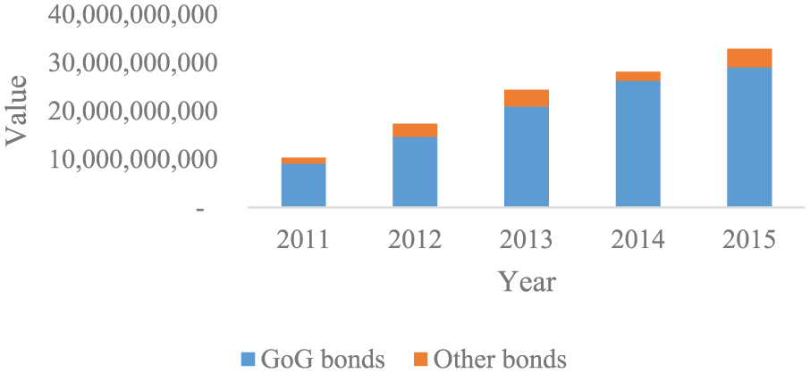
Bond market capitalization.

However, one important ingredient missing in the bond market of Ghana is the yield curve. There are no zero-coupon and forward yield curves in the bond market of Ghana. Meanwhile, according to the International Organization of Securities Commissions (IOSCO), one of the key requirements for the development of the bond market is the government yield curve. The government yield curve serves as a benchmark for pricing corporate bonds and other financial assets and derivatives. The yield curve currently used in Ghana is a primary market auction yield curve which is produced by the BoG. The Ghanaian bond market needs a secondary market benchmark zero-coupon yield curve for pricing corporate bonds and other securities. The market also needs forward yield curve for pricing forward contracts and other derivatives. There are important reasons why the Ghanaian bond market urgently needs these benchmark yield curves.

First, these curves could enhance the development of the entire financial market of Ghana. As stated earlier, they would be used for pricing corporate bonds and other financial instruments and derivatives. Presently, the corporate bond market of Ghana is not active; and there are no active markets for derivatives and asset-backed securities. As at the end of 2017, for instance, only seven companies had their bonds trading on the GFIM. According to IOSCO (2011), one of the key impediments to the development of the corporate bond market is the nonexistence of benchmark yield curve. In the absence of the benchmark yield curve, pricing of corporate bonds is constrained (IOSCO, 2011).

Second, the yield curve would reveal, on timely basis, the expectations and assumptions of market participants, concerning the financial market and the macroeconomy of the country (Diebold, Rudebusch, & Aruoba, 2006). Financial market participants in Ghana need to know the level of, and the movements in the secondary market bond yields for the purpose of trade decision making. The BoG also needs to know the changes in the yield curve to monitor the market’s sentiments about the macro-economy.

The purpose of this article is to model the secondary market zero-coupon and forward yield curves for the GoG bonds using various methods of yield curve modeling. The article seeks to compare the piecewise cubic hermite method with other methods such as the piecewise cubic spline method (with not-a-knot end conditions), the penalized smoothing spline method, and the Nelson–Siegel–Svensson (NSS) method. (The article uses the Variable Roughness Penalty or VRP approach to the penalized smoothing spline. We therefore use the terms penalized smoothing spline and VRP interchangeably in the article.) Virtually, the article is comparing the spline-based methods of yield curve modeling with the parametric methods, using data from an illiquid African bond market (Ghana).

The remaining of the article is organized as follows. Section 2 reviews relevant literature; Section 3 discusses the methodology and data; Section 4 discusses the results; and Section 5 provides conclusion, recommendations and theoretical implications.

Literature Review

Empirical Review

There are two main categories of yield curve fitting methods. These are the parametric methods and the spline-based methods. Parametric methods involve the specification of a single-piece function defined over the entire maturity range. Model parameters are determined through minimization of squared deviation of theoretical prices from observed prices. A popular example of the parametric models is the Nelson–Siegel model (Nelson & Siegel, 1987). This model is extended by Svensson (1994), resulting in what is sometimes referred to as Nelson-Siegel-Svensson (NSS) model. According to James and Webber (2000), even though these parametric methods capture the overall shape of the yield curve fairly well, they are recommended when good accuracy is not a requirement. Considering the illiquidity of the Ghanaian bond market and data constraints, we prefer a method that would enhance the accuracy of the yield curve as much as possible.

A spline is a piecewise polynomial function, consisting of several individual polynomial segments that are joined together at knot points. Instead of using a single functional form over the entire maturity range, the spline-based methods employ the use of piecewise polynomials to fit the yield curve over the maturity range. To ensure continuity and smoothness, the splines join at the knot points and must be differentiable at the knot points. There is a wide range of spline-based methods of fitting the yield curve, varying in complexity. Examples include Cubic Spline (Waggoner, 1997); B-Spline (Steeley, 1991); Smoothing Spline (Fisher, Nychka, & Zervos, 1995) and Penalized Spline (Jarrow, Ruppert, & Yu, 2004). Choudhry (2004) thinks that although the spline approach can lead to unrealistic shapes for the forward curve (due to its divergence at the long end), it is an accessible method and one that gives reasonable accuracy for the zero-coupon yield curve. We therefore recommend a spline-based method for modeling the zero-coupon yield curve for the Ghanaian bond market. Our specific choice of spline-based method is mentioned elsewhere later in this section.

The Bank for International Settlements (BIS) has recommended that central banks adopt methods for estimating zero-coupon yields. After a meeting held in 1996 concerning the estimation of zero-coupon yield, many central banks have been reporting their zero-coupon yield estimates, as well as the methods of estimation, to the BIS (2005). Table 1 shows the methods used by some central banks to estimate zero-coupon yields. Most of these central banks use either a variation of the NSS model or a form of spline-based methods.

Table 1.

Yield Estimation Methods by Some Central Banks.

Central bank	Method of estimation
Belgium	Nelson–Siegel or Nelson–Siegel–Svensson
Canada	Merrill Lynch Exponential Spline
China	Hermite Interpolation Method
Finland	Nelson–Siegel
France	Nelson–Siegel or Nelson–Siegel–Svensson
Germany	Nelson–Siegel–Svensson
Italy	Nelson–Siegel
Japan	Smoothing Spline Interpolation
Norway	Nelson–Siegel–Svensson
Spain	Nelson–Siegel or Nelson–Siegel–Svensson
Sweden	Smoothing Splines and Nelson–Siegel–Svensson
Switzerland	Nelson–Siegel–Svensson
United Kingdom	Variable Roughness Penalty
United States	Quasi-Cubic Hermite Spline

Source. Adapted from Bank for International Settlements (BIS; 2005).

Many African central banks (including the BoG) are yet to adopt a method of estimating the zero-coupon yields. According to a survey by the African Financial Market Initiative (AFMI; 2016), while some central banks in Africa do not have any yield curve at all (e.g., Burundi), others solely rely on primary market auction yields to produce the yield curve (e.g., Ghana). Yet still, others also use indicative yields (e.g., Malawi). Only very few African countries currently produce yield curves based on secondary market trades (e.g., South Africa). Nevertheless, there are some researches going on to propose yield curve modeling methods for the African central banks and bond markets.

As far as Africa is concerned, South Africa does not only have the most developed bond market (Adelegan & Radzewicz-Bak, 2009; Mu, Phelpsb, & Stotsky, 2013), but it is also where yield curve estimation is most advanced (AFMI, 2016). In 2003, the then Bond Exchange of South Africa adopted a method of estimating zero-coupon yield curves. These curves served the purpose of providing benchmarking and valuation tools for the South African bond market. Subsequently, the Johannesburg Stock Exchange (JSE) considered these curves to be outdated; and a new set of curves were generated using a different methodology referred to as Monotone Preserving Interpolation. This new method involves the use of bootstrapping and shape preserving interpolation to fit the yield curve (JSE, 2012; Preez & Maré, 2013). The method is based on the Monotone Convex method by Hagan and West (2006, 2008), who emphasize the importance of shape preservation in yield curve modeling. The JSE zero-coupon yield curves now comprise three different daily yield curves: one for the nominal bond market, one for the nominal swaps market, and one for the inflation-linked bond market. Yield estimation in South Africa is very active because the South African bond market produces the volume of trade and data needed for the daily curves, as far as benchmarking is concerned. However, Ghana cannot boast of such volume of trade and data availability. While the input data for South African daily yield curves are from liquid bond and swap trades, Ghana can only rely on limited data from its illiquid (but developing) bond market. We therefore would not strictly adopt the Monotone Preserving method used by South Africa; but adopt a variation which could preserve shape.

In Kenya, according to Muthoni, Onyango, and Ongati (2015), there is currently no agreed-upon method used to construct yield curves. The existing practice is that financial companies use in-house methods to construct yield curves for pricing and other decision-making purposes. This is because some market participants think the yield curve produced by Nairobi Securities Exchange (NSE) has some limitations. They claim the prices and yields of secondary market trades reported at the NSE do not reflect the market (Cannon Asset Managers [CAM], 2011). With data supplied by the Central Bank of Kenya, CAM (2011) proposes a yield curve to the NSE using Logarithmic Linear Interpolation. However, because all variations of linear interpolation result in curves which are not differentiable, we do not recommend the use of any form of linear interpolation for modeling yield curve for Ghana.

In Nigeria, the Central Bank of Nigeria is at the forefront of providing the necessary prerequisites to develop the Nigerian bond market. One good step in this regard is the initiative to commission a project to fit the Nigerian government yield curve (Sholarin, 2014). Currently, Nigeria uses Financial Market Dealers Quotation (FMDQ) Methodology to fit the market yield curve. Sholarin (2014) seeks to use bootstrapping and piecewise cubic spline method to model the Nigerian zero-coupon yield curve for the Central Bank of Nigeria. However, we do not recommend this piecewise cubic spline method for Ghana, due to a reason mentioned shortly under this section.

In Ghana the yield-related works done for Ghana so far include Dzigbede and Ofori (2004) and Churchill and Mensah (2014). Both papers seek to estimate real interest rates using yield curve. Logubayom, Nasiru, and Luguterah (2013) also seek to forecast the weekly bill rates in the primary market. Ida and Albert (2014) investigate the relationship between the primary market bill rates, inflation rates and exchange rates in Ghana. Iyke (2017) analyzes the comovements of the BoG monetary policy rates and the bill rates in Ghana. The yields used in all these works are primary market yields, as the only form of yield curve presently in Ghana is the primary market yield curve. It is therefore not surprising that in a BoG working paper, Dzigbede and Ofori (2004) recommend that a research should be focused on building a framework to model the yield curve for the GoG debt securities. And that’s what this article seeks to do.

Due to illiquidity and data constraints in the Ghanaian bond market, resulting in wide gaps in-between data points, we need to use an interpolation method which can preserve shape and is differentiable as well. The method must be smoother than linear interpolation, but less smooth than piecewise cubic spline interpolation. This method is the piecewise cubic hermite interpolation. It is also a spline-based method based on cubic polynomials; but the estimation process is quite different from the traditional piecewise cubic spline method. (For the avoidance of confusion, and for the remaining of this article, we would use “Cubic Spline” or “Spline” to mean the piecewise cubic spline [with not-a-knot end conditions]; and use “Cubic Hermite” or “Hermite” to mean the piecewise cubic hermite.) The purpose of this work is to propose a framework for modeling secondary market zero-coupon and forward yield curves for GoG bonds. Specifically, this work compares the use of the Hermite method with other methods such as the Cubic Spline method, the penalized smoothing spline method, and the NSS method. The article seeks to make the following contributions:

1. This would be the first work, to the best of our knowledge, to model both the zero-coupon and forward yield curves for the Ghanaian bond market.

2. The article compares the Hermite method with other spline-based methods (Cubic Spline and penalized smoothing spline) for modeling secondary market daily yield curves for an illiquid African bond market.

3. This work empirically shows that for illiquid and inactive secondary bond markets, the Cubic Hermite method could work better than the Cubic Spline method (with not-a-knot end conditions).

4. The article also in general compares the spline-based methods with parametric methods of yield curve modeling based on data from an illiquid African bond market.

5. This work serves as a step toward the development of a database of secondary market daily yield curves for GoG bonds. This would provide a source where daily yield curves could be accessed by researchers, financial analysts, policy makers, investors, and other market participants.

Theoretical Review

The shape of the yield curve provides useful information in the bond market. There are some main theories that seek to explain the shape of the yield curve. One group of these theories interpret the shape of the yield curve in terms of investors’ expectations. These are collectively known as the expectations theories. The first of these theories is the pure expectations theory or the unbiased expectations theory. This theory asserts that the forward yields are unbiased predictors of future spot yields (zero-coupon yields). In other words, forward yields are what investors expect spot yields (or zero-coupon yields) to be in future. The broadest interpretation of this theory is that bonds of any maturity are perfect substitutes for one another (Chartered Financial Analyst [CFA] Institute, 2018). Thus, instead of investing in a 2-year bond at once, one could choose to first invest in a 1-year bond; and at maturity, reinvest the proceeds in another 1-year bond (making a total of 2-year horizon, and yielding the same total returns as if it is an investment in a 2-year bond). In addition, according to the pure expectations theory, the slope of the yield curve reflects only investors’ expectations for future short-term interest rates. Thus, an upward-sloping yield curve means investors expect the future short-term yields to increase; and a downward-sloping yield curve means investors expect future short-term yields to decrease. A flat yield curve therefore means investors expect short-term yields to remain constant in future. The pure expectations theory does not make any reference to risk premium as a factor affecting the shape of the yield curve. The second of the expectations theories is the local expectations theory. The local expectations theory does not explicitly assert that bonds of any maturity are perfect substitutes for one another; but rather, it asserts that the expected return for every bond over short time periods is the risk-free rate. While the pure expectations theory requires no risk premium along the entire maturity spectrum of the yield curve, the local expectations theory only requires existence of risk free at the very short end of the yield curve (no risk-free requirement is made for the longer ends of the yield curve). Therefore, unlike the pure expectations theory, the local expectations theory is applicable to both risk-free and risky bonds (CFA Institute, 2018).

The second main theory of yield curve is an “off-shoot” of the expectations theory. It is the liquidity preference theory or the liquidity premium theory. This theory views bonds of different maturities as substitutes (but not perfect substitutes). It is therefore sometimes referred to as the biased expectations theory. It is based on the premise that investors prefer liquid (short-term) bonds to long-term bonds because the former are free of inflation and interest rate risks. Investors would prefer to pay premium to buy short-term assets rather than to buy long-term assets. Thus, investors would have to be paid liquidity risk premium for holding long-term bonds (in lieu of short-term bonds). Because of this term premium, per the theory, long-term bond yields tend to be higher than short-term yields. The liquidity preference theory therefore predicts upward-sloping yield curves. The theory also implies that the forward yields do not only reflect expectations about future spot (zero-coupon) yields but they also reflect expectations about risk premiums for holding long-term bonds. Accordingly, the theory implies that forward yields reflect higher yields demanded by investors for buying long-term bonds.

The third theory is the market segmentation theory or the segmented market theory. This theory asserts that markets for different maturities of bonds are completely segmented. This implies that bonds of different maturities are not substitutes for one another. According to the theory, the shape of the yield curve is not a reflection of expected future spot rates; and neither does it reflect liquidity risk premiums. Instead, the theory asserts that the shape of the yield curve is a reflection of the demand and supply activities of the segmented market participants with respect to the specific maturities of interest. The yields of bonds of particular maturities are determined by the demand for, and the supply of such bonds; and without regard to the yields of other bonds of different maturities. Hence, the yield curve movement at one point is independent of the yields pertaining to the other segments of the yield curve. As an example, short-term maturity bonds may be preferred by mutual funds while long-term maturity bonds may be preferred by life insurance companies. Other investors may also prefer bonds of other maturities. If the demand for short-term maturity bonds (by mutual funds) exceed the supply of these bonds, their prices would rise and their yields would fall, leading to a decrease at the short end of the yield curve. Conversely, if the supply of the short-term securities exceeds their demand (by the mutual funds), the prices would fall, and the yields would rise, leading to an increase at the short end of the yield curve. Same demand and supply interaction applies to the long end (and other segments) of the yield curve.

The fourth theory is the preferred habitat theory which is an off-shoot or an extension of the segmented market theory. The preferred habitat theory also recognizes the fact that market participants have preferences for particular maturities (or habitats). That is, some investors prefer short-term maturity bonds, others prefer long-term maturity bonds, while there are others who also prefer medium-term maturity bonds. However this theory does not assert that yields at different maturities are determined independently of each other. The theory posits that investors may be willing to move out of their preferred maturity segments (or habitats) to buy bonds of other maturities if those bonds provide higher returns or yields enough to benefit the investors. Similarly, for investors to buy bonds outside their preferred maturities (i.e., outside the investors’ preferred investment horizons), those bonds must provide higher yields (or premiums) enough to compensate the investors. Thus, the shape of the yield curve is not only a reflection of the demand and supply activities of the investors; but more importantly, it is a reflection of the premiums required by investors before investing at curve segments outside their preferred investment horizons. For example, a mutual fund may require some risk premium before buying bonds outside the preferred investment horizon (of short term). Just like the segmented theory, the preferred habitat theory is consistent with any shape of the yield curve. However, as it is assumed that more investors prefer short-term habitats, this theory explains predominance of upward-sloping yield curves. Somehow consistent with the liquidity preference theory, the preferred habitant theory posits that for short-term maturity bond investor to buy long-term bonds, the long-term bonds must provide higher premiums.

Data and Methodology

We do the modeling in the following stages: (a) obtaining the daily bond data from the GFIM, (b) filtration of the bond data, (c) extraction of the yields, and (d) interpolation and curve fitting.

Source and Description of Data

The GoG bond market is made up of bills (91-day and 182-day bills), notes (1-year and 2-year notes) and bonds (debt securities with maturity period exceeding 2 years). Table 2 shows more. (Please note that in some contexts in the article, “bond” or “bonds” is also used to generically refer to all debt securities—bills, notes, and bonds.) The BoG issues the bills (or treasury bills) weekly on every Friday. The 1-year and 2-year notes are normally issued fortnightly and monthly, respectively. The long-term bonds are issued occasionally, according to issuing calendar (BoG, 2011). After issue in the primary market, the GoG bonds trade on the GFIM.

Table 2.

GoG Bonds Traded on GFIM in the Year 2017.

Bills	Notes	Bonds
91-day bill	1-year note	3-year bond
182-day bill	2-year note	5-year bond
—	—	7-year bond
—	—	10-year bond
—	—	15-year bond

Source. Authors’ compilation, with information from CSD.

Note. GFIM = Ghana Fixed Income Market; CSD = Central Securities Depository; GoG = Government of Ghana.

Relevant information about the debt securities traded each day is accessible at the CSD. We want to model secondary market daily yield curves; so we need data with daily frequency which show the results of trade on each business day. For instance, to model the yield curve for March 17, 2017, we require data on all the GoG bonds traded on that date. We need data such as the prices, maturity dates, coupon rates, and discount rates (of bills). We obtain the daily bond data from the website of the CSD (www.csd.com.gh).

Filtration of Data

To ensure reasonable behavior of the yield curve, the data are filtered as follows:

1. The 91-day and 182-day bills which have been trading on the GFIM for relatively long period (off-the-run) and have discount rates significantly deviated from those of most recently auctioned bills are excluded. This is to ensure that the yields depict current (on-the-run) conditions in the economy as much as possible.

2. For the purpose of this work, all 1-year and 2-year notes are completely excluded, at least, for three reasons. One, the notes are the least frequently traded among the GoG domestic debt securities (from our observation); and hence, data available is very scanty. There are even some days that no notes are traded; and therefore no data available on them. Two, the prices of these notes are very volatile. This could make the short end of the curve unreasonably volatile. Three, the residual terms-to-maturity of much of the notes are equal to terms-to-maturity of the bills. So including the notes would make the very short end of the curve misleading, and mistaken for bill yields; especially when the notes are not on-the-run.

3. Almost all the 3-year, 5-year, 7-year, and 10-year bonds are included, except when we have a cause to believe that a data item is erroneous and would make the curve appear unreasonable. Even though these bonds are more frequently traded than the notes, the volume of trade is not as much as the bills. We therefore do not have much volume of these data to warrant much exclusions. Besides, the inclusion of all these bonds ensures that as much as possible, significant portion of the maturity spectrum of the yield curve is covered, considering the fact that all the notes are excluded.

4. The 15-year bond (which was issued in March 2017) is excluded because it has a call feature (call-option embedded).

Extraction of Yields

We extract the yields-to-maturity and par yields from the filtered bond data, use bootstrapping to extract the zero-coupon yields, and then obtain the forward and discount yields. We provide computations on the yield extraction here. More details can be found in texts on yield curve modeling and fixed income securities analytics (e.g., Bolder, 2015; Choudhry, 2004). The settlement period on the GFIM is T+2; even though traders are allowed to settle within shorter period (GFIM, 2015). We use the normal T+2 for our computations. For the purpose of computing yields for both long tenor and short tenor bonds, 364-day year is assumed by the bond market of Ghana. And for the purpose of computing accrued interests, actual/364 day count convention is used by the GFIM (BoG, 2011). These guidelines are adapted for our computations.

Assume that δ (t, T) is the price at time t, of a 1 cedi cash flow expected at time T, where t < T. We say T—t is the term-to-maturity of the zero-coupon bond with discount factor δ (t, T) and zero-coupon rate of R (t, T).

$$\delta \left(t,T\right)={\left(1+R\left(t,T\right)\right)}^{-\left(T-t\right)}$$

(1)

$$R\left(t,T\right)=\delta {\left(t,T\right)}^{-\left(\frac{1}{T-t}\right)}-1$$

(2)

Given the discount factor of a zero-coupon bond, we can easily derive the zero-coupon rates. To determine the price P (t, T) at time t, of any amount of cash flow F to be received on a future date T, ∀ t < T,

$$P\left(t,T\right)=F*{\left(1+R\left(t,T\right)\right)}^{-\left(T-t\right)}$$

(3)

$$P\left(t,T\right)=F*\delta \left(t,T\right)$$

(4)

$$\delta \left(t,T\right)=\frac{P\left(t,T\right)}{F}$$

(5)

From the above, given the cash flows and discount factors of zero-coupon bonds, we can estimate the prices of the bonds. Similarly, given the cash flows and the prices, we can determine the discount factors, and then the zero-coupon rates. To obtain the discount factors to construct the yield curve for zero-coupon bonds traded on a particular date, we use the matrix form:

$$\left[\begin{array}{cccc}{C}_{1,1}& C_{1,2}& \dots & C_{1,n}\\ C_{2,1}& C_{2,2}& \dots & C_{2,n}\\ ⋮& ⋮& \ddots & ⋮\\ C_{m,1}& C_{m,2}& \cdots & C_{m,n}\end{array}\right]\left[\begin{array}{c}{d}_1\\ d_2\\ ⋮\\ d_n\end{array}\right]=\left[\begin{array}{c}{P}_1\\ P_2\\ ⋮\\ P_m\end{array}\right]$$

(6)

where C_{(i, j)} is a matrix of cash flows of zero-coupon bonds. Each row represents a particular bond while each column represents a maturity date of bond. The (i, j)th element of the matrix represents the amount of cash flow bond i pays at time j. Vector d represents the discount factors for the various maturity dates of the bonds. Vector P represents the prices of the bonds. The discount factors can be obtained by rearranging the matrix equation.

With application of continuous compounding, we have,

$$\delta \left(t,T\right)=e^{-R\left(t,T\right)\left(T-t\right)}$$

(7)

$$R\left(t,T\right)=\frac{-\ln \delta \left(t,T\right)}{T-t}$$

(8)

The term structure of interest rates is the set of zero-coupon yields at time t for all bonds ranging in maturity from (t, t+1) to (t, t+m) where bonds have maturity of (0,1,2 . . . m). The yield curve is the plot of the set of yields from R (t, t+1) to R (t, t+m) against m, at time t.

From the zero-coupon rates, we obtain the forward rates ƒ (t, S, T) where t<S<T:

$${\left(1+R\left(t,T\right)\right)}^{T-t}={\left(1+R\left(t,S\right)\right)}^{S-t}*{\left(1+f\left(t,S,T\right)\right)}^{T-S}$$

(9)

$$f\left(t,S,T\right)={\left[\frac{{\left(1+R\left(t,T\right)\right)}^{T-t}}{{\left(1+R\left(t,S\right)\right)}^{S-t}}\right]}^{\frac{1}{T-S}}-1$$

(9)

From expression (1)

$$\delta \left(t,T\right)={\left(1+R\left(t,T\right)\right)}^{-\left(T-t\right)}$$

And similarly,

$$\delta \left(t,S\right)={\left(1+R\left(t,S\right)\right)}^{-\left(S-t\right)}$$

Hence,

$$f\left(t,S,T\right)=\frac{\delta \left(t,S\right)}{\delta \left(t,T\right)}-1$$

(11)

It is relatively easy to construct the yield curve for zero-coupon bonds. However, in most fixed income markets (including Ghana), zero-coupon bonds traded are not much. To develop the zero-coupon yield curve therefore, we extract implied zero-coupon yields from the coupon bonds. We use the expression,

$$P\left(t,t_m\right)={\displaystyle \sum }_{i=1}^m\frac{C*F}{(1+R{\left(t,t_i\right)}^{t_i-t}}+\frac{F}{(1+R{\left(t,t_m\right)}^{t_m-t}}$$

(12)

P (t, t_m) = Price of the coupon bond at time t, maturing at time m

F = face value of the bond

C = coupon rate of the bond

Therefore,

$$P\left(t,t_m\right)={\displaystyle \sum }_{i=1}^{m}C*F*\delta \left(t,t_i\right)+F*\delta \left(t,t_m\right)$$

(13)

Yield-to-maturity

Prior to getting the zero-coupon rate, we obtain the yield-to-maturity from the secondary-market-traded bonds as follows. Given that the first coupon is paid in a fraction j of the next coupon payment, and given also that there are M semi-annual coupon payments afterward, the full (dirty) price of the bond is:

$$P=\frac{C}{2}{\displaystyle \sum }_{t=j}^M\frac{1}{{\left(1+\frac{Y}{2}\right)}^{t+j}}+\frac{F}{{\left(1+\frac{Y}{2}\right)}^{M+j}}$$

(14)

Where p = full (dirty) price of the bond

C = annual coupon payment

Y = yield to maturity with semi-annual compounding

F = face value of the coupon bond

$$j=\frac{daysfromsettlementdatetonextcoupondate}{daysinthecouponpaymentperiod}$$

Bond equivalent yield of bills

GFIM reports bills using discount rates; and reports notes and bonds using prices as percentage of face value. We convert the bills into format equivalent to that of the notes and bonds. Otherwise, the analysis would be misleading. We use the expression,

$$P=F*\left(\frac{1}{1+i*\frac{t}{364}}\right)=F*\left(1-d*\frac{t}{364}\right)$$

(15)

i = interest rate (bond equivalent yield)

d = discount rate

p = price

F = face value

t = time to maturity.

$$\begin{array}{l}i=\left[\frac{1}{\left(1-\frac{d*t}{364}\right)}-1\right]*\frac{364}{t}\\ =\frac{364*d}{364-d*t}\end{array}$$

(16)

Bootstrapping

We convert the yield to maturity into zero-coupon yield using the expression:

$$P_n=\frac{C}{2}{\displaystyle \sum }_{t=1}^{n-1}\frac{1}{{\left(1+\frac{R_t}{2}\right)}^t}+\frac{\frac{C}{2}+F}{{\left(1+\frac{R_n}{2}\right)}^n}$$

(17)

R_t, ∀ t = {1, 2, 3, . . . n-1} is the zero-coupon yield already known, R₁ = yield to maturity

Pn = full (dirty) price of the bond with n periods to maturity

C = annual coupon payments

R_n = zero-coupon yield

F = face value of bond

$$R_n={\left[\frac{\frac{c}{2}+F}{P_n-\frac{C}{2}{{\displaystyle \sum }}_{t=1}^{n-1}\frac{1}{{\left(1+\frac{R_t}{2}\right)}^t}}\right]}^{\frac{1}{n}}-1$$

(18)

Forward yield

The bond price is written in terms of the forward yield as follows:

$$P={\displaystyle \sum }_{n=1}^N\frac{\frac{C}{2}}{{{\displaystyle \prod }}_{i=1}^n\left(1{+}_{i-1}{f}_i/2\right)}+\frac{F}{{{\displaystyle \prod }}_{i=1}^N\left(1{+}_{i-1}{f}_i/2\right)}$$

(19)

_n–1 f_n is the forward yield of the bond maturing in period N

We then obtain forward yield from the zero-coupon yield using the expression:

$${\left(1+R_n\right)}^n=\left(1+{{}_{0}f}_1\right)\left(1+{{}_{1}f}_2\right)\dots \left(1+{{}_{n-1}f}_n\right)$$

(20)

$$\begin{array}{l}\left(1+{{}_{n-1}f}_n\right)=\frac{{\left(1+R_n\right)}^n}{{\left(1+R_{n-1}\right)}^{n-1}}\\ {{}_{n-1}f}_n=\frac{{\left(1+R_n\right)}^n}{{\left(1+R_{n-1}\right)}^{n-1}}-1\end{array}$$

(21)

Yield Interpolation and Curve Fitting

We first use the piecewise cubic hermite method for the yield interpolation and curve fitting. We then use the piecewise cubic spline, the penalized smoothing spline (VRP model approach), and the NSS model to produce the curves for comparison. We believe that when the bond market is developed and liquid, the large volume of trade and availability of yield data result in similar, well-behaved yield curves, irrespective of whether the Cubic Hermite method or Cubic Spline method is used. This is because the gaps in-between the data points are not wide. On the contrary, when the market is not developed nor liquid, the data constraint results in wide gaps in-between data points along the maturity spectrum of the curve. Such is the case of Ghana bond market. We therefore need interpolation method that would preserve the shape of the curve in-between wide yield data points along the maturity spectrum. Linear interpolation can preserve the shape but is not continuously differentiable. Cubic Spline interpolation (with not-a-knot end conditions) is continuously differentiable twice but would not preserve the shape. We believe that the Cubic Hermite method which is continuously differentiable once and would preserve the shape is recommendable for the Ghanaian bond market. We provide brief mathematical descriptions of the methods used for the work. Detailed computations on the spline methods could be accessed in numerical texts (e.g., de Boor, 2001; Lancaster & Salkauskas, 1986).

Assuming we have yield data points $\left(X_i,f\left(X_i\right),f^{\prime }\left(X_i\right)\right),\forall i=0,1,\dots ,m$

Such that $X_0<X_1<\dots <X_m$

We find a function $S$ , such that on each sub-interval (X_i, X_i+1), S is a cubic polynomial:

$$S\left(X\right)=a+b\left(X-X_i\right)+c{\left(X-X_i\right)}^2+d{\left(X-X_i\right)}^3$$

(22)

The given function f, is interpolated by S, subject to the following conditions:

$$S\left(X_i\right)=f\left(X_i\right)$$

(23)

$$S\prime \left(X_i\right)=f\prime \left(X_i\right)$$

(24)

For each (X_i, X_i+1), let h = X_i+1—X_i.

We then solve:

$$a=f\left(X_i\right)$$

(25)

$$b=f^{\prime }\left(X_i\right)$$

(26)

$$c=\frac{3}{h^3}\left[f\left(X_{i+1}\right)-f\left(X_i\right)\right]-\frac{1}{h}\left[f^{\prime }\left(X_{i+1}\right)+2f^{\prime }\left(X_i\right)\right]$$

(27)

$$d=\frac{1}{h^2}\left[f^{\prime }\left(X_{i+1}\right)+f\prime \left(X_i\right)\right]-\frac{2}{h^3}\left[f\left(X_{i+1}\right)-f\left(X_i\right)\right]$$

(28)

Each cubic polynomial produces a curve. These curves join smoothly to form the entire yield curve. Catmull-Rom method can be used to estimate f’ (X_i) as

$$f^{\prime }(x_i)=\frac{f(x_{i+1})-f(x_{i-1})}{x_{i+1}-x_{i-1}}$$

(29)

At the endpoints,

$$f^{\prime }(x_0)=\frac{f(x_1)-f(x_0)}{x_1-x_0}$$

(30)

$$f^{\prime }(x_m)=\frac{f(x_m)-f(x_{m-1})}{x_m-x_{m-1}}$$

(31)

For the purpose of comparison, we also present the underlying computations of the Cubic Spline method as follows.

Assuming we have yield data points $(X_i,f\left(X_i\right)),\forall i=0,1,\dots ,m$

Such that $X_0<X_1<\dots <X_m$

We have to find a function S, such that on each sub-interval (X_i, X_i+1), S(X) is a cubic polynomial $\forall i=0,1,\dots ,m-1$ .

$$\begin{array}{c}{S}_i\left(X\right)=a_i+b_i\left(X-X_i\right)+c_i{\left(X-X_i\right)}^2+d_i{\left(X-X_i\right)}^3,\\ \forall i=0,1,\dots ,m-1\end{array}$$

(32)

The parameters $a_i,b_i,c_i,d_i$ are solved subject to the following conditions:

$$\begin{array}{c}{S}_i\left(X_i\right)=f\left(X_i\right)and{S}_i(X_{i+1})=f\left(X_{i+1}\right),\\ \forall i=0,1,\dots ,m-1\end{array}$$

(33)

$$S_i\left(X_{i+1}\right)=S_{i+1}\left(X_{i+1}\right),\forall i=0,1,\dots ,m-2$$

(34)

$${S^{\prime }}_i\left(X_{i+1}\right)={S^{\prime }}_{i+1}\left(X_{i+1}\right),\forall i=0,1,\dots ,m-2$$

(35)

$${S^{″}}_i\left(X_{i+1}\right)={S^{″}}_{i+1}\left(X_{i+1}\right),\forall i=0,1,\dots ,m-2$$

(36)

$${S^{‴}}_1\left(X_1\right)={S^{‴}}_2\left(X_1\right)and{S^{‴}}_{m-1}\left(X_{m-1}\right)={S^{‴}}_m\left(X_{m-1}\right)$$

(37)

The last condition (37) is added to impose not-a-knot conditions at both ends of the Cubic Spline curve. Similar to the Hermite curve, each cubic polynomial produces a curve and these curves join smoothly to form the entire yield curve. With the Cubic Spline, interpolated values are determined by global behavior of the curve, whereas with the Cubic Hermite, interpolated values are determined by local behavior.

With the NSS method, the instantaneous forward yield curve is specified at time t, as:

$$f={\beta }_0+{\beta }_1{e}^{\left(-\frac{m}{{\tau }_1}\right)}+{\beta }_2{e}^{\left(-\frac{m}{{\tau }_1}\right)}\left(\frac{m}{{\tau }_1}\right)+{\beta }_3{e}^{\left(-\frac{m}{{\tau }_2}\right)}\left(\frac{m}{{\tau }_2}\right)$$

(38)

Where m denotes time to maturity, and β₀, β₁, β₂, β₃, τ₁ and τ₂ are parameters to be estimated (BIS, 2005; Bolder & Streliski, 1999; Svensson, 1994). The forward yield curve is integrated to obtain the zero-coupon yield curve specified as:

$$\begin{array}{l}S={\beta }_0+{\beta }_1\left(1-e^{\left(-\frac{m}{{\tau }_1}\right)}\right){\left(\frac{m}{{\tau }_1}\right)}^{-1}\\ +{\beta }_2\left(\left(1-e^{\left(-\frac{m}{{\tau }_1}\right)}\right){\left(\frac{m}{{\tau }_1}\right)}^{-1}-e^{\left(-\frac{m}{{\tau }_1}\right)}\right)\\ +{\beta }_3\left(\left(1-e^{\left(-\frac{m}{{\tau }_2}\right)}\right){\left(\frac{m}{{\tau }_2}\right)}^{-1}-e^{\left(-\frac{m}{{\tau }_2}\right)}\right)\end{array}$$

(39)

Using the penalized smoothing spline (VRP model), forward curve can be specified as:

$${{\displaystyle \sum _{i=1}^N\left[\frac{P_i-\stackrel{⌢}{P}\left(f\right)}{D_i}\right]}}^2+{{\displaystyle {\int }_0^M{\lambda }_t\left(m\right)\left[{f^{\prime }}^{\prime }\left(m\right)\right]}}^{2}dm$$

(40)

The first term is the difference between the observed price P and the predicted price, P_hat (weighted by the bond’s duration, D) summed over all bonds in the data set. The second term is the penalty term; λ is a penalty function and f is the spline (Fisher et al., 1995; The MathWorks, 2015; Waggoner, 1997).

Results and Discussion

Figure 2 shows the estimated (modeled) zero-coupon, par, and forward yield curves as of March 17, 2017. Table 3 also shows the zero-coupon, par, forward, and discount yields on same date. As March 17, 2017 was a Friday, a primary market auction was undertaken and a yield curve was produced by the BoG. Figure 3 shows the modeled secondary market zero-coupon and par yield curves, as well as the BoG’s primary market yields for March 17, 2017. The general yield levels depicted by both the modeled curves (based on secondary market trades) and BoG’s curve (based on primary market auctions) are almost the same. This shows that our modeled curves (using the Hermite method) depict true level of interest rates of GoG bonds. This assertion is also confirmed by Figure 4 which shows the modeled secondary market yield curves and the BoG’s primary market auction yield curve as of Friday, March 10, 2017.

Figure 2.

Estimated yield curves as of March 17, 2017.

Table 3.

Estimated Zero-Coupon, Par, Forward, and Discount Yields on March 17, 2017.

	3 Months	6 Months	1 Year	2 Years	3 Years	5 Years	7 Years	10 Years
Zero-coupon yields	0.1595	0.1599	0.1776	0.2251	0.2188	0.2003	0.1844	0.1688
Par yields	0.1605	0.1596	0.1757	0.2194	0.2164	0.2054	0.1955	0.1846
Forward yields	0.1602	0.1599	0.1813	0.2393	0.1898	0.1654	0.1535	0.1496
Discount yields	0.9630	0.9243	0.8337	0.6522	0.5509	0.4063	0.2957	0.2354

Source. Authors’ estimation.

Figure 3.

Estimated yield curves and BoG yields as of March 17, 2017.

Figure 4.

Estimated yield curves and BoG yields as of March 10, 2017.

Figures 5 to 8 show the modeled daily zero-coupon yield curves for the other days within the week (Monday, March 13, 2017 to Thursday, March 16, 2017). Our modeled curves have the added advantage (over the primary curves) of showing daily frequency (as against the weekly frequency by the primary curves). While the primary curves can only show weekly yields, for instance, on Friday, March 10 and Friday, March 17, Figure 9 shows estimated daily zero-coupon yield curves for all business days within the week (from Friday, March 10, 2017 to Friday, March 17, 2017). The yield curves show the daily movements in level, slope, and curvature of the zero-coupon yield curve during the week. Figure 10 also shows the daily movements in 91-day bill yields during the week; revealing that the treasury bill yield does not necessarily remain static in-between primary market auction dates. All these daily movements in yields cannot be shown by the existing primary market yield curve. It therefore means that the bond market participants would find our modeled curves more helpful for prompt and effective decision making.

Figure 5.

Zero-coupon yield curve as of March 13, 2017.

Figure 6.

Zero-coupon yield curve as of March 14, 2017.

Figure 7.

Zero-coupon yield curve as of March 15, 2017.

Figure 8.

Zero-coupon yield curve as of March 16, 2017.

Figure 9.

Zero-coupon yield curves for March 10 to 17, 2017.

Figure 10.

Daily movements in the 91-day bill yield for March 10 to 17, 2017.

We now compare the Cubic Hermite method with the other methods of yield curve modeling. Figure 11 shows the zero-coupon and par yield curves (as of March 17, 2017); each produced by both the Cubic Hermite and the Cubic Spline methods. It also shows the BoG auction yields. Figure 12 shows the Cubic Spline version of Figure 9 (i.e., it combines the zero-coupon yield curves of the days within the week). As shown by these graphs, because the Cubic Spline does not preserve the shape in-between widely spaced data points, the curves either drop very low or rise very high (overshoot) at certain segments. This could result in either very low or very high interpolated yields which deviate significantly from the general yield levels in the market. This could also result in mispricing of bonds if relied upon. Furthermore, the Cubic Spline curves have tendency of either falling more quickly or diverging, at the long ends. Also, Figure 11 shows that the Cubic Spline curves do not fit well into the BoG yields, compared to the Cubic Hermite curves. The Cubic Hermite interpolation method is therefore preferable for yield curve fitting for the Ghanaian bond market.

Figure 11.

Yield curves as of March 17, 2017.

Figure 12.

Zero-coupon yield curves for March 10 to 17, 2017.

Figure 13 compares the Cubic Hermite zero-coupon and par yield curves with the NSS and VRP zero-coupon yield curves. The BoG auction yields are shown here as well. The Hermite curves fit into the BoG auction yield data better than the NSS and VRP curves do, even though the differences among the curves are not much (especially at the short ends and probably the very long ends). The NSS curve is the closest to the Hermite curves. The VRP method produces the highest curve at the medium-term segment, followed by the NSS method, and then the Hermite method. Generally, per our results, we think the Hermite method produces better fitting zero-coupon yield curve than both the VRP and NSS methods. This finding is somehow consistent with the assertion by James and Webber (2000) that even though the parametric methods (such as the NSS model) capture the overall shape of the yield curve fairly well, they are recommended when good accuracy is not a requirement. The NSS model in our case is indeed a good approximation of the Ghanaian zero-coupon yield curve, and is recommended as the immediate alternative (or second best) to the Hermite method.

Figure 13.

Yield curves as of March 17, 2017.

We also compare all the four methods (Cubic Hermite, Cubic Spline, NSS model, and VRP model) in terms of forward yield curve. As shown by Figure 14, the Hermite forward curve is more stable than the Cubic Spline forward curve. Both the NSS and the VRP forward curves are fairly stable although they seem to be a bit higher above the Hermite forward curve (especially the VRP model). We think the Hermite curve is recommendable for fitting the forward curve. Once again, the NSS curve is the closest to the Hermite curve. Due to the fact that spline-based methods, in general, are capable of producing forward curves which are sometimes unrealistic (Choudhry, 2004), we think both the Hermite and the NSS methods could be considered by market participants in fitting the forward yield curve for the Ghanaian bond market. We make this recommendation because the differences between the two methods are not very much.

Figure 14.

Forward yield curves as of March 17, 2017.

In effect, our results show that the Hermite method is very suitable for producing zero-coupon yield curve for Ghana bond market. It can also be used to produce the forward curve. However, when necessary, the NSS method can be used as a complement or an alternative for fitting the forward curve.

Conclusion, Recommendations, and Theoretical Implications

This article is aimed at using the Cubic Hermite (piecewise cubic hermite) method to produce the zero-coupon and forward yield curves for the GoG bonds, and then compare the results with other methods such as the Cubic Spline (piecewise cubic spline) method, the NSS method, and the VRP method. The results show that the Hermite zero-coupon and par curves are very similar and they fit into the BoG auction yields better, compared to the curves produced using the other methods. We therefore recommend that the Hermite method is adopted for fitting the zero-coupon yield curve for GoG bonds. Per our results, the closest curve to the Hermite method (and hence the immediate alternative) is the NSS method. We however do not recommend the Cubic Spline method because it does not fit the curves well into the Ghanaian bond data. We also do not recommend the VRP method because it seems to produce curves high above the NSS curves, the Hermite curves, and the observed auction yields.

In terms of forward curves, the results also show that the Hermite method can produce good curves or even better curves than the other methods we consider in the article. Again, the closest curve to the Hermite forward curve is the NSS forward curve. As spline-based methods, in general, are capable of producing forward curves which are sometimes unrealistic (Choudhry, 2004), we recommend that NSS method is used as a complement or an alternative to the Hermite method (when necessary) for constructing the forward curve. This recommendation agrees with literature that different methods of yield curve modeling can be adopted for different situations and purposes (Bolder & Gusba, 2002), and that no method of yield curve modeling is best for all situations and purposes (Bolder, 2015). Having said that, our work is also consistent with Choudhry (2004) that the spline approach is an accessible method and one that gives reasonable accuracy for the zero-coupon yield curve. In the case of the Ghanaian bond market, per our results, our recommended choice of spline method for the zero-coupon yield curve is the piecewise cubic hermite method.

In terms of yield curve shape, the results of this article show that the GoG yield curve is largely humped, that is, the medium-term maturity yields are mostly higher than the short-term and the long-term maturity yields. Both the market segmentation and the preferred habitat theories strongly support the shape of the Ghanaian benchmark yield curves. Per the market segmentation theory, this shape means that there is higher demand for the short-term and long-term bonds than there is for the medium-term bonds. In other words, demands are higher for treasury bills and long-term bonds than there is for the medium-term bonds such us the 2-year notes. This increases the prices and reduces the yields for the short-term and long-term bonds, compared to the medium-term bonds. Closely related to the segmented theory is the preferred habitat theory which assumes that the market participants in Ghana require higher yields (lower price) to buy the medium-term bonds (as the preferred investment horizons are either short term or long term). We think this could, at least partly, be as a result of the fact that the Ghanaian financial market has quite a number of mutual funds which mostly choose to invest in money market instruments (such as treasury bills). Ghana also has many life insurance companies which demand more of the relatively long-term bonds. This might result in marginally higher demands for short-term and long-term bonds than the medium-term bonds (such as 2-year notes). This is somehow consistent with our earlier observation under Filtration of data that the notes are the least frequently traded among the GoG debt securities. We recommend that longer term benchmark bonds (up to at least 20-year maturity) are issued to extend the benchmark yield curve and also to provide more investment opportunities for market participants who prefer to invest at longer ends of the yield curve to match their long-term liabilities.