Sage Journals: Discover world-class research

Abstract

There is a broad agreement that some of the most relevant problems in the social and behavioral sciences are fundamentally structural, and as a consequence require structural explanations. Yet researchers disagree on what a structural explanation is, and what are the specific questions that can only be answered through a structural lens. In this study, I shed some light on the nature of structural explanations by distinguishing between three types of structural questions related to structural proximity, structural cohesion and structural importance. In addition, I show how graphical methods can be used to answer these questions. In particular, I argue that structure learning algorithms can help us gain some understanding regarding causal structures, and network science can help us understand the organization of these structures. I provide an empirical application of these methods using a nationally representative dataset with a wide range of factors related to child development.

Keywords

Structural explanations structure learning networks

The phenomena that social and behavioral scientists try to explain are typically structural in nature. Common examples of structural problems include the systemic effects of poverty, the persistent disparities in health and educational outcomes across demographic groups, or structural racism. But what makes a phenomenon “structural,” and how does a structural explanation look like?

In essence, a structural explanation is a causal explanation that cites a structure as a cause (Skow, 2018). A “structure,” on the other hand, can be defined as “the arrangement of and relations between the parts or elements of something complex” (OED online). Structural phenomena arise, then, from the relationships among the elements of a complex system; and structural explanations are causal explanations that cite some aspect of the underlying structure as a cause of the phenomenon being explained.

Based on these definitions, one can argue that many of the quantitative methods commonly used in the social and behavioral sciences are not structural in nature, as they seldom refer to some aspect of the underlying structure as a cause. In particular, the predominant approach to causal inference focuses on estimating the causal effect of a predictor on an outcome, ignoring the underlying structure. In fact, being able to disregard the underlying structure is what allows researchers to estimate causal effects. According to the counterfactual theory of causation, causal effects are defined in terms of potential outcomes in hypothetical experiments (Rubin, 1974). In this framework, randomized experiments are considered the gold standard for studying causal relationships, as the causal factor under investigation can be effectively “disconnected” from the rest of the causal structure (Pearl, 2009). If the causal factor is not exogenous by design, then one can try to disconnected it from other causal pathways using statistical adjustment (Morgan and Winship, 2015).

Counterfactual theories of causation have greatly benefited social and behavioral sciences, as they provide a clear framework for defining, identifying and estimating causal effects (e.g. Angrist and Pischke, 2008; Morgan and Winship, 2015). Yet structural questions do not lend themselves easily to a counterfactual approach. The reason for this is that the goal in this case is not to estimate the causal effect of some intervention on an outcome, but rather to identify system properties that explain why a particular phenomenon or event occurs in the world. In this paper, I distinguish between three system properties that are relevant in the social and behavioral sciences, and show how graphical methods can be used to investigate them.

In the next section, I review some key motivations underpinning the ecological (or structural) approach, and argue that structural properties related to structural proximity, structural cohesion, and structural importance should be considered key explanatory components in the social and behavioral sciences. Subsequently, I explain how structure learning algorithms can help us gain some understanding regarding causal structures, and network science can help us investigate structural questions related to structural proximity, cohesion and importance. Finally, I provide an illustration of these methods using a nationally representative dataset with a wide range of contextual and psychological factors related to child behavior.

The ecological (or structural) approach

It is generally recognized that human behavior cannot be understood independent from the physical, social, and cultural environments in which individuals are embedded. However, finding a principled and empirically grounded approach for studying the contextual factors that shape human behavior has proved to be a very difficult task. Individuals are constantly interacting with changing environments (such as the family, the school, and the neighborhood) that are also typically interconnected among themselves. Faced with the complexity of the person-environment system, researchers in the social and behavioral sciences often focus on particular elements or parts of the system. This “atomistic” strategy, in which researchers decompose a complex system into separate components and then study each component in isolation, has been widely successful in science (e.g. Mitchell, 2009).

In the social and behavioral sciences, this atomistic strategy is reflected in the standard practice of investigating specific cause-effect relationships, independent of other relationships that might occur in the system. However, researchers have long questioned the assumption that human behavior can be reduced to a set of independent cause-effect components (see, e.g. Bronfenbrenner, 1977; Gottlieb and Halpern, 2002; Thelen and Smith, 2007). In other words, they have argued that human behavior cannot be understood as the aggregate of independent forces functioning in isolation from one another. These researchers have questioned, then, the idea that human behavior can be adequately modeled by combining separate causal “inputs” or “ingredients” in some additive fashion (e.g. in the so-called “production functions” or “value-added” models widely used in education; e.g. Hanushek, 2020; Koedel et al., 2015). Contrary to this “atomistic” approach, proponents of an “ecological” (also called “structural,” “contextualist,” or “systems”) perspective argue that the causes of human behavior are fundamentally interdependent, and that behavior cannot be properly modeled without taking these dependencies into account.

It is worth noting that the atomistic and ecological perspectives are not necessarily contradictory. Rather, these frameworks can be seen as complementary, with different strengths and weaknesses that make them appropriate for answering different kinds of questions. Atomistic approaches are appropriate for estimating the causal effect of particular interventions (e.g. specific programs or policies). Ecological perspectives are appropriate for understanding larger structural or system-level phenomena that cannot be explained by a structureless set of causal effect estimates. Some of the system-level properties that researchers have focused on relate to the ideas of structural cohesion, structural proximity and structural importance. I will briefly review these concepts, and explain why they are important for explaining human behavior. By highlighting the relevance of these structural properties, one can deduce the relevance of structural explanations generally.

There are three important clarifications to make at this point. First, as mentioned above, I do not claim that all questions in social and behavioral research require structural explanations. In particular, atomistic approaches can be successfully used for different purposes. Second, the argument presented is not that all structural questions can be investigated using the notions of structural cohesion, proximity, and importance—or network analysis in general. For example, questions about the persistence of structures over time or questions about supra-individual emergence might be better examined using other theoretical and methodological tools. The present paper does not pretend to address all structural questions nor all theorizations of the concept of structure (for alternative approaches to this concept see, e.g. Giddens (1986)). I will only focus on the three structural properties mentioned above, which can be investigated using a network perspective. Finally, the paper does not attempt to provide a comprehensive review of all structural phenomena that can be examined using graphical models in general and network analysis in particular. The aim, rather, is to argue that notions of structural cohesion, proximity and importance can provide significant explanatory value in social and behavioral research, and that these properties can be investigated using a network perspective.

Structural cohesion

A basic premise in the social and behavioral sciences is that human development and behavior is determined by many causes. Based on a multicausal framework, researchers have emphasized important ideas that need to be taken into account for adequately explaining human behavior. First, the causal factors of behavioral outcomes are typically interconnected. The complex web of interconnections among causes is the reason why it is so difficult to estimate causal effects using observational data, as there can be many unobserved confounders between the cause and the outcome of interest.

The second idea is that, given the complex configuration of causes, it might be difficult (or even impossible) to define and isolate the independent contribution of a particular causal factor. Based on this premise, researchers have criticized the common practice in empirical analyses of searching for significant main effects of particular variables, which are often interpreted as “pure” and context-independent contributions (e.g. Bronfenbrenner, 1999; Cox et al., 2010; Gottlieb and Halpern, 2002; Mahoney, 2008; Reskin, 2012).

Researchers have stressed, then, that behavioral outcomes are jointly determined by a wide-range of causes, and that individual factors are typically neither necessary nor sufficient for producing the outcome (e.g. Holt-Lunstad, 2018; Rothman and Greenland, 2005). Individual causes are not sufficient because they typically require a range of support factors in order to be operational, and they are not necessary because there can be other configurations of causes that can have the same effect on the outcome.

The difficulty of isolating the independent contribution of individual factors has led researchers to conceptualize causal mechanisms as combinations of different variables (e.g. Mascolo and Fischer, 2010; Rothman and Greenland, 2005). Different combinations might be sufficient for producing the outcome, and some variable values might be necessary to make a particular combination operative. This is the main idea behind Mackie’s concept of an “INUS cause,” which he defined as “an insufficient but necessary part of a condition which is itself unnecessary but sufficient for the result” (Mackie, 1965: 46). Researchers have argued that “INUS” or “component” causes are the main type of cause in social and behavioral domains (Mahoney, 2008; Rothman and Greenland, 2005). In this paper, I use the notion of “structural cohesion” to refer to the notion that causal factors combine with other factors to generate specific effects.

The idea that causes do not operate independently but in conjunction with other factors has important consequences for causal reasoning. First, one needs to acknowledge the possibility of being multiple avenues of intervention to affect a particular outcome (Sameroff, 2009). Second, in order to generalize or extrapolate a causal effect from one population to another, one needs to make sure that all the factors that support the relationship in the original population are also present in the target population (Deaton and Cartwright, 2018).

In light of this requirement, researchers have argued for the importance of being explicit about the underlying causal structure, that is, of representing the relationships among the different causal components (Deaton and Cartwright, 2018; Mitchell, 2009; Sameroff, 2009). As Deaton and Cartwright (2018: 14) explain, even if reasoning about causal structures require more model building as well “more assumptions than advocates of RCTs (randomized control trials) are often comfortable with, there is no escape from thinking about the way things work.”

Structural proximity

An influential framework for thinking about causal structures is Bronfenbrenner’s 1979 ecological systems theory, which conceptualizes the environment as a set of nested systems (from the “micro” to the “macro”). The term “ecological” is used in this context to describe a theory or a model that emphasizes the interdependencies among multiple causal factors belonging to different levels (Holt-Lunstad, 2018). Bronfenbrenner’s ecological theory highlights the role of the environment in shaping human behavior, and has been highly influential in a variety of disciplines, particularly in psychology. However, as Thelen and Smith (2007: 271) remark, general system, or ecological theories have “remained more of an abstraction than a coherent guide to investigation or a means for synthesis of existing data.” In particular, Bronfenbrenner’s theory provides limited guidance regarding concrete ways of investigating the interrelations between different levels of the environment, and the precise meaning of these “levels” remains elusive (Dunn et al., 2010; Neal and Neal, 2013).

Even if Bronfenbrenner’s ecological theory might be limited in many respects, it is based on an important and useful distinction related to the idea of proximal and distal causes. Proximal causes are considered the “the primary engines of development,” while distal causes exert their influence indirectly “by setting proximal processes in motion” (Bronfenbrenner, 1999; Bronfenbrenner and Morris, 2007). The distal and proximal distinction lies behind two explanatory strategies in causal inference that take the causal structure into account.

First, one can try to identify the proximal mechanisms of a variable of interest, which can help us guide effective interventions as well as obtain accurate predictions of the target variable (Quintana, 2020). Second, one can try to identify the proximal mechanisms that “mediate” the effect of a particular cause. Uncovering the intermediate steps in a causal chain is a central condition for an adequate scientific understanding; the more detailed our understanding of the causal chain that links a (distal) cause to an outcome is, the deeper our understanding of the phenomenon will be (e.g. Freese and Kevern, 2013).

It is worth noting that “distal” and “proximal” are not intrinsic qualities of a variable, but rather are relative to a specific causal structure. This implies that a cause can be considered proximal according to one causal structure, but distal according to another structure. The reason for this is that causal structures can be represented at different levels of abstraction or granularity (Pearl, 2009). In addition, the notion of proximity is independent of the notion of importance. As Freese and Kevern (2013: 36) explain, “typically, whether one cause is more distal or proximate than another does not indicate whether it is more important in a quantitative sense.” Statements concerning the “importance” of a cause are considered next.

Structural importance

Researchers often assess the “importance” of a variable by considering the magnitude of its associated coefficient. Even if for some purposes this can be an appropriate strategy (e.g. in variable selection for predictive modeling), for other purposes –that is, for other interpretations of the term “important”—this can be a misleading strategy. For example, researchers have noted that even if the causal effect of smoking on mortality is relatively small compared to other risk factors, smoking is the leading cause of death in the United States, and in this sense it can be considered an important cause (Freese and Kevern, 2013). In this case, the importance of smoking is not only determined by the magnitude of its causal effect on mortality, but also by the amount of people who smoke—among other factors.

In addition, as mentioned above, the importance of a variable is not necessarily related either to its proximal or distal position in the underlying causal structure. Even if identifying proximal mechanisms can be useful for different purposes (Quintana, 2020), this does not imply that proximal causes are in a general sense more important than distal causes.

In the context of complex systems, researchers have argued that the importance of a cause can be evaluated by the extent to which it becomes closer to being a necessary and/or sufficient cause (e.g. Mahoney, 2008). This notion of importance is closely related to the concept of “fundamental causality” proposed by Link and Phelan (1995), according to which a cause can be considered fundamental if it affects the outcome through multiple pathways. The idea connecting these two notions is that if a cause intervenes in every mechanism that affects a particular outcome (i.e. if the cause is “fundamental”), then that cause will be a necessary and/or sufficient cause—and thus can be considered an “important” cause. If, on the other hand, a cause intervenes in only one mechanism among many other mechanisms affecting the outcome, then that cause is less likely to be a necessary and/or sufficient cause.

The concept of fundamental causality defines the importance of a cause in terms of its position in the overall structure. Given that causal effects¹ are agnostic to structural attributes, estimating the causal effect of a variable on some outcome will not help us assess the importance of that variable—as defined by the theory of fundamental causality. As I argue in the next section, measures of the “centrality” of a variable in a network offer a way for assessing fundamental causality, as they provide information on the role of a variable with respect to the entire causal structure.

Being able to differentiate causes based on their structural attributes can shed some light on important social and behavioral problems. In particular, the idea of fundamental causality has been used to understand structural (or “systemic”) relationships, for example, the pervasive negative association of socioeconomic status and health-related outcomes (e.g. Link and Phelan, 1995; Phelan et al., 2010). The concept of fundamental causality has also been used to shed light into racial inequalities. As Reskin (2012) explains, the persistence of racial disparities across domains (e.g. health, education, employment, housing, justice, etc.) can only be understood as a property of a system (what Reskin calls “the race discrimination system”). In this approach, the unit of analysis is the entire system given that racial discrimination is conceived as an “emergent” or “macro-level” property that arises from multiple (often mutually reinforcing) subsystems.

Reskin notes that a systemic interpretation of racial inequalities has two important implications. First, it implies that one cannot explain racial disparities by focusing on a single subsystem, much less on a single cause-effect component. To use Krieger’s (1994) analogy, by focusing on one or another single strand of the web one might ignore the spider.² Second, localized interventions within particular subsystems will not (at least permanently) eliminate racial disparities, as this will require more radical or systemic changes (Reskin, 2012).

A network perspective

In the previous section, I argued that questions in the social and behavioral sciences related to structural proximity, structural cohesion and structural importance cannot be answered by focusing on individual cause-effect components. In order to investigate these important issues in a principled way, we need models that can represent the relationships among the different components of the system, that is, models that take the entire system as the unit of investigation. This approach would correspond to an “ecological” perspective, which rather than focusing on a single variable by “controlling out” all others, intends to “control in” as many relevant variables and tries to understand their interdependencies (Bronfenbrenner, 1977).

Researchers in the social and behavioral sciences have long utilized graphical or structural models to investigate complex causal hypotheses (e.g. Bollen, 1989; Morgan and Winship, 2015). These models shed some light into structural properties (e.g. by distinguishing between direct and indirect effects), but they typically focus on a single causal factor (or at most a single subsystem).

In order to investigate the system as a whole, and make the relationships among the elements of the system the center of the investigation, we can adopt a “network” perspective. Network studies are based on the fundamental axiom that structure matters, and focus on the connections between the elements of the network rather than on the elements themselves (Borgatti et al., 2009; Mitchell, 2009). In addition, there are a wide-range of measures for describing network structures at different levels, from macro to micro-level features of the network. As I explain below, applying these measures to the causal graphs commonly used in the social and behavioral sciences can help us investigate the structural properties described above.

Many of the mathematical and statistical tools used in the empirical study of networks were first developed in sociology (Newman, 2018). Since then, network science has become an interdisciplinary field of study with a wide range of applications in technology, information, biology, neuroscience, ecology, among other disciplines (Newman, 2018). In recent years, there has also been an emergence of network modeling in psychometrics, which has extended to different areas of psychology (see, e.g. Borsboom and Cramer, 2013; Fried et al., 2017).

A key distinction between psychometric networks and more traditional network models is that the links (or edges) of the former are estimated from data rather than directly observed.³ More generally, researchers in this field have used measures and techniques from network analysis to describe graphs that can be estimated using a variety of methods.

In this paper I follow this strategy, and explore how methods used in network analysis can be implemented to shed light on the structural properties of graphs estimated using structure learning algorithms. This strategy involves, then, two main stages. In the first stage, one estimates the network structure using structure learning (or causal discovery⁴) algorithms; in the second stage, one describes the estimated structure using network measures. Below, I describe these two components. Then, I provide an empirical application that illustrates how these techniques can shed light on structural questions related to structural proximity, structural cohesion and structural importance.

Structure learning using causal discovery algorithms

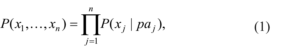
A graph (or a network) is a mathematical structure used to represent the relations among a set of elements. Formally, a graph $G = (V, E)$ consists of a set $V$ of nodes (or vertices) and a set $E$ of edges (or links), which encode the connections between pairs of nodes (Newman, 2018). Each node $v \in V$ is associated with one random variable $X_{i}$ . The edges in a graph can be directed or undirected, and weighted or unweighted, depending on the relationship represented. Graphical models have been used to encode different kinds of relationships, for example, patterns of friendship among individuals, data connections in the Internet, or predatory interactions among species (Newman, 2018). In these examples, the edges in the graph represent observed relationships (friendship, connectivity and predation). However, graphical models have also been used to represent relationships that are not directly observed, but are estimated from data.

Researchers in the social and behavioral sciences have long used causal graphical models to represent systems of causal relationships (e.g. Bollen, 1989; Morgan and Winship, 2015). In particular, a large body of empirical work in these fields uses structural equation models (SEM), which are comprised of a causal graph $G$ over a set of variables $X$ , and a joint distribution $p$ over $X$ (Glymour et al., 2019). The graph $G$ is typically a directed acyclic graph (DAG) that encodes the investigators’ understanding of the causal relation among the variables of interest. A DAG can support a causal interpretation, in the sense that for any directed edge $e = X_{i} \to X_{j}$ in $E$ , $X_{i}$ is a direct cause of $X_{j}$ relative to the variables in $V$ (Eberhardt, 2017). Following the standard definition of a causal effect, $X_{i} \to X_{j}$ implies that there is an intervention on $X_{i}$ that will directly change the distribution or value of $X_{j}$ (Glymour et al., 2019).

One of the main purposes of SEM is to examine whether a hypothesized model $G$ is consistent with the observed distribution $p$ . Another key objective is to use $p$ to estimate the magnitude of the hypothesized relationships among the variables in $G$ (e.g. Bollen, 1989). It is worth noting, then, that all applications of SEM assume that $G$ is known. In many cases, however, the underlying data-generating processes is not well understood, or prior knowledge is not detailed enough to specify the structure of the DAG (Scutari and Denis, 2014).

The under-specified nature of prior knowledge becomes more apparent when we transition from monocausal to multi-causal (or system-level) explanations, as the space of possible DAGs scales exponentially with the number of nodes (Peters et al., 2017). For example, while one can construct 25 different DAGs with 3 variables, with 10 variables one can construct 4175098976430598143 different DAGs (Peters et al., 2017). The size of the search space makes it impossible to rely exclusively on prior knowledge (as well as single experiments) to construct system-level graphs (Eberhardt et al., 2012).

In sum, when considering a large number of variables, relying exclusively on expert knowledge or experimental evidence will likely be insufficient for constructing a causal graph. In this case, the structure of the graph cannot be longer assumed, and must become the object of investigation. Causal discovery or structure learning is the problem of estimating the parameters describing a graphical causal structure from observational data (Glymour et al., 2019). The basic strategy behind these methods is to identify the causal structures that are consistent with the statistical associations observed in the data.

Inferring causal relationships from observed associations is a difficult task for several reasons, notably the large search space and the potential violations of the algorithms’ assumptions (e.g. the absence of hidden confounders, cycles or selection bias in the data). Despite these complications, causal search algorithms can provide useful information regarding the underlying causal structure (see, e.g. Aliferis et al., 2010; Shen et al., 2020; Spirtes et al., 2000). Below, I briefly review the goals and assumptions of common causal discovery algorithms (for more in-depth treatments, see Glymour et al., 2019; Peters et al., 2017; Spirtes et al., 2000).

Basic principles of structure learning algorithms

Structure learning algorithms rely on certain assumptions that connect causal relations to probability distributions. The first assumption is the Causal Markov Condition (CMC), which states that, in the absence of hidden confounders, all variables are independent of their non-effects conditional on their direct causes (Spirtes et al., 2000). This is a fundamental component in our understanding of causality and a common assumption in empirical research—reflected, for example, in the common injunction against conditioning on a mediator when one is interested in estimating a total effect (Glymour, 2006). Intuitively, the CMC states that the proximal processes influencing a variable $X$ “screen off” distal processes that influence $X$ via those proximal mechanisms (Glymour et al., 2019).

The CMC ensures that every distribution produced by a causal graph has the independence relations implied by the graph. However, in order to infer causal relations from observed associations we also need to assume that the statistical independencies in the data only contain the independencies implied by the graph (the so-called faithfulness assumption). By assuming that the observed distribution $p$ is Markovian and faithful to the underlying DAG, we obtain a one-to-one correspondence between the conditional independencies implied by the graph and the independencies observed in the data.

Based on these assumptions, the graph structure can be recovered from the joint distribution, that is, there is structure identifiability (Peters et al., 2017). It is worth noting, however, that the conditional independence relations implied by the data can be consistent with multiple DAGs. A set of graphs implying the same conditional independencies are called Markov equivalent, and are represented by a completed partially directed acyclic graph (CPDAG; Spirtes et al., 2000).

Researchers have proposed several algorithms that can be used to (partially) identify the underlying causal structure using observational data. In general, causal search algorithms can be divided into two groups, constraint-based and score-based (Scutari and Denis, 2014). Constraint-based algorithms use conditional independence tests to assess the presence of individual edges. Score-based algorithms, on the other hand, try to maximize a fit score assigned to the entire graph.

For example, the fast greedy equivalent search (FGES) algorithm—which I implement in the empirical application– has two stages. In the first phase, it adds edges until it maximizes a goodness-of-fit statistic (e.g. BIC). In the second phase, it removes edges until the score is no longer improved (Chickering, 2002). Compared to constraint-based methods, FGES is more computationally efficient, and score-based methods often perform better than constraint-based methods (e.g. Nandy et al., 2018; Shen et al., 2020). These are the main reasons why I implement FGES in the empirical section.⁵

Describing a network’s structure

Structure learning methods provide a principled way of constructing a causal graph when the data-generating process is not well understood or when prior knowledge is not detailed enough. Once the causal structure has been estimated, researchers have been typically interested in predicting how intervening on some variable $X$ affects an outcome $y$ . Causal graphs are mainly used in this context to assess the identifiability of such causal effects (Morgan and Winship, 2015; Pearl, 2009). In this section, I show how an estimated causal graph⁶ can be used to shed light into structural questions related to structural proximity, cohesion and importance.

Measuring structural proximity

Graphical models allow us to decompose the joint distribution of the data in terms of smaller distributions involving a subset of variables. In particular, the Causal Markov Condition (CMC) implies that, given a causally sufficient set of variables $V = {X_{1}, \dots, X_{n}}$ and a DAG $G$ representing the causal structure of $V$ , then the joint probability distribution can be factored as follows:

P (x_{1}, \dots, x_{n}) = \prod_{j = 1}^{n} P (x_{j} | p a_{j}),

(1)

where $p a_{j}$ represents the “parents” or “direct causes” of $x_{j}$ in $G$ . Equation (1) is consistent with the intuition that direct causes “screen off” more distal causes (i.e. if we know the direct causes of $x_{j}$ , then any other cause will not give us any additional information regarding $x_{j}$ ; Pearl, 2009).

A graph that satisfies the CMC provides immediate information about structural proximity. In particular, from a causal perspective the adjacent nodes can be interpreted as the direct causes or “proximal mechanisms” of a target variable among the set of variables considered. Identifying proximal mechanisms has long been a key objective in the social and behavioral sciences, as they help investigate and explain the phenomena under investigation, guide effective interventions, and obtain stable and accurate predictions of the target variable (Quintana, 2020).

Measuring structural cohesion

A multicausal framework starts with the premise that causal factors typically do not operate in isolation. Following this approach, a more realistic conceptualization of causal mechanisms is as “mechanistic property clusters” (MPC), defined as a set of factors that typically “hang together” because of underlying causal processes (Kendler et al., 2011).

The concept of MPC has gained some momentum in psychology, as researchers have argued that most psychological constructs do not refer to well-defined natural classes or “essences,” but rather to multi-factorial and fuzzy sets of mutually reinforcing factors (Borsboom et al., 2019; Fried, 2017). Yet, as Kendler et al. (2011) explain, the fact that causal mechanisms are fuzzy and multi-factorial does not mean that they are intrinsically unstable. On the contrary, clusters of mutually reinforcing factors might be more stable than single factors, as other factors can counterweigh the effect of localized changes.

Given that network analysis examines the properties that arise from the connections among different elements in a system, it has been considered an adequate tool for understanding how the causal interactions of micro-level components give rise to meso-level properties such as MPC’s (e.g. Borsboom et al., 2019; Schmittmann et al., 2013). A concept that can be particularly helpful in investigating the organization of a network at a mesoscopic level (i.e. at an intermediate level between the network as a whole and the individual nodes) is the idea of structural cohesion. Specifically, if we assume that nodes within MPCs are more likely to be connected than nodes belonging to different MPCs, then one can use methods for measuring cohesion such as community detection algorithms for identifying potential MPCs.

The general objective of community detection algorithms is to find groups or clusters of nodes that are densely connected internally and sparsely connected externally (Newman, 2018). Several algorithms have been developed, without clear consensus on which algorithms should be preferred under different scenarios. Furthermore, these algorithms are typically not applied to causal graphs. Thus, in the empirical section I implement some of the highest-performing algorithms, according to different comparative studies. In Section 1 of the Supplemental Appendix, I review the main ideas behind the algorithms that I implement: the Louvain, Infomap, and Walktrap algorithms.

Measuring structural importance

As explained above, researchers have defined the importance of a cause in terms of the extent to which the cause affects the outcome through multiple pathways (often referred to as a “fundamental cause”). The idea is that if a cause intervenes in many causal pathways, then it will more likely be a necessary and/or sufficient cause. According to this perspective, in order to assess the causal importance of a variable we need to understand the role it plays in the system. More specifically, we need to assess the extent to which the variable participates in many causal pathways.

In network analysis, centrality measures are used for quantifying the importance of a node. Some of the most common centrality measures are degree, closeness and betweenness (see equations 2A, 3A and 4A in the Supplemental Appendix). In essence, degree centrality measures the number of edges directly connected to a node; closeness centrality measures the average distance of a node to all other nodes; and betweenness centrality measures the extent to which a node lies on the shortest path between other pairs of nodes.

It is worth noting that none of these three centrality indices can be considered a measure of fundamental causality. To begin with, the theory of fundamental causality is typically applied to particular causes and effects (e.g. socioeconomic status and health disparities), that have well-identified intervening mechanisms (e.g. Phelan et al., 2010). In the present application, the centrality measures are used as an exploratory tool to shed light into the importance of variables within a complex system.

Despite these differences, the three centrality measures have theoretical similarities with the concept of fundamental causality. A cause can be considered “fundamental” if it affects a particular outcome through multiple mechanisms (Lutfey and Freese, 2005). This implies that the cause (1) must have several immediate effects, and (2) these effects must be connected in a proximal or distal way with a particular outcome. Degree centrality evaluates the first condition: for example, if a variable has a degree of one (i.e. it is only causally related to another variable), then it is unlikely that it is a fundamental cause. Closeness and betweenness centrality evaluate both conditions: a node with high closeness implies that it is proximally related to many variables, whereas a node with high betweenness implies that it is involved (e.g. as a mediator) in many causal pathways.

Centrality measures make implicit assumptions about the flow of the process represented in the network (Borgatti, 2005). In particular, closeness and betweenness centrality are based on the concept of shortest path, which does not have a clear theoretical correspondence in causal systems. In fact, the concepts of “flow” and “distance” are themselves problematic in the context of causal processes—strictly speaking, there is nothing that “flows” in a causal process.

Given that the assumptions underlying common centrality measures are difficult to defend (or even interpret) when applied to causal graphs, researchers have suggested that we should “leave the idea of centrality indices behind completely” (Bringmann et al., 2019, p.899). As the authors note, trying to find the most central variable is contrary to the core principle of the network approach, namely the idea that a causal system can only be understood from a structural or system-level perspective, and that interventions might be better directed at clusters rather than single factors.

The present study is sympathetic with leaving the idea of centrality behind, as well as the wish of finding the most important variable (or variables) in the system. This approach not only relies on very strong and potentially implausible assumptions, but it can also lead to misconceptions regarding the complex processes underlying social and behavioral systems (for another critical assessment of centrality measures in psychology see Neal and Neal (2021)).

Yet I also recognize the possibility that some factors—or, more likely, clusters of factors—are more central than others. As noted above, researchers have long recognized that some causes have an overriding and wide-ranging effect, which persists even after major transformations in other parts of the system. A clear example of this type of cause is socioeconomic status (SES), which is linked to persistent disparities in multiple domains—for example, the behaviors affected by low SES have been referred to as “the behavioral constellation of deprivation” (Pepper and Nettle, 2017).

Centrality measures provide a way of assessing the importance of nodes based on their structural characteristics. For illustration purposes, I will apply the three centrality measures to the estimated causal skeleton (i.e. an undirected graph), as well as to a directed DAG. However, it is worth stressing that this application relies on strong assumptions related to the direction of the edges, the absence of confounders and the absence of cycles (which generates undefined distances). Thus, inferences regarding structural importance will be less stable than inferences regarding proximity and cohesion, and should be interpreted with caution.

Based on the directed graph, I will compute the degree, the closeness and the betweenness centrality. The degree refers to the number of edges from a particular node. The reason to focus on the out-degree is that we want to identify important causes (rather than, e.g. multi-determined effects). The same rationale applies to closeness and betweenness. In this case, the shortest paths will only include edges that point in the direction of the arrowheads. Thus, in the directed graph closeness measures the degree to which a variable is a proximal cause of other variables, and betweenness the extent to which a variable stands as a mediator in multiple paths.

Data

The data comes from the Early Childhood Longitudinal Study (ECLS-K:2011) conducted by the National Center for Education Statistics (see Tourangeau et al., 2018, for more information regarding this study). The study tracks a nationally representative sample of 18,170 U.S. children who entered kindergarten in the 2010–2011 school year through fifth grade. Sampling weights are provided in the data set in order to account for differential selection at each sampling stage and to adjust for the effects of nonresponse (Tourangeau et al., 2018). In this study, the analytic sample was defined as 5792 individuals that had a valid sampling weight that maximized the number of sources included in the analysis (which involved child, parent, teacher, and school administrator data from multiple waves).

The objective of the ECLS: 2010 study was to “measure children’s experiences within multiple contexts and development in multiple domains,” and as a consequence collected data “on a wide array of topics at a broad level rather than on a select set of topics in more depth” (Tourangeau et al., 2018: 2–3). Thus, the design of the study included collection of information “from the children, their parents or guardians, their teachers, their schools, and their before- and after-school care providers” (Tourangeau et al., 2018). The wide scope and coverage of this study makes it ideal for an ecological (or structural) analysis, which intends to understand how the main causal factors in a system relate to each other.

Variable selection was guided by two general considerations. First, the variable should be considered an important factor in child’s development according to the existent research. Second, the variable is conceptually distinct from all other variables.⁷ In the empirical analysis, I included 91 variables, which can be broadly classified in the following categories: children’s demographic characteristics (5), cognitive skills (12), socioemotional behaviors (27) and habits (4); family socioeconomic status, composition and dynamics (15); instructional variables related to the curriculum, pedagogy and time spent on different activities (17); and school (10) and neighborhood (1) characteristics. Table 1 presents all the variable abbreviations along with their category, scale, measurement procedure and measurement occasion (for a more comprehensive description of most variables, for example, related to the validity and reliability of the measurement instruments used, see Tourangeau et al., 2018). The dataset included 74 continuous and 17 categorical variables (see the Supplemental Appendix for information related to the data pre-processing).

Table 1.

Description of the 91 variables included in the analysis.

Abbreviation	Construct	Type	Continuous	Measurement procedure	Measurement occasion (grade)
age	Age at assessment	Demographic	Yes	Collected from administrative data and child assessments	3rd
bmi	Body mass index	Demographic	Yes	Calculated by ECLS	3rd
disability	Disability status	Demographic	No	Collected from PI	3rd
sex	Sex	Demographic	No	Collected from school and PI	3rd
race	Race/ethnicity	Demographic	No	Collected from PI and the Field Management System	3rd
approach	Approaches to learning	Cognitive	Yes	7 items from TQ	3rd
attention	Attentional focusing	Cognitive	Yes	6 items from TQ	3rd
control	Inhibitory control and attention	Cognitive	Yes	Task composed of 20 trials	4th
grit	Perseverance over the long term	Cognitive	Yes	6 items from CQ	5th
intmath	Perceived interest/competence in mathematics	Cognitive	Yes	5 items from CQ	3rd
intread	Perceived interest/competence in reading	Cognitive	Yes	5 items from CQ	3rd
intscience	Perceived interest/competence in science	Cognitive	Yes	5 items from CQ	3rd
math	Knowledge and skills in reading in mathematics	Cognitive	Yes	Mathematics assessment	3rd
reading	Knowledge and skills in reading in reading	Cognitive	Yes	Reading assessment	3rd
science	Knowledge and skills in reading in science	Cognitive	Yes	Science assessment	3rd
workmem	Working memory	Cognitive	Yes	Task composed of 30 items	3rd
cogflex	Cognitive flexibility	Cognitive	Yes	Task composed of 40 trials	3rd
schbelong	School belonging	Socioemotional	Yes	5 items from CQ	5th
engage	Behavioral engagement	Socioemotional	Yes	5 items from CQ	4th
externalize	Externalizing problem behaviors	Socioemotional	Yes	6 items from TQ	3rd
incontrol	Inhibitory control	Socioemotional	Yes	7 items from TQ	3rd
internalize	Internalizing problem behaviors	Socioemotional	Yes	4 items from TQ	3rd
interp	Interpersonal skills	Socioemotional	Yes	5 items from TQ	3rd
intpeers	Perceived interest/competence in peer relationships	Socioemotional	Yes	6 items from CQ	3rd
lifesat	Life satisfaction	Socioemotional	Yes	6 items from CQ	3rd
lonely	Loneliness	Socioemotional	Yes	3 items from CQ	4th
peervict	Peer victimization	Socioemotional	Yes	4 items from CQ	3rd
prosocial	Prosocial behavior	Socioemotional	Yes	3 items from CQ	3rd
socanxiety	Social anxiety/Fear of negative evaluation	Socioemotional	Yes	3 items from CQ	3rd
schlike	School liking	Socioemotional	Yes	7 items from TQ	4th
sfcontl	Self-control	Socioemotional	Yes	4 items from TQ	3rd
socialpeers	Prosocial with peers	Socioemotional	Yes	5 items from TQ	3rd
socskills	Social skills with peers	Socioemotional	Yes	4 items from TQ	4th
peerspt	Peer social support	Socioemotional	Yes	6 items from CQ	4th
strucplay	Physical activity during structured play time	Socioemotional	Yes	1 item from TQ	3rd
unstplay	Physical activity during unstructured play time	Socioemotional	Yes	1 item from TQ	3rd
schstress	Worry/stress about school	Socioemotional	Yes	5 items from CQ	5th
tconflict	Conflict with teacher	Socioemotional	Yes	8 items from TQ	3rd
tclose	Closeness with teacher	Socioemotional	Yes	7 items from TQ	3rd
aggressor	Peer victimization (child as aggressor)	Socioemotional	Yes	4 items from TQ	3rd
victim	Peer victimization (child as victim)	Socioemotional	Yes	4 items from TQ	3rd
excluded	Excluded by peers	Socioemotional	No	4 items from TQ	3rd
schavoid	School avoidance	Socioemotional	No	5 items from PQ	4th
vidgame	Time spent playing videogames	Habit	Yes	1 item from PQ	3rd
tvtime	Time spent watching TV	Habit	Yes	1 item from PQ	3rd
mediause	Media usage	Habit	Yes	3 items from CQ	4th
exercise	Time spent exercising	Habit	Yes	1 item from PQ	3rd
homelit	Home literacy environment	Family	Yes	3 items from PQ	2nd
housetotal	Total number of household members	Family	Yes	Collected from PI	3rd
pincome	Household income	Family	Yes	Collected from PI	3rd
parented	Parent education level	Family	Yes	Collected from PI	3rd
noneng	Primary language in the child’s home	Family	No	Collected from PI	2nd
numbooks	Number of books the child has	Family	Yes	1 item from PQ	3rd
pstrain	Parental strain	Family	Yes	4 questions from PI	1st
pcomm	Parent-child communication	Family	Yes	6 questions from PI	3rd
pdepress	Parental depression	Family	Yes	12 questions from PI	3rd
pexpect	Parental academic expectations of the child	Family	Yes	1 question from PI	3rd
pwarm	Parental warmth	Family	Yes	4 questions from PI	3rd
foodsecty	Household’s food security status	Family	No	10 questions from PI	3rd
spank	Frequency in which the parent spanked the child	Family	No	1 item from PQ	Kindergarten
pdivorce	Parental divorce or separation	Family	No	1 item from PQ	3rd
monitoring	Parental monitoring	Family	Yes	3 items from CQ	5th
famstruc	Types of parents in the household	Family	No	Collected from PI	3rd
flldirections	Teacher’s attention to the child’s direction-following ability	Instruction	No	1 item from TQ	3rd
timeart	Time spent in art, music and physical education	Instruction	Yes	6 items from TQ	2nd
timemath	Time spent in mathematics	Instruction	Yes	1 item from TQ	2nd
timeread	Time spent in reading and language arts	Instruction	Yes	1 item from TQ	2nd
timescisoc	Time spent in science and social studies	Instruction	Yes	2 items from TQ	2nd
freetime	Time for unstructured activities (playing and lunch)	Instruction	Yes	2 items from TQ	3rd
hmwkread	Time dedicated to homework	Instruction	Yes	2 items from TQ	3rd
indepwork	Time spent on individual work	Instruction	Yes	4 items from TQ	2nd
tchcenter	Time spent on teacher-centered instruction	Instruction	Yes	1 item from TQ	2nd
schrecess	Time dedicated to recess	Instruction	Yes	2 items from TQ	3rd
stdtests	Use of state or local standardized tests	Instruction	Yes	1 item from TQ	2nd
skilsmath	Coverage of mathematics skills	Instruction	Yes	32 items from TQ	2nd
skilsread	Coverage of reading skills	Instruction	Yes	33 items from TQ	2nd
whlclass	Whole-class activities	Instruction	Yes	1 item from TQ	Kindergarten
chcenter	Child-centered activities	Instruction	Yes	1 item from TQ	Kindergarten
quizzes	Use of classroom tests or quizzes	Instruction	Yes	1 item from TQ	2nd
tchobs	Focus on students’ mastery of objectives or standards	Instruction	No	1 item from TQ	2nd
edstand	Evaluation based on standards	Instruction	No	1 item from TQ	3rd
blwmath	Students below grade level in mathematics	School	Yes	1 item from TQ	3rd
blwread	Students below grade level in reading	School	Yes	1 item from TQ	3rd
schsafety	School safety	School	Yes	6 items from SAQ	3rd
schnbhd	School neighborhood safety	School	Yes	6 items from SAQ	3rd
nonwhite	Percent of non-white students in the school	School	No	Collected from SAQ	3rd
frmeal	Percent of students in the school approved for free or reduced-price meals	School	No	Collected from SAQ	3rd
schtype	School type	School	No	Collected from SAQ	3rd
location	School locality	School	No	Provided by ECLS	3rd
distpov	School district poverty	School	Yes	Collected from SAQ	3rd
nbhdsafe	House neighborhood safety	Neighborhood	Yes	3 items from PQ	Kindergarten

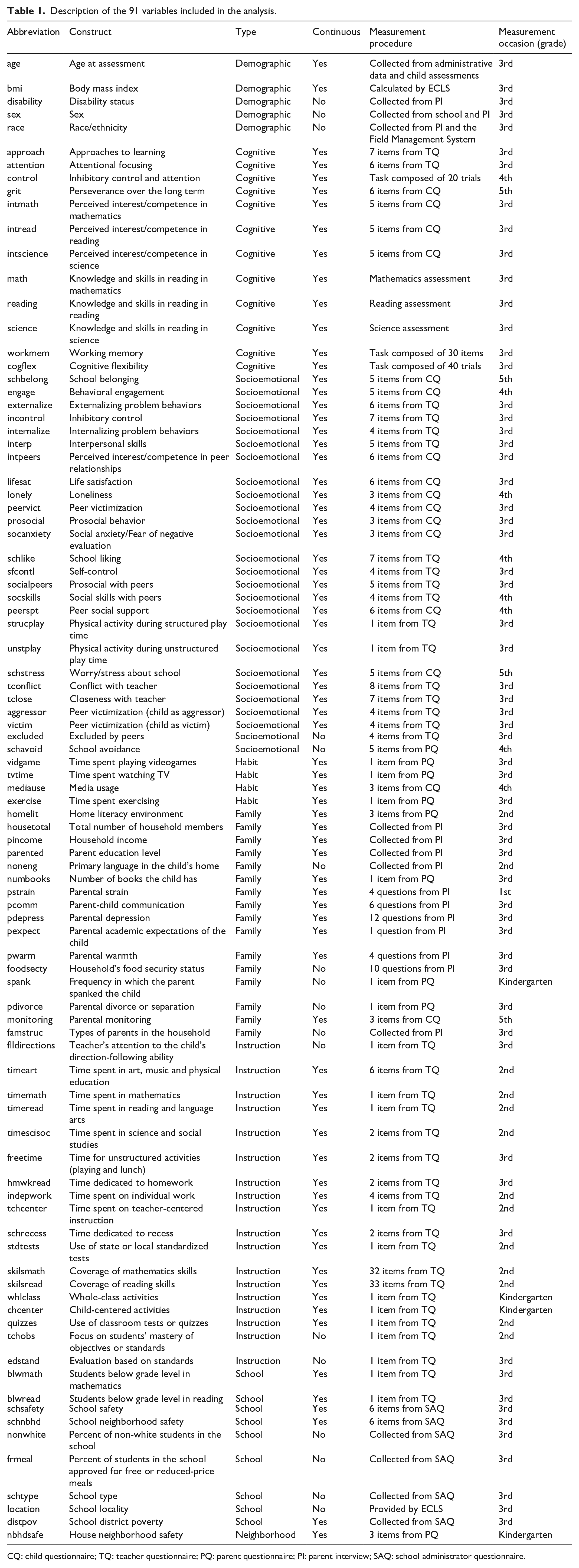
CQ: child questionnaire; TQ: teacher questionnaire; PQ: parent questionnaire; PI: parent interview; SAQ: school administrator questionnaire.

Empirical analysis

The empirical analysis was divided in two main phases. In the first phase, I estimated the causal structure of the 91 variables considered using the FGES algorithm implemented in Tetrad 6.6.0 (Spirtes et al., 2000). As explained above, the purpose of structure learning algorithms is to learn as much as possible about the causal relationships underlying a particular set of variables.

The correspondence between the conditional independencies encoded in causal structures and the probabilistic independencies found in the dataset is possible only if one makes certain assumptions, in particular the causal Markov and causal faithfulness assumptions. In addition, FGES makes the important assumption that there are no unobserved confounders in the dataset (this assumption is in fact a corollary of the other two assumptions; see Scutari and Denis, 2014). Violations of the non-confounding assumption may generate spurious edges, which will introduce bias in the estimated causal structure. As with most observational studies, assuming the non-confounding assumption is unrealistic in the present scenario. Thus, rather than interpreting the edges involving a node $X$ in causal terms as the direct causes or effects of $X$ , one can interpret the edges in purely probabilistic terms as the set of variables carrying all information in the dataset about $X$ and being directly related to $X$ .

In order to estimate network structures, researchers often use methods such as regularization to increase the sparsity of the model (Epskamp et al., 2018). A sparser model is more conservative, in the sense that it uses a smaller number of edges to explain the dependencies in the data (thus increasing the interpretability of the model). In order to increase the sparsity of the estimated network, I imposed a maximum degree of four edges.⁸

In order to indicate the lack of confidence in the presence and direction of individual edges, for most purposes I used the causal skeleton, that is, the undirected graph. In this context, the presence of an edge indicates either a hypothesized direct connection between two nodes, or a probabilistic dependence due to an unobserved confounder. I used the undirected graph in every analysis, except in the calculation of the centrality measures, where I also used a directed graph.

In the second phase, I used the graph estimated in the first stage to examine the three structural queries described above. The tools that I used to investigate these issues are related to the notions of graph distance, community detection and node centrality, respectively. All of the analyses were conducted using the igraph R package (Kolaczyk and Csárdi, 2014), and for network visualization I used Cytoscape 3.8.0 (Shannon et al., 2003).

Results

Skeleton identification

The causal skeleton (i.e. the undirected graph) underlying the 91 variables considered was estimated using the FGES algorithm. In order to increase the robustness of the results, the FGES algorithm was bootstrapped (with replacement) 500 times. If an edge (either directed or undirected) appeared in 50% or more of the bootstrap samples, then the edge was retained.

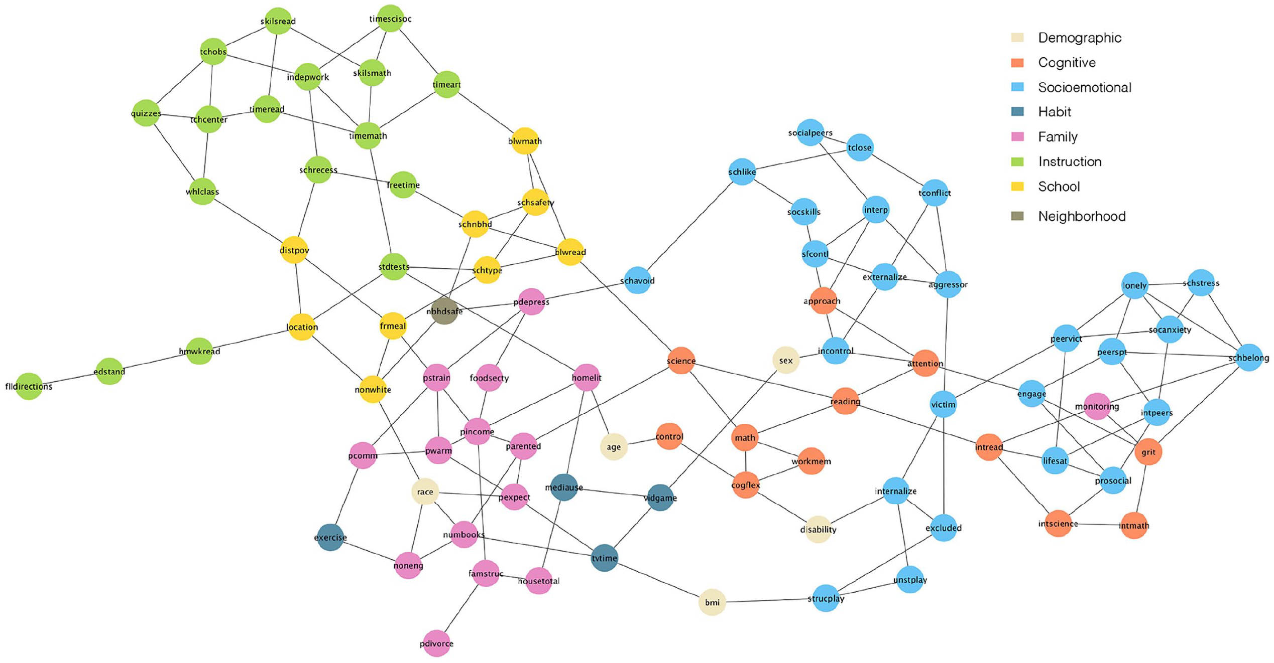
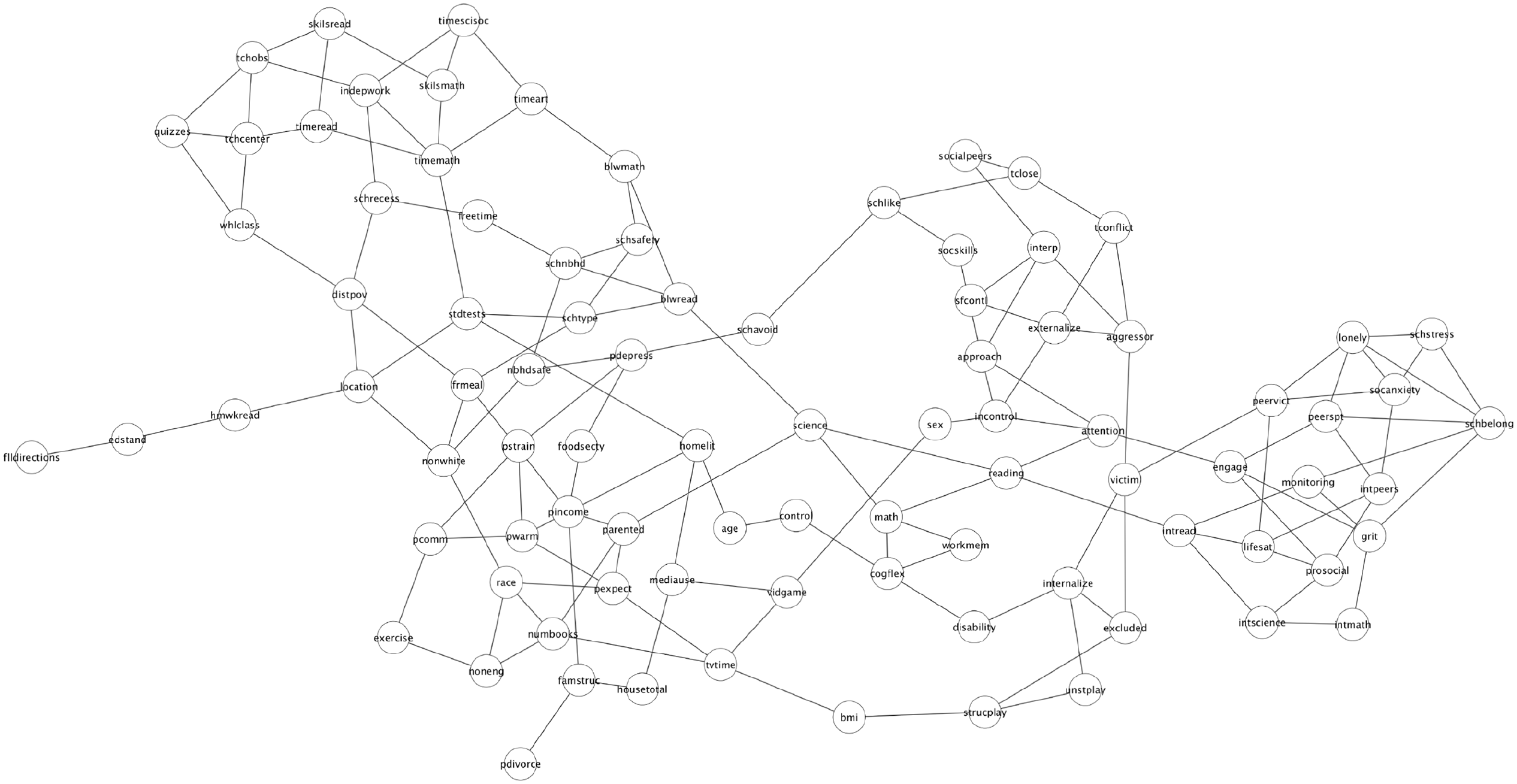
The estimated graph is depicted in Figure 1. The graph shows which variables provide information about a target variable and which variables are probabilistically irrelevant. The visualization of the graph was realized by using the prefuse force directed layout algorithm, which minimizes the crossings among edges (Heer et al., 2005). The graph has 89 nodes and 146 edges. Two nodes ( $c h c e n t e r$ and $s p a n k$ ) are missing from the graph, given that they were not connected to any other node. All subsequent analyses were performed without these two variables.

Figure 1.

Estimated causal skeleton.

In order to create a directed graph, I used the direction of the edges established by FGES. Two edges were not oriented by the algorithm: $a p p r o a c h - i n c o n t$ and $f l l d i r e c t i o n s - e d s t a n d$ . Based on background knowledge, I oriented these edges as $i n c o n t \to a p p r o a c h$ and $e d s t a n d \to f l l d i r e c t i o n s$ .

Proximal and distal relationships

One can investigate causal proximity by identifying the nodes that are directly connected to other nodes. Given that the graph depicted in Figure 1 is undirected, one cannot distinguish between the estimated direct causes or the estimated direct effects of a particular variable. If the main purpose of the analysis is to identify the direct causes (or effects) of a target variable, then it would be recommended to organize the study design for that purpose, for example by taking temporal precedence into account (e.g. Quintana, 2020).

Given that the present study is not exclusively designed for this purpose, making strong claims about proximal mechanisms of a particular variable might be unwarranted. Yet Figure 1 is consistent with prior results, according to which academic competencies (reading, math and science) are interrelated, and have direct connections to so-called executive functions (attention, working memory, and cognitive flexibility), motivation, peer academic level and parent education (see Quintana, 2020).

Apart from identifying proximal processes, the estimated graph can provide information about other questions related to proximal and distal relationships. For example, the average path length in the graph (i.e. the average shortest paths between all pairs of nodes) is 5.3. This indicates that, on average, all the nodes in the graph are connected by a minimum of around five edges. Identifying the potential mediators or colliders in a graph can be important if one is interested in estimating the causal effect of some variable on another. The diameter (i.e. the longest shortest path) in the graph includes 13 nodes.

Structural cohesion

In order to investigate the mesoscopic organization of the causal structure estimated in the first stage, three community detection algorithms were implemented: Louvain, Infomap and Walktrap. The modularity score was similar across partitions: 0.675 for Louvain, 0.682 for Infomap, and 0.685 for Walktrap. The modularity score is generally used to assess the quality of community detection methods (Newman and Girvan, 2004]; see also Section 2 in the Supplemental Appendix). A modularity score close to zero is expected when the edges are randomly formed, and a modularity score greater than 0.30 has been considered an indicator of significant community structure (Clauset et al., 2004).

I compared the agreement across the algorithms as well as with the naïve classification presented in the “type” column in Table 1 (hereafter “the naïve classification”). In order to compare the consistency across partitions one can use the Adjusted Rand Index (ARI), which is a common method for cluster validation based on which pairs of observations belong to the same cluster, adjusting for chance agreement based on cluster size (e.g. Steinley et al., 2016). The ARI is bounded between −1 and 1, with values near zero indicating chance agreement between partitions.

The Louvain algorithm found seven clusters, Walktrap 10 and Infomap 12. There is a moderately-good agreement across results, as the ARI between all methods is above 0.6 (see Table 2). On the other hand, one can observe a poor consistency between the three algorithms and the naïve classification. This suggests that community detection methods can provide information about the functional organization of the system that might not be evident from background knowledge alone.

Table 2.

Agreement among the community detection algorithms and the naïve classification (adjusted Rand index).

	Louvain	Infomap	Walktrap
Infomap	0.68
Walktrap	0.70	0.86
Naïve classification	0.36	0.34	0.32

To illustrate this point, consider the partition of the graph according to the naïve classification depicted in Figure 2. One can perceive that variables belonging to the same category tend to cluster together. However, there are variables that are directly related to variables from a different category. For example, parental monitoring, which was classified as a “family characteristic”—along with related variables such as parental communication and parental warmth—, is in fact directly related to socioemotional and cognitive variables (school belonging, grit and interest in reading). More generally, one can perceive in Figure 2 a mixture of different categories in different parts of the network (e.g. between socioemotional and cognitive attributes, or between family characteristics and children’s habits). This suggests that the naïve classification might provide insufficient or misleading information regarding the functional organization of the system in general, and the identification of mechanistic property clusters in particular.

Figure 2.

Undirected graph with the naive classification.

Even if the three algorithms differed in the specific partitions generated, they consistently identified five clusters of nodes.⁹ The agreement is presented in Figure 3 (the partition generated by each algorithm is included in the Supplemental Material). Cluster one is composed of 11 instructional and pedagogical variables related to the time teachers spend on particular skills and subjects, as well as pedagogical and assessment practices (hereafter the “instruction” cluster); cluster two is composed of 10 variables, mostly related to the demographic and socioeconomic composition of schools, as well as with the school’s location and general academic level (hereafter the “school” cluster); cluster three is composed of 12 variables, mostly associated to the child’s social skills and behaviors (hereafter the “social-behaviors cluster”); cluster four is composed of 15 variables, mostly composed of emotional and motivational constructs (hereafter the “motivation cluster”); and cluster five is composed of six variables related to the child’s physical activity and social exclusion (hereafter the “social-exclusion cluster”).

Figure 3.

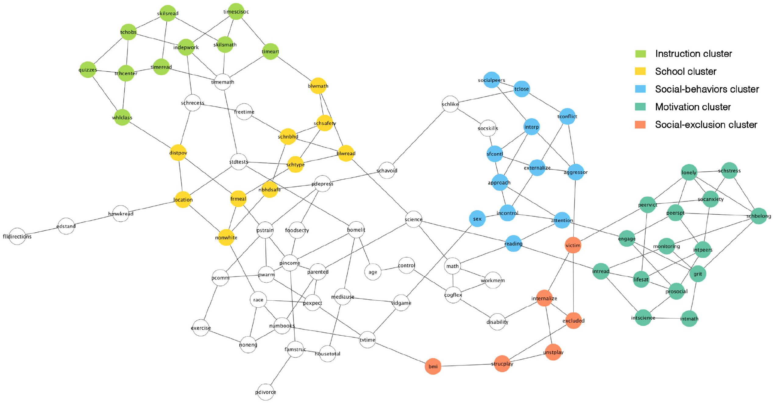
Undirected graph with the five clusters identified.

Interesting substantial conclusions can be derived from the partition depicted in Figure 3. First, the figure shows that the school cluster “shields” the instructional cluster. Probabilistically, this means that, if we are interested in predicting children’s’ developmental outcomes, then knowing the school cluster is enough, and changes in the instructional cluster do not provide any additional information.¹⁰

Second, Figure 3 can reveal relevant information regarding the causal processes associated to individual variables. For example, researchers have been interested in the construct “approaches to learning” (ATL), as it has been shown to be a very strong predictor of academic achievement (e.g. Li-Grining et al., 2010). Given that ATL assesses a range of behaviors, there is no consensus regarding the specific definition or dimensions of this construct (Buek, 2018). Based on Figure 2, one can conclude that ATL is related to other social skills and behaviors, particularly associated to self-regulation. Even if this is consistent with prior research (e.g. Li-Grining et al., 2010), researchers have also linked ATL to other skills and behavior (particularly associated to motivation and executive functions; see Buek, 2018).

More generally, the partition depicted in Figure 3 can help us identify “mechanistic property clusters,” that is, variables that typically “hang together” because of underlying causal processes (Kendler et al., 2011). In social and behavioral sciences, most variables tend to be correlated. This does not imply, however, that “everything affects everything else,” or that the correlational structure is the product of a latent common cause (e.g. van Bork et al., 2017). For example, even if academic achievement tends to be correlated with a whole range of variables—from individual-level constructs like motivation and executive functioning to school and neighborhood-level factors—, this does not imply that (1) these causal processes are structureless, or that (2) we should espouse a strong version of causal determinism, according to which the entire system is determined by one or few (latent or observed) variables. The causal structure depicted in Figure 3 suggests that, even if there are variables that tend to “hang together,” one can also differentiate among (fuzzy) clusters of variables as well as the functional organization of these clusters.

Node centrality

Inferences regarding the structural importance of specific nodes should be made with caution, due to the instability of centrality measures in the presence of missing nodes (Neal and Neal, 2021) and the sparsity constraints imposed in the search procedure. For illustrative purposes, however, the distributions of the centrality measures are presented in Figure 4. One can see that the distributions of degree and closeness approximate a bell-shape, and there is not any node that has a noticeably higher centrality. This suggests that all nodes have a similar importance in the network according to these measures. This conclusion is further supported by a low degree (0.02) and closeness (0.14) centralization (see the Supplemental Appendix for details on this metric).

Figure 4.

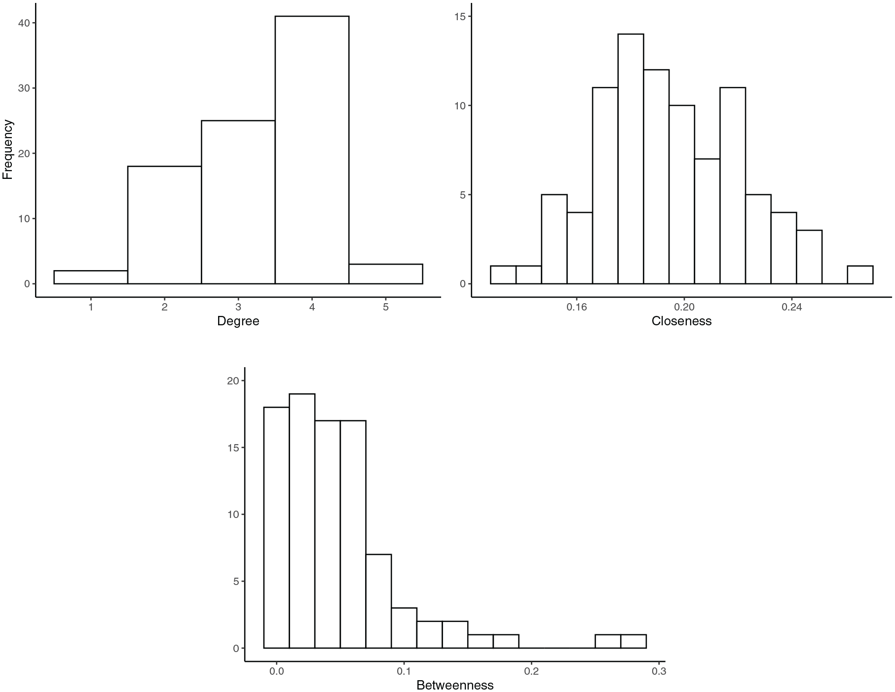
Distributions of the degree, closeness and betweenness centrality in the undirected graph.

On the other hand, the distribution of betweenness centrality has a wider range, and some nodes are more noticeably central than others. In particular, two nodes (science and reading achievement) appear to be more central according to this measure (the centrality measures by node, as well as networks sized and colored by centrality scores are presented in the Supplemental Materials). This implies that these two nodes are located at the “center” of the graph, in the sense that they lie on the path of other nodes. The more centralized structure of the network based on betweenness centrality is also reflected in a higher centralization index (0.23).

I also computed the three centrality measures using the estimated network with directed edges. As Figure 5 shows, the closeness and betweenness indices suggest that some nodes are more central than others. The former identified some cognitive skills and behaviors (reading and science achievement as well as attentional focusing) and some variables related to the child’s socioeconomic background (in particular parental income and education) as mediating several paths (e.g. based on Supplemental Table S1, both parental income and parental education are mediators in around 220 different paths). On the other hand, closeness identified several characteristics of the child’s school and socioeconomic background as being proximally related to other nodes in the network.

Figure 5.

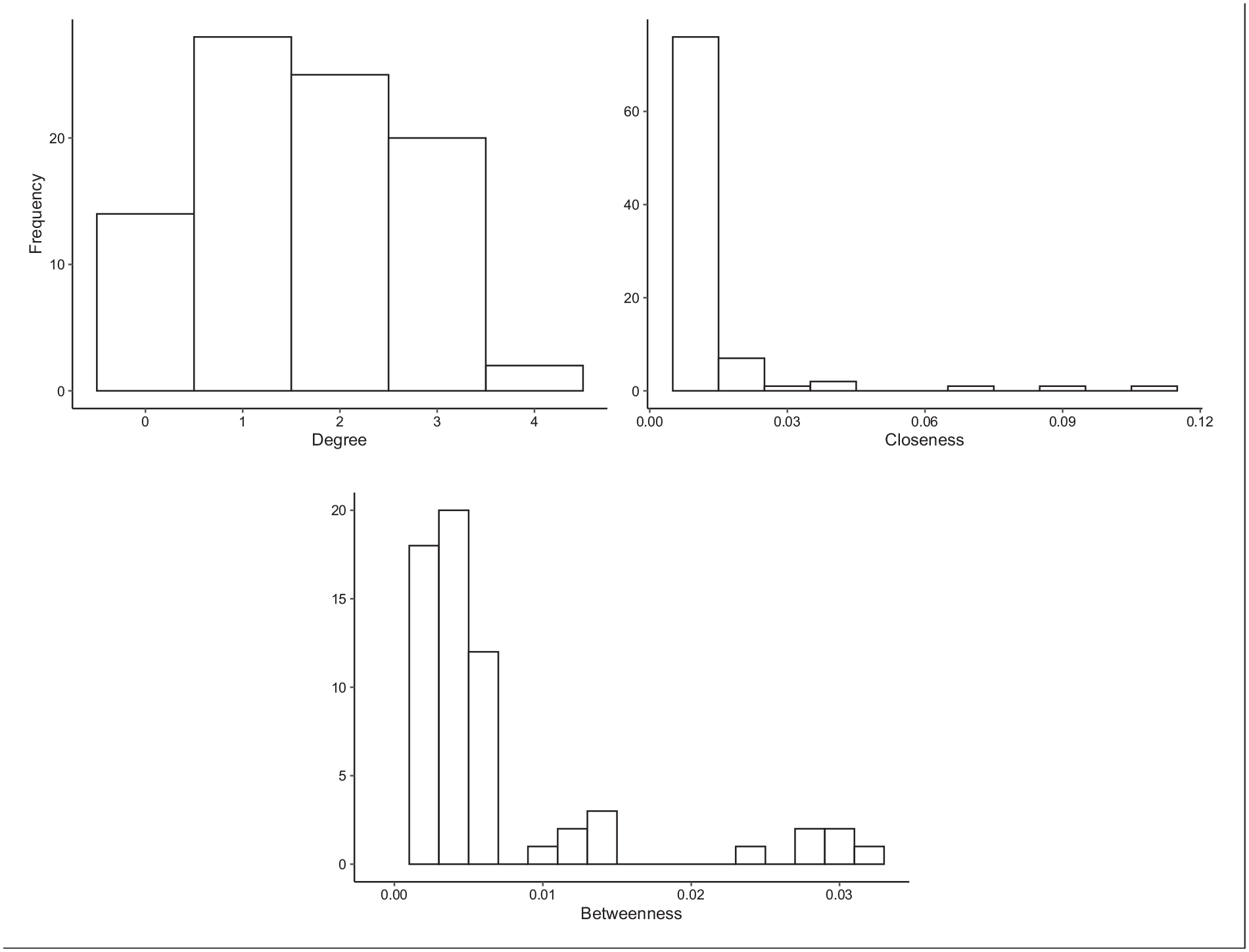
Distributions of the degree, closeness, and betweenness centrality in the directed graph.

In sum, a set of variables related to the child’s socioeconomic background and cognitive abilities (e.g. parental income and education; school district-level poverty; science and reading achievement) seem to play an important role in the network. This set of variables appears at the top in both the closeness and betweenness indices—overall, there is a strong rank correlation between these two measures, $ρ = 0.7$ . From a probabilistic perspective, this means that these nodes are more structurally informative than other nodes. From a causal perspective, this suggests that these nodes may have a relatively higher range of influence compared to more peripheral nodes.

Finally, the previous analyses also highlight the difficulty of making inferences about the importance of individual nodes using network models. Centrality indices rely on implicit and strong assumptions about the causal processes represented in the network (e.g. the absence of confounders and cycles, the direction of the edges, and the priority of shortest paths) which are impossible to validate with the existent data.

Conclusion

Even if there is a broad agreement that many problems in the social and behavioral sciences are structural in nature, there is a lack of clarity regarding what structural explanations are and how they should be formulated. In this paper, I distinguished between three types of structural inquiries related to structural proximity, structural cohesion and structural importance, and showed how descriptive analyses of causal graphs can help us investigate these issues. If researchers use these structural properties to explain a particular phenomenon then, by definition, they will be providing a structural explanation.

Adopting a structural (or ecological) approach can help us understand how different causal processes in the world relate to each other. For example, the results of the empirical application in this paper suggest that (1) executive functions, motivation, peer academic level and parent education are proximately related to academic achievement; (2) there are at least five mechanistic property clusters among the variables considered, which have different proximal or distal relationships among each other; and (3) school-level characteristics, parental socioeconomic status and academic achievement are the most central nodes in the network.

Ecological models can also dispel potential misconceptions that might arise from monocausal explanations. By explicitly portraying the interdependencies among causal mechanisms, ecological models make clear that (1) the magnitude of an effect is not the same thing as the importance of a cause; (2) an estimated average causal effect does not necessarily represent an intervention effect; and (3) in the real world, there is no such thing as a “pure” causal effect. As Bronfenbrenner (1977: 518) put it, “the principal main effects are likely to be interactions” –in the sense of multiple causes operating together. This is the reason why ecological approaches are more interested in estimating structures than causal effects.

Adopting a network perspective can also help us investigate the causal factors that researchers in the social and behavioral sciences are typically interested in, which are often vague and difficult to manipulate. Estimating the causal effect of demographic variables like race or sex, or of composite or ambiguous variables like socioeconomic status or motivation, presents insurmountable difficulties to the counterfactual framework (see, e.g. Hernán, 2016; Morgan and Winship, 2015; VanderWeele, 2016).

Furthermore, often investigations that attempt to estimate the causal effect of these variables have implicitly relied on essentialist ideas (Sen and Wasow, 2016). By attributing a causal effect to a variable (e.g. race, sex, disability status, poverty, criminal behavior, etc.), researchers might implicitly assume that these categories refer to immutable, homogenous, mutually exclusive and/or discrete natural kinds (e.g. Ahn et al., 2013; Morning, 2011). A network approach largely avoids these assumptions, as a variable is only defined relationally in terms of its position in the overall structure –but, importantly, no intrinsic or “essential” properties (e.g. a causal effect) are attributed to the variable.¹¹

In conclusion, graphical models can provide a holistic representation of the system under investigation. Contrary to other system theories, the approach presented in this paper is empirically grounded, and can generate insights and hypotheses regarding the mechanisms governing different processes in the system. A general idea of how different components of the system relate to each other can help researchers contextualize individual findings, as well as formulate more detailed questions about specific parts of the network. It is worth stressing, however, that the claim is not that ecological models are somehow superior to other explanatory approaches, but rather that they can be useful for understanding certain kinds of phenomena—that is, structural phenomena.

Supplemental Material

sj-docx-1-mio-10.1177_20597991221077911 – Supplemental material for The ecology of human behavior: A network perspective

Supplemental material, sj-docx-1-mio-10.1177_20597991221077911 for The ecology of human behavior: A network perspective by Rafael Quintana in Methodological Innovations

Supplemental Material

sj-pdf-2-mio-10.1177_20597991221077911 – Supplemental material for The ecology of human behavior: A network perspective

Supplemental material, sj-pdf-2-mio-10.1177_20597991221077911 for The ecology of human behavior: A network perspective by Rafael Quintana in Methodological Innovations

Footnotes

Declaration of conflicting interests

The author declared no potential conflicts of interest with respect to the research, authorship, and/or publication of this article.

Funding

The author received no financial support for the research, authorship, and/or publication of this article.

ORCID iD

Rafael Quintana

Supplemental material

Supplemental material for this article is available online.

Notes

Author biography

Rafael Quintana is an assistant professor in the School of Education and Human Sciences at the University of Kansas. His research interests include educational inequality, causal inference, graphical models and longitudinal analysis.

References

Ahn

Taylor

Kato

, et al. (2013) Causal essentialism in kinds. Quarterly Journal of Experimental Psychology 66(6): 1113–1130.

Aliferis

Statnikov

Tsamardinos

, et al. (2010) Local causal and Markov blanket induction for causal discovery and feature selection for classification part i: Algorithms and empirical evaluation. Journal of Machine Learning Research 11(1): 171–234.

Angrist

Pischke

J-S

(2008) Mostly Harmless Econometrics: An Empiricist’s Companion. Princeton, NJ: Princeton University Press.

Bellotti

Mora

(2016) Networks of practices in critical consumption. Journal of Consumer Culture 16(3): 718–760.

Bollen

(1989) Structural Equations With Latent Variables. New York: Wiley.

Borgatti

(2005) Centrality and network flow. Social Networks 27(1): 55–71.

Borgatti

Mehra

Brass

, et al. (2009) Network analysis in the social sciences. Science 323(5916): 892–895.

Borsboom

Cramer

AOJ

(2013) Network analysis: An integrative approach to the structure of psychopathology. Annual Review of Clinical Psychology 9: 91–121.

Borsboom

Cramer

AOJ

Kalis

(2019) Brain disorders? Not really: Why network structures block reductionism in psychopathology research. Behavioral and Brain Sciences 42: 1–63. DOI: 10.1017/s0140525x17002266

10.

Bringmann

Elmer

Epskamp

, et al. (2019) What do centrality measures measure in psychological networks? Journal of Abnormal Psychology 128(8): 892–903.

11.

Bronfenbrenner

(1977) Toward an experimental ecology of human development. American Psychologist 32(7): 513–531.

12.

Bronfenbrenner

(1979) The Ecology of Human Development. Cambridge, MA: Harvard university press.

13.

Bronfenbrenner

(1999) Environments in developmental perspective: Theoretical and operational models. In: Friedman SL and Wachs TD (eds) Measuring Environment Across the Life Span: Emerging Methods and Concepts. Washington, DC: American Psychological Association, pp.3–8.

14.

Bronfenbrenner

Morris

(2007) The bioecological model of human development. In: Lerner

(ed.) Handbook of Child Development: Vol. 1. Theoretical Models of Human Development, 6th edn. Hoboken, NJ: Wiley, pp.793–828.

15.

Buek

(2018) Approaches To Learning In The Ecls-K: Measurement And Growth From Kindergarten To Grade 2. Publicly Accessible Penn Dissertations. 2737. Available at: https://repository.upenn.edu/edissertations/2737 (accessed 15 July 2021).

16.

Chickering

(2002) Optimal structure identification with greedy search. Journal of Machine Learning Research 3: 507–554.

17.

Clauset

Newman

MEJ

Moore

(2004) Finding community structure in very large networks. Physical Review E 70(6): 066111.

18.

Cox

Mills-Koonce

Propper

, et al. (2010) Systems theory and cascades in developmental psychopathology. Development and Psychopathology 22(3): 497–506.

19.

Deaton

Cartwright

(2018) Understanding and misunderstanding randomized controlled trials. Social Science & Medicine 210: 2–21.

20.

Dunn

Schaefer-McDaniel

Ramsay

(2010) Neighborhood chaos and children’s development: Questions and contradictions. In: Evans

Wachs

(eds) Chaos and Its Influence on Children’s Development: An Ecological Perspective. Washington, DC: American Psychological Association, pp.173–189.

21.

Eberhardt

(2017) Introduction to the foundations of causal discovery. International Journal of Data Science and Analytics 3(2): 81–91.

22.

Eberhardt

Glymour

Scheines

(2012) On the number of experiments sufficient and in the worst case necessary to identify all causal relations among n variables. ArXiv Preprint ArXiv:1207.1389.

23.

Epskamp

Borsboom

Fried

(2018) Estimating psychological networks and their accuracy: A tutorial paper. Behavior Research Methods 50(1): 195–212.

24.

Freese

Kevern

(2013) Types of causes. In: Morgan

(ed) Handbook of Causal Analysis for Social Research. Dordrecht, The Netherlands: Springer, pp.27–41.

25.

Fried

(2017) What are psychological constructs? On the nature and statistical modelling of emotions, intelligence, personality traits and mental disorders. Health Psychology Review 11(2): 130–134.

26.

Fried

van Borkulo

Cramer

, et al. (2017) Mental disorders as networks of problems: A review of recent insights. Social Psychiatry and Psychiatric Epidemiology 52(1): 1–10.

27.

Frye

(1983) The Politics of Reality: Essays in Feminist Theory. Trumansburg, NY: Crossing Press.

28.

Giddens

(1986) The Constitution of Society: Outline of the Ttheory of Sstructuration, first paperback edn. Berkeley and Los Angeles: University of California Press.

29.

Glymour

Zhang

Spirtes

(2019) Review of causal discovery methods based on graphical models. Frontiers in Genetics 10: 524.

30.

Glymour

(2006) Using causal diagrams to understand common problems in social epidemiology. In: Oakes

Kaufman

(eds) Methods in Social Epidemiology. San Francisco, CA: Jossey-Bass/Wiley, pp.393–428.

31.

Gottlieb

Halpern

(2002) A relational view of causality in normal and abnormal development. Development and Psychopathology 14(3): 421–435.

32.

Hanushek

(2020) Education production functions. In: Bradley

Green

(eds) Education Economics, 2nd edn. London: Academic Press, pp.161–170.

33.

Heer

Card

Landay

(2005) Prefuse: A toolkit for interactive information visualization. Proceedings of the SIGCHI Conference on Human Factors in Computing Systems, 421–430. ACM.

34.

Hernán

(2016) Does water kill? A call for less casual causal inferences. Annals of Epidemiology 26(10): 674–680.

35.

Holt-Lunstad

(2018) Why social relationships are important for physical health: A systems approach to understanding and modifying risk and protection. Annual Review of Psychology 69: 437–458.

36.

Kendler

Zachar

Craver

(2011) What kinds of things are psychiatric disorders? Psychological Medicine 41: 1143–1150.

37.

Koedel

Mihaly

Rockoff

(2015) Value-added modeling: A review. Economics of Education Review 47: 180–195.

38.

Kolaczyk

Csárdi

(2014) Statistical Analysis of Network Data With R, vol. 65. New York: Springer.

39.

Krieger

(1994) Epidemiology and the web of causation: Has anyone seen the spider? Social Science & Medicine 39(7): 887–903.

40.

Li-Grining

Votruba-Drzal

Maldonado-Carreño

, et al. (2010) Children’s early approaches to learning and academic trajectories through fifth grade. Developmental Psychology 46(5): 1062–1077.

41.

Link

Phelan

(1995) Social conditions as fundamental causes of disease. Journal of Health and Social Behavior 35: 80–94.

42.

Lutfey

Freese

(2005) Toward some fundamentals of fundamental causality: Socioeconomic status and health in the routine clinic visit for diabetes. American Journal of Sociology 110(5): 1326–1372.

43.

Mackie

(1965) Causes and conditions. American Philosophical Quarterly 2(4): 245–264.

44.

Mahoney

(2008) Toward a unified theory of causality. Comparative Political Studies 41(4-5): 412–436.

45.

Mascolo

Fischer

(2010) The dynamic development of thinking, feeling, and acting over the life span. In: Lerner

Overton

(eds) Handbook of Lifespan Development. Hoboken, NJ: Wiley, pp.149–194.

46.

Mitchell

(2009) Complexity: A Guided Tour. Oxford: Oxford University Press.

47.

Mitchell

(2009) Unsimple Truths: Science, Complexity, and Policy. Chicago, IL: University of Chicago Press.

48.

Morgan

Winship

(2015) Counterfactuals and Causal Inference. Cambridge, MA: Cambridge University Press.

49.

Morning

(2011) The Nature of Race: How Scientists Think and Teach About Human Difference. Berkeley, CA: University of California Press.

50.

Nandy

Hauser

Maathuis

(2018) High-dimensional consistency in score-based and hybrid structure learning. The Annals of Statistics 46(6A): 3151–3183.

51.

Neal

(2013) Nested or networked? Future directions for ecological systems theory. Social Development 22(4): 722–737.

52.

Neal

(2021) Out of bounds? The boundary specification problem for centrality in psychological networks. Psychological Methods. Available at: https://psyarxiv.com/nz6k3 (accessed 10 September 2021).

53.

Newman

(2018) Networks. Oxford: Oxford university press.

54.

Newman

MEJ

Girvan

(2004) Finding and evaluating community structure in networks. Physical Review E 69(2): 026113.

55.

Pearl

(2009) Causality: Models, Reasoning, and Inference, 2nd edn. New York: Cambridge University Press.

56.

Pepper

Nettle

(2017) The behavioural constellation of deprivation: Causes and consequences. Behavioral and Brain Sciences 40: 1–72.

57.

Peters

Janzing

Schölkopf

(2017) Elements of Causal Inference. Cambridge, MA: The MIT Press.

58.

Phelan

Link

Tehranifar

(2010) Social conditions as fundamental causes of health inequalities: Theory, evidence, and policy implications. Journal of Health and Social Behavior 51 (1_suppl): S28–S40.

59.

Quintana

(2020) The structure of academic achievement: Searching for proximal mechanisms using causal discovery algorithms. Sociological Methods & Research. Epub ahead of print 10 August 2021. DOI: 10.1177/0049124120926208

60.

Reskin

(2012) The race discrimination system. Annual Review of Sociology 38: 17–35.

61.

Rothman

Greenland

(2005) Causation and causal inference in epidemiology. American Journal of Public Health 95 Suppl 1(S1): S144–S150.

62.

Rubin

(1974) Estimating causal effects of treatments in randomized and nonrandomized studies. Journal of Education & Psychology 66(5): 688–701.

63.

Sameroff

(2009) The Transactional Model. Washington, DC: American Psychological Association.

64.

Schmittmann

Cramer

AOJ

Waldorp

, et al. (2013) Deconstructing the construct: A network perspective on psychological phenomena. New Ideas in Psychology 31(1): 43–53.

65.

Scutari

Denis

J-B

(2014) Bayesian Networks: With Examples in R. Boca Raton, FL: CRC press.

66.

Sen

Wasow

(2016) Race as a bundle of sticks: Designs that estimate effects of seemingly immutable characteristics. Annual Review of Political Science 19: 499–522.

67.

Shannon

Markiel

Ozier

, et al. (2003) Cytoscape: A software environment for integrated models of biomolecular interaction networks. Genome Research 13(11): 2498–2504.

68.

Shen

Vemuri

, et al. (2020) Challenges and opportunities with causal discovery algorithms: Application to Alzheimer’s pathophysiology. Scientific Reports 10(1): 2975–3012.

69.

Skow

(2018) Causation, Explanation, and the Metaphysics of Aspect, 1st edn. Oxford: Oxford University Press.

70.

Spirtes

Glymour

Scheines

, et al. (2000) Causation, Prediction, and Search. Cambridge, MA: MIT Press.

71.

Steinley

Brusco

Hubert

(2016) The variance of the adjusted Rand index. Psychological Methods 21(2): 261–272.

72.

Thelen

Smith

(2007) Dynamic systems theories. In: Lerner

(ed) Handbook of Child Psychology. New Jersey: John Wiley & Sons, Inc, pp.258–313.

73.

Tourangeau

Nord

Lê

, et al. (2018) Early Childhood Longitudinal Study, Kindergarten Class of 2010-11 (ECLS-K: 2011): User’s Manual for the ECLS-K: 2011 Kindergarten-Fourth Grade Data File and Electronic Codebook, Public Version. Washington, DC: NCES 2018-032 National Center for Education Statistics.

74.

van Bork

Epskamp

Rhemtulla

, et al. (2017) What is the p-factor of psychopathology? Some risks of general factor modeling. Theory & Psychology 27(6): 759–773.

75.

VanderWeele

(2016) Commentary: On causes, causal inference, and potential outcomes. International Journal of Epidemiology 45(6): 1809–1816.

Supplementary Material

Please find the following supplemental material available below.

For Open Access articles published under a Creative Commons License, all supplemental material carries the same license as the article it is associated with.

For non-Open Access articles published, all supplemental material carries a non-exclusive license, and permission requests for re-use of supplemental material or any part of supplemental material shall be sent directly to the copyright owner as specified in the copyright notice associated with the article.

0.00 MB

0.03 MB

4.40 MB