
Abstract
A common research question in psychology entails examining whether significant group differences (e.g. male and female) can be found in a list of numeric variables that measure the same underlying construct (e.g. intelligence). Researchers often use a multivariate analysis of variance (MANOVA), which is based on conventional null-hypothesis significance testing (NHST). Recently, a number of quantitative researchers have suggested reporting an effect size measure (ES) in this research scenario because of the perceived shortcomings of NHST. Thus, a number of MANOVA ESs have been proposed (e.g. generalized eta squared
Effect size (ES), a quantity that directly presents or measures the strength of an effect in a study, has received increasing attention. ES is regarded as a supplement to conventional null hypothesis significance testing (NHST) because NHST focuses on making a dichotomized decision to reject or accept a research hypothesis without considering the level or magnitude of the effect observed in a study. In fact, many methodologists, professional associations, and journal editors have suggested that researchers should report ESs in addition to NHST (Murphy, 1997; Thompson, 1994; Trafimow and Marks, 2015). The American Psychological Association (APA) publication manual is more assertive on this matter, stating: “estimates of appropriate effect sizes and confidence intervals are the minimum expectations for all APA journals” (American Psychological Association, 2010: 33). The International Committee of Medical Journal Editors also states: “[a]void relying solely on statistical hypothesis testing, such as P values, which fails to convey important information about effect size.” (Mathews and Mathews, 2007, Section IV.A.6.c).
In light of the call for reporting ESs, different estimates of the true ES in the multivariate analysis of variance (MANOVA) have been developed in the literature. For example, Steyn and Ellis (2009) evaluated the accuracy of conventional MANOVA ESs (e.g. generalized eta squared
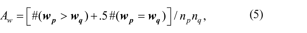
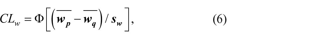
This study aims to develop a more robust ES measure (Aw) and compare it with the conventional ESs (i.e.
This paper is divided into six sections. The first section explains the importance of the two assumptions in MANOVA ESs. The second section presents the computational details of the conventional (parametric) ESs (i.e.
Two key assumptions: Multivariate normality and homogeneity of covariance matrices
In most commercial statistical packages (e.g. SPSS), four conventional NHST statistics for MANOVA are typically reported: Pillai’s Trace, Wilks’ Lambda, Hotelling-Lawley Trace, and Roy’s Greatest Root. These statistics are known to be reliable when two key assumptions are met: multivariate normality and homogeneity of covariance matrices. Multivariate normality means that a vector of weighted DV scores is independently and normally distributed for each level of the IV. Homogeneity of covariance matrices requires that the variance and covariance of the DVs are the same for each level of the IV. However, data in behavioral science often deviates from these assumptions (Keselman and Lix, 1997). Researchers in behavioral science often use single- or multi-item measures that employ Likert-scale (e.g. total score of three items each on a 5-point scale), and hence, the boundaries of the total scores are fixed (e.g. 3–15 points) producing a non-normal (i.e. platykurtic) distribution. Data observed in groups (e.g. clinical patients, gifted children) also tend to follow a heavy-tailed (i.e. skewed) distribution. Furthermore, the assumption of homogeneity of covariance matrices is rarely met in behavioral research (Tang and Algina, 1993). For example, data in a clinical group tend to have a smaller variance than in a normal group. A treatment may also be effective in systematically improving the outcome of interest among treated participants, and so they appear to be more homogenous (i.e. ceiling effect) than participants receiving no treatment.
Despite the popularity of the conventional statistics in reporting MANOVA results, previous research has found that they are not robust to violations of these important assumptions. Everitt (1979) found that these statistics tend to have an inflated Type II error (i.e. fail to reject the null hypothesis when it is false) when the degree of skewness in the DVs increases. Algina et al. (1991) found that when data are asymmetrically non-normal, the test statistics lead to inflated Type I error, especially when the covariances are heterogeneous and the sample size is unbalanced between groups. Cole et al. (1994) showed that the performance of these statistics varied. When the off-diagonal elements in the covariance matrices increase in difference across groups, the test statistics become less robust. Hopkins and Clay (1963) showed that when the covariance matrices differ between two groups, the test statistics are unlikely to be robust. Given that the conventional MANOVA ESs are based on Wilk’s Lambda, one of the conventional test statistics for MANOVA, these ESs are expected to be affected by the same assumption violations. However, no study has systematically evaluated the performance of these ES, nor has prior work proposed a non-parametric ES that does not rely on these assumptions. Here we report the first study to do both.
Conventional ESs
In two-independent samples univariate analysis of variance (ANOVA), there are two common families of ESs: the difference (d) family and correlation (r) family. For the d-family, the standardized mean difference between two groups in DV scores can be used to evaluate the strength of the effect. That is,
Generalized eta squared
In MANOVA, the generalized eta squared

where
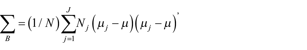
is the between-groups covariance matrix, N is the total sample size, Nj is the sample size for j = 1, 2, . . ., J groups, µj is the mean for the jth group, and µ is the grand mean. Second,
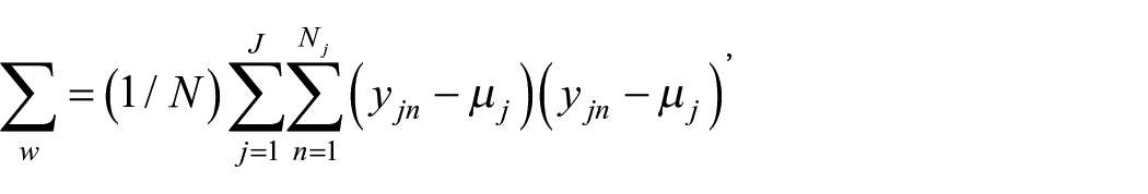
is the within-groups covariance matrix, where
Generalized omega squared
The eta squared (
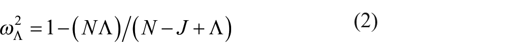
where J is the number of groups in the IV, and N and
Recently developed ESs
Parametric common language ES (CL) in ANOVA
The idea of common language ES (CL) can be found in statistical studies published almost 80 years ago when Wilcoxon (1945) proposed a rank-order comparison for scores observed between two treatments. Mann and Whitney (1947) extended Wilcoxon’s method, which calculated the rank numbers in which the scores in treatment A are larger than the scores in treatment B, by further defining the statistical properties (e.g. probability distribution) of Wilcoxon’s statistical measure, known as the U statistic. Govindarajulu (1967) was one of the early studies that formally defined the meaning of a probability estimate, P(X < Y), where X refer to continuous scores in a random sample A (e.g. treatment), and Y refer to continuous scores in a random sample B (e.g. control). This measure quantifies the probability that a score in one sample is stochastically smaller than a score in another sample. Govindarazulu focused on deriving an analytic method that constructs the confidence intervals surrounding the measure of P(X < Y). Wolfe and Hogg (1971) published a tutorial paper that encourages the use of P(X < Y) among applied statisticians and researchers.
Based on these early papers published in statistics journals, McGraw and Wong (1992) was one of the pioneer studies in psychology that proposed the use of a statistic that measures “how often a score sampled from one distribution will be greater than a score sampled from another distribution” (p. 361). They labeled this statistic a common language ES (CL) and proposed its use as a type of probability of superiority statistic for univariate ANOVA. CL estimates the parameter, P(Yp > Yq), which measures the probability that a score in group p is higher than a score in group q. For example, if a researcher is comparing the effect of an intervention group relative to a control group, the researcher can present the CL that estimates the probability (e.g. 80% chance) that the observations (e.g. self-esteem) would be better for a randomly selected member of the intervention group than for a randomly selected member of the control group. Hsu (2004) regarded this as a more intuitive way to conceptualize ES, as it is easy for researchers and practitioners to understand even without formal training in statistics. According to Ruscio (2008), when data meet the parametric assumptions (i.e. normality and homogeneity of variances), CL can be expressed as
Non-parametric A in ANOVA
Vargha and Delaney (2000) criticized McGraw and Wong’s (1992) CL on the basis that it assumes the scores follow a normal distribution. To overcome this problem they proposed a non-parametric estimator, known as the measure of stochastic superiority (i.e.

where # is the count function,
Parametric
and non-parametric Aw in MANOVA
To generalize
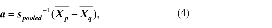
where
which expresses the probability (e.g. 90%) that the linear composite
where
This study evaluates the performance of two conventional parametric ESs—
Monte-Carlo study
Design
Seven factors that would affect the performance of
Factor 1: Standardized mean vector difference (δ; four levels)
This parameter reflects the level of standardized mean difference between the weighted DV scores in two groups, which is similar to Cohen’s standardized mean difference d in ANOVA. According to Cohen (1988), in social science research a d of 0.20, 0.50, and 0.80 reflects a small, moderate and large ES respectively. In addition, the value of 1.50 was included to examine the impact of an extremely strong δ on the observed ESs. The corresponding values for
Factor 2: Distribution (Θ; six levels)
In addition to the normal distribution (N (0, 1) with skewness (ϒ1) = 0 and kurtosis (ϒ2) = 0], five non-normal (i.e. two peaked, two skewed, and one mixed normal) distributions were generated based on Algina et al. (2005). The peaked distribution is characterized by a long (or short) tail with few (or most) scores clustered around the center of the distribution. The skewed distribution is characterized by unequal-length tails along a distribution. The mixed normal distribution appears to be a normal distribution but with longer tails on both ends, mimicking a distribution with outliers on both ends. Following Algina et al., for the peaked and skewed distributions, the normal scores were multiplied by specific g and h values so that the transformed scores followed the target non-normal distributions. Specifically, when g and h were nonzero,

where Y is the transformed score and Z is the original normal score. When g was zero,

According to Algina et al., the target peaked distributions were manipulated at (1) ϒ1 = 0 and ϒ2 = 6 (i.e. g = 0 and h = 0.142) and (2) ϒ1 = 0 and ϒ2 = 154.84 (i.e. g = 0 and h = 0.225), and the target skewed distributions were fixed at (3) ϒ1 = 2 and ϒ2 = 6 (i.e. g = 0.76 and h = −0.098; an exponential distribution) and (4) ϒ1 = 4.90 and ϒ2 = 4,673.80 (i.e. g = 0.225 and h = 0.225), which are common in social sciences research. Note that positively (or negatively) skewed distributions often have ϒ1 > 0 (or ϒ1 < 0), and shorted-tailed (or long-tailed; e.g. t distribution) distributions often have ϒ2 < 0 (or ϒ2 > 0). For the mixed normal distribution, only 90% of the observations come from the normal distribution with mean 0 and SD 1 and 10% come from the normal distribution with mean 0 and SD 10. This distribution has ϒ1 = 0 and ϒ2 = 24.95.
Factor 3: Number of DVs (ν; three levels)
Three numbers, 2, 5, and 8, were evaluated, which cover a range of values that seem to be practical in real-world research.
Factor 4: Variance ratio (π ; three levels)
Variance ratio is defined as the ratio of the variance in Group 1 to the variance in Group 2 (Ruscio and Mullen, 2012). The ratio was fixed at 1, 4, and 0.25. The value of 1 means that the variances are homogenous for the two groups, and the values of 4 and 0.25 indicate violations of the homogeneity of covariance matrices assumption, which are commonly found in social sciences research.
Factor 5: Correlations between DVs (R;
levels)
The DVs were expected to measure the same construct in MANOVA, and hence, they were manipulated to be correlated with one another in each group. Two levels of correlations, 0.50 and 0.80, were evaluated for the two groups, respectively. The value of 0.50 followed the design in Fouladi and Yockey (2002), which mimicked a moderate-to-large association between items. The value of 0.80 was included to examine the impact of extremely strong relationship. The manipulated levels in Factors 4 and 5 mimic the data conditions that meet or violate the assumption of homogeneity of covariance matrices.
Factor 6: Total sample size (N; two levels)
Two levels, 50 and 150, were simulated, thereby representing a small and moderate-large sample typically found in behavioral research.
Factor 7: Base rate (b; three levels)
In Ruscio and Mullen (2012), base rate is defined as the ratio of the sample size in Group 1 to the sample size in Group 2. Base rate was evaluated at the levels 0.25, 0.50, and 0.75. Thus, the samples sizes could be equal for the two groups, or it was three times larger in one sample than the other.
In sum, the factors were factorially combined to produce a design with
Evaluation criteria
Two evaluation criteria were used. First, for each of the 5184 simulation conditions, percentage bias (bias) was computed to evaluate the average performance of an ES relative to its true value, that is,
Results
Overall performance
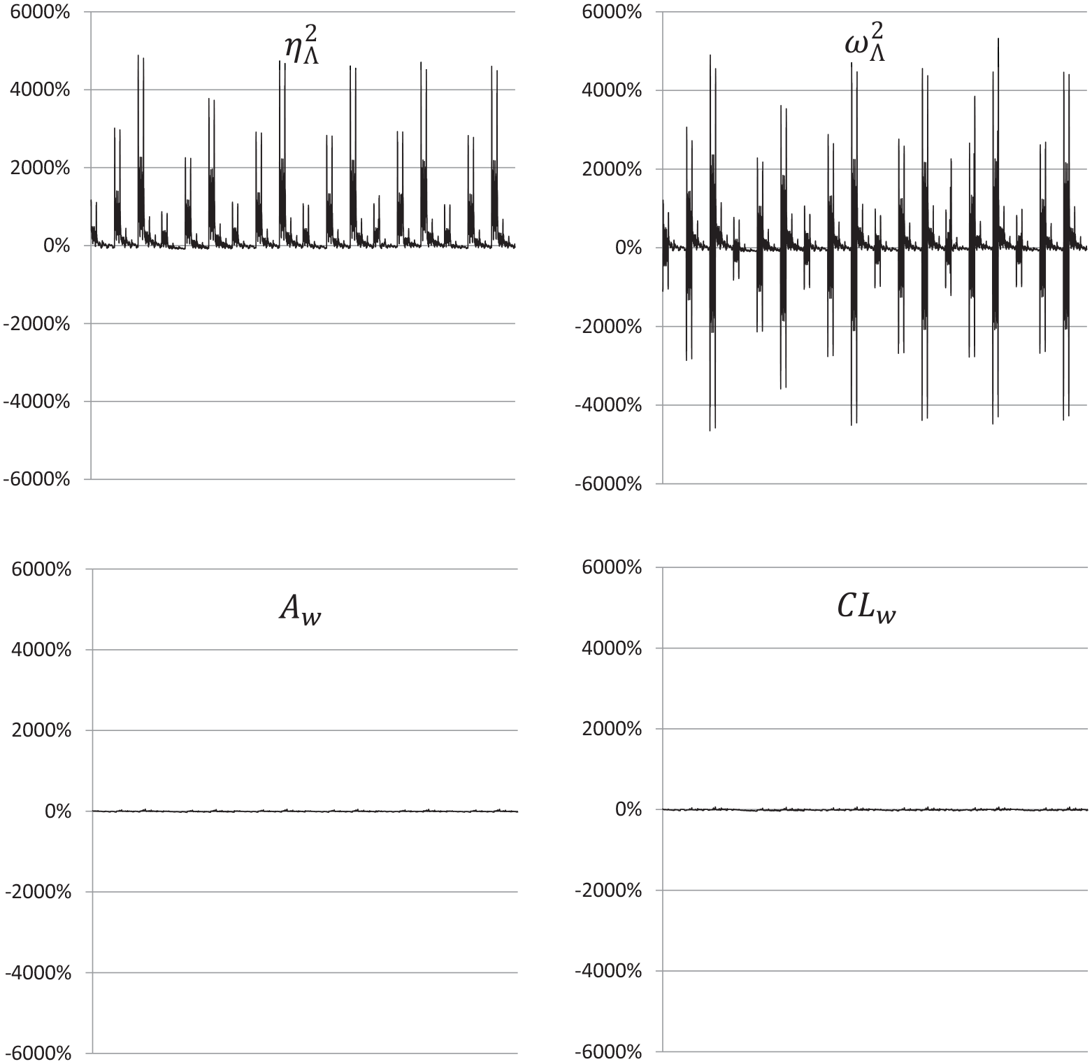
Comparing the four ESs, Aw performed the best. As shown in Figure 1, the biases ranged from −31.57% to 52.35%, with a mean of −4.16%, which is within the criterion for a good fit (
Percentage biases of the generalized eta squared (
By contrast, the conventional parametric ESs (
Note that the reason for a wide range of biases is in part due to the metrics of the true
Effects of manipulated factors
Given that the correlations between DVs (R) did not show any effects on all the ESs, their impact is not discussed in this section. As shown in Table 1, first, when the total sample size (N) increased from 50 to 150, the accuracy of
Percentage biases of
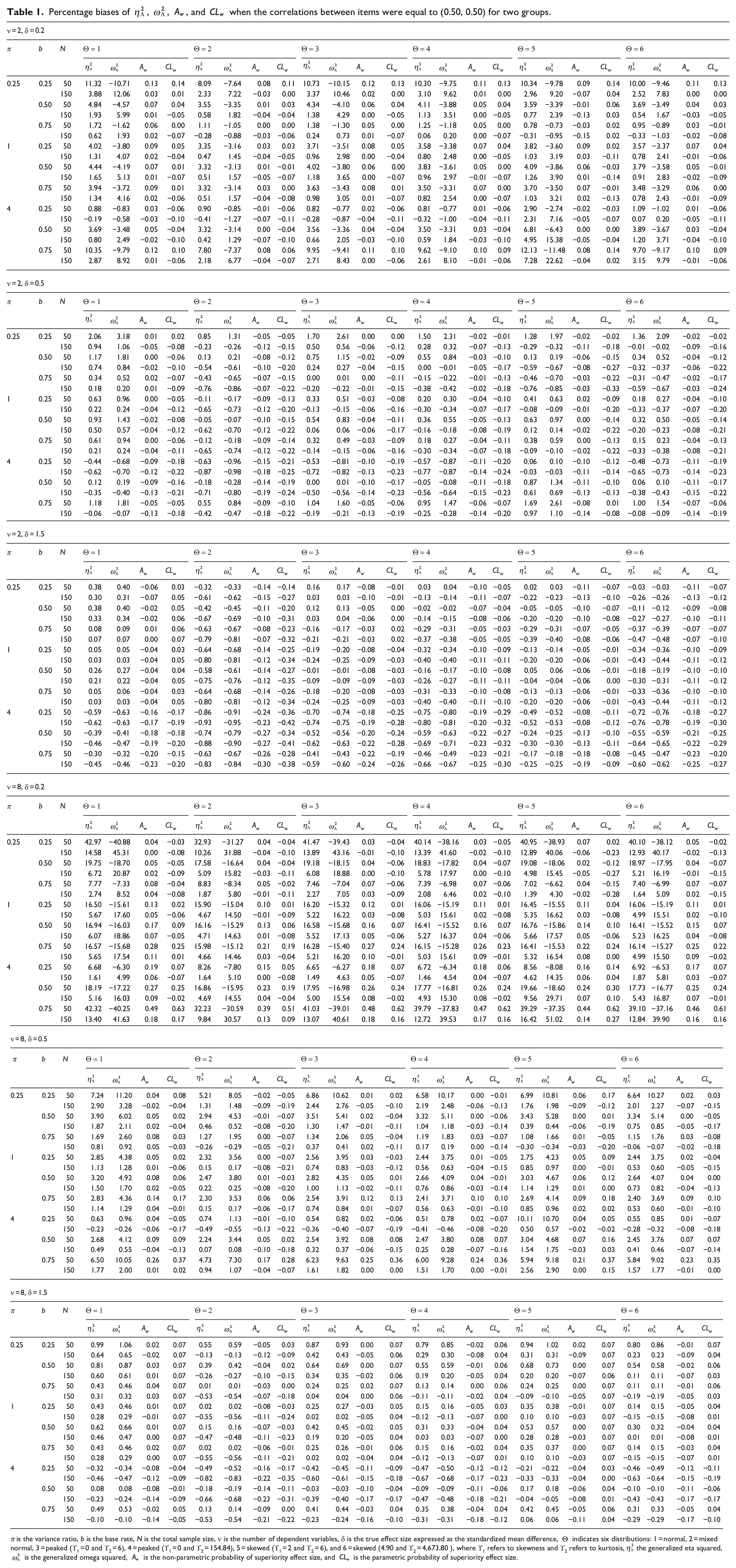
π is the variance ratio, b is the base rate, N is the total sample size, ν is the number of dependent variables, δ is the true effect size expressed as the standardized mean difference,
Second, the variance ratio (π; i.e. variance ratio of the treatment group) did not show obvious impact on Aw and CLw. For
Third, the base rate (b; i.e. proportion of the sample size of the control group) did not show a clear pattern of relationship with
Fourth, when the true ES (δ) increased, the biases of
Fifth, when the number of DVs (ν) increased, the accuracy of
Sixth, it came as a surprise that the performance of
Conclusion and discussion
This study proposes and develops a non-parametric ES (Aw) for MANOVA. The results of a Monte-Carlo simulation showed that Aw was accurate across the simulated conditions and robust to violations of the two key assumptions (multivariate normality and homogeneity of covariance matrices). It also outperformed the two conventional parametric ESs (i.e.
The proposed Aw is important for researchers in behavioral and social sciences research because evaluating the conventional ESs (
The implications of this study can be generalized to researchers and practitioners in a wide range of other disciplines, both in social and natural sciences, who often use MANOVA. For example, clinical trials researchers often examine the difference between a treatment group and a placebo group in a number of health-related criterion measures (e.g. body mass index, blood pressure). On some occasions, their data may violate the assumptions for the traditional ESs, and hence, the proposed Aw can provide a more trustworthy measure for evaluating the difference between the two groups. Biological researchers are often interested in comparing the difference between an experimental group and a control group in a lab setting (e.g. effects of room temperature and absolute zero degree on cellular motility and signaling), and they could also report Aw for this scenario.
Limitations and directions for future research
A first area of ongoing research lies in examining the effects of different distributions for the two groups of observations. In this study, the two groups of scores were assumed to follow the same (either normal or non-normal) distributions. Future research should include a simulation study to examine the effects of unbalanced distributions (e.g. normal vs skewed) on the ESs in MANOVA.
A second area of research involves generalization of the proposed Aw to the one-way MANOVA with more than two independent samples as well as to the multi-way MANOVA that involves multiple IVs (e.g. factorial and mixed designs). These more general or complicated types of MANOVA are also popular in psychology research. This study lays foundation for the non-parametric ES in a simpler MANOVA. Ruscio and Gera (2013) have recently provided the extensions of Aw to one-way ANOVA. Additional research can derive mathematical equations for one-way MANOVA based on Ruscio and Gera’s study and provide empirical evidence for this statistic based on a simulation study.
In addition to the reporting of ES, the new statistical practices suggest that researchers report the CIs surrounding a reported ES. Therefore, a third area for future research is examination of the sampling distribution or confidence intervals (CIs) surrounding the proposed Aw. Ruscio and Mullen (2012) found that the bootstrap CIs constructed for the non-parametric A in ANOVA were accurate. Further research can also examine the use of the bootstrap procedure for the CIs surrounding the proposed Aw in MANOVA.
Supplemental Material
sj-pdf-1-mio-10.1177_20597991211055949 – Supplemental material for A robust effect size measure Aw for MANOVA with non-normal and non-homogenous data
Supplemental material, sj-pdf-1-mio-10.1177_20597991211055949 for A robust effect size measure Aw for MANOVA with non-normal and non-homogenous data by Johnson Ching-Hong Li, Marcello Nesca, Rory Michael Waisman, Yongtian Cheng and Virginia Man Chung Tze in Methodological Innovations
Footnotes
Declaration of conflicting interests
The author(s) declared no potential conflicts of interest with respect to the research, authorship, and/or publication of this article.
Funding
The author(s) disclosed receipt of the following financial support for the research, authorship, and/or publication of this article: This study was funded by the University Research Grant Program (#43869) at the University of Manitoba.
Supplemental material
Supplemental material for this article is available online.
Notes
Author biographies
References
Supplementary Material
Please find the following supplemental material available below.
For Open Access articles published under a Creative Commons License, all supplemental material carries the same license as the article it is associated with.
For non-Open Access articles published, all supplemental material carries a non-exclusive license, and permission requests for re-use of supplemental material or any part of supplemental material shall be sent directly to the copyright owner as specified in the copyright notice associated with the article.