
Abstract
This article explores techniques for using supervised machine learning to study discourse quality in large datasets. We explain and illustrate the computational techniques that we have developed to facilitate a large-scale study of deliberative quality in Canada’s three northern territories: Yukon, Northwest Territories, and Nunavut. This larger study involves conducting comparative analyses of hundreds of thousands of parliamentary speech acts since the creation of Nunavut 20 years ago. Without computational techniques, we would be unable to conduct such an ambitious and comprehensive analysis of deliberative quality. The purpose of this article is to demonstrate the machine learning techniques that we have developed with the hope that they might be used and improved by other communications scholars who are interested in conducting textual analyses using large datasets. Other possible applications of these techniques might include analyses of campaign speeches, party platforms, legislation, judicial rulings, online comments, newspaper articles, and television or radio commentaries.
Introduction
This article explores techniques for using supervised machine learning to study discourse quality in large datasets. We use a modified version of the discourse quality index (DQI) (DQI 2.0) to illustrate how machine learning algorithms can be trained to accurately predict human coding behaviors, facilitating the possibility of processing huge amounts of unstructured data. We focus in particular on the text vectorization of medium-length speech acts—such as those used in legislative debates—which consist of speeches or texts typically between 300 and 10,000 characters. We differentiate this length of text from shorter ones found online, as well as longer ones in research papers or books.
Vectorization, or transforming text to data, is an important problem in the analysis of political deliberation. Speech acts can be broken up in a multitude of ways, and it is not always immediately obvious which technique to use for different use cases. In this article, we explore several techniques for vectorizing speech acts into features and training machine learning algorithms on these features. These include bag-of-words, token-embedding, ngrams, part-of-speech ngrams, vocabulary-based features, structural features, and character count. We discuss how to create and select these features to efficiently train the algorithms based on different use cases.
To illustrate these techniques, we draw on data from an ongoing study of deliberative quality in Canada’s three northern territories: Nunavut, Northwest Territories (NWT), and Yukon. These three territories make for interesting case studies because while Yukon has a party-based adversarial type legislature, Nunavut and the NWT use non-partisan legislative systems. Our study uses data from 20 years of legislative debates in the each of the three territories. To compare deliberative quality across these cases, we needed to develop a reliable measure of deliberative quality and a system for automatically coding approximately 250,000 individual speech acts. In this article, we explain the machine learning techniques that we have developed to accurately code individual speech acts on 12 independent indicators of deliberative quality.
In developing our analysis program, our objective was to rely as little as possible on rule-based indicators, allowing machine learning algorithms to combine features and weights in a much more sophisticated manner. As illustrated below, we selected an algorithm that was able to select which features would be most relevant in the thousands of features created in our five vectorization techniques. While many of the models were accurate, there were cases in which we found it useful to either revert to rules or enhance the term frequency-inverse document frequency (TF-IDF) matrix with a vocabulary of terms. The question indicator, for example, was most accurately predicted when looking only for the question mark character. The respect indicator was predicted most accurately when solely using vocabulary-based features. Others, such as narrative, obtained high levels of accuracy almost immediately, showing that there is some level of predictability in the way in which stories are inserted into parliamentary speech.
Although our focus here is on using supervised machine learning techniques to code the deliberative quality of legislative speeches, the techniques we discuss will be of interest to those who wish to analyze deliberative quality in media contexts, such as online comments, newspaper articles, and television or radio commentaries, in the analysis of political communication, such as campaign speeches, party platforms, and legislation and judicial rulings, or in other political institutions such as townhall meetings or small deliberative forums. The techniques might also be applied to other big data problems that do not have to do with deliberation but nevertheless require human-guided machine learning coding, such as the comparative analyses of legislation or journal articles.
The article proceeds as follows. In the “Measuring deliberative quality” section, we discuss different approaches to measuring deliberative quality and we outline the 12 components of the DQI 2.0. In the “Techniques for training algorithms” section, we outline various techniques for training algorithms, and we explain, in general terms, which is most appropriate for which type of classification. In the “Case studies: coding for narrative, constructive proposal, response, question, and respect” section, we discuss in detail how 4 of the 12 indicators in the DQI 2.0 were modeled using different combinations of techniques, and we briefly outline of how the remaining indicators were modeled. In each case, a different combination of techniques was necessary to achieve accurate prediction scores. The purpose of the article is to demonstrate the vectorization techniques that we have developed to measure deliberative quality in large datasets.
Measuring deliberative quality
The DQI is the most widely used system for measuring deliberative quality. In its first version (Steenbergen et al., 2003), it proposed six indicators—participation, level of justification, content of justification, respect, counterarguments, and constructive politics. Each indicator was assigned a maximum value of 1, 2, or 3 points, for a total DQI score of 14. In their demonstration of the methodology, the researchers who developed the original DQI hand-coded parliamentary speeches from the UK parliament, achieving an acceptable level of inter-coder reliability.
Since the DQI was first published, subsequent iterations of the index have sought to address some of its weaknesses, namely, subjectivity and validity. King (2009) has argued that the methodology’s reliance on human coders renders it too subjective, defeating the purpose of the system for quantifying deliberative quality. Several deliberative theorists have argued, however, that translating normative concepts, such as deliberative quality, into empirical measurements is important (Borge and Santamarina Sáez, 2016; Gold et al., 2015) chiefly because we cannot use computational analysis without quantification, and the extraction of normative insights from big datasets without the use of computers is either impossible or extremely expensive and time-consuming. Finding a way of quantifying normative constructs to allow for computation is therefore essential to further advance the social scientific study of big datasets.
As most studies of deliberative quality rely on human coding techniques, researchers are limited in the number of speech acts that might be analyzed. This is a particular problem today because over the last decade or so the number and variety of deliberative exchanges that might be analyzed, from parliamentary speeches to media debates or online comments, have increased dramatically, and this trend will only continue in the future. Several researchers have therefore begun experimenting with ways to automate discourse analysis. A notable case is Gold et al. (2015), who used proxies for four indicators of deliberative quality in an experimental setting. Similarly, Borge and Santamarina Sáez (2016) used a combination of automated and manual coding to analyze online deliberations in Spain. Another example is Fournier-Tombs and Di Marzo Serugendo’s (2020) DelibAnalysis, which used machine learning techniques to code online deliberations, particularly social media and blog posts. The researchers manually coded examples of these online posts using the original DQI and used those data to teach DelibAnalysis to accurately classify them into three categories: low, medium, or high deliberative quality.
In this article, we use a modified DQI, which we have called the DQI 2.0. As illustrated in Table 1, the index contains 12 indicators which are designed to measure both positive and negative aspects of deliberation. The interruption indicator specifies whether a speech act begins as an interruption of another. Explanation indicates whether a speaker provides a minimum level of context for the claims or opinions that are expressed. Causal reasoning indicates whether a speaker makes explicit causal connections between any observations, values, or objectives and the claims, conclusions, or recommendations that are made.
The Discourse Quality Index (DQI) 2.0.

The narrative indicator acknowledges that speakers often explain themselves, or justify their claims or values, by telling stories or personal anecdotes. The question indicator specifies whether the speaker asks others for clarifications or input. The response indicator specifies whether those who are asked questions answer them instead of speaking only about their own interests or concerns. The advocacy indicator specifies whether a speech act explicitly defends or advances the interests or claims of identifiable groups or communities. The public interest indicator, by contrast, specifies whether a speaker attempts to connect claims, policies, or recommendations to the interests of the community as a whole. Disrespect indicates speech acts which include insults, dispersions, misrepresentations, name calling, and dismissive or disrespectful statements more generally. Respect indicates statements which include explicit shows of respect, such as salutations, complements, or apologies. It is worth nothing that all of the indicators in the DQI 2.0 are independent of each other, which means that it is possible for a single speech act to be coded as containing both respectful and disrespectful statements. The counterarguments indicator specifies whether a speaker engages with critiques made by others or attempts to address or respond to counter claims, concerns, or countervailing evidence. The constructive proposal indicator is used when speakers propose solutions to shared problems, alternative options, or compromises.
Each indicator in the DQI 2.0 is binary: they are either additive, where 0 signals the absence and 1 signals the presence, or subtractive, where 0 signals the absence and –1 signals the presence. (Interruption and disrespect are the only negatively scored indicators in the DQI 2.0.) This coding scheme creates an index which runs from –2 to 10, but which may be transformed to run from 0 to 12 to facilitate interpretation.
The DQI 2.0 captures the essential features of good deliberative exchanges. On a scale of 0–12, a deliberation with an average score of 0 would consist entirely of interruptions and insults, while a deliberation with an average score of 12 would consist only of speech acts that each contains every positively scored indicator. In practice, most deliberations will have average scores somewhere between these two extremes, with better, more substantive, respectful, and constructive deliberations scoring higher than less substantive and disrespectful ones.
In this article, we build upon and refine the DelibAnalysis approach that was developed by Fournier-Tombs and Di Marzo Serugendo (2020) in two ways. First, the binary measures used in the DQI 2.0 make it possible to train the analysis program to more accurately predict the scores of human coders. This is because binary measures tend to perform better with Boolean classes: in general, the fewer the options for the classifier the more accurate it will be.
Second, we expand upon the original DelibAnalysis approach by increasing the number of possible features and creating a separate model for each indicator and each legislature. Instead of one model classifying each speech act as low, medium, or high quality, we created a program capable of generating 30 separate models—a considerable expansion in scope—using several possible feature selection techniques.
Approaching the model training indicator-by-indicator and territory-by-territory allowed for more granularity than the original DelibAnalysis would have provided. Unlike the original methodology, which was used to measure the overall quality of a social media post, the current methodology allows us to analyze different components of deliberative quality, such as whether speakers regularly ask questions of others or use narratives or stories to illustrate their claims or support their arguments. In addition, we found that parliamentary speeches lend themselves to our multi-model approach because they tend to be longer and richer than the average social media post. Thus, our approach allowed us to engage in custom feature selection and model tuning to obtain the best possible accuracy scores for each indicator from the DQI 2.0. As we will see, some models were much easier to train than others, due to the particularities of each indicator. Figure 1 outlines the eight steps that we took to train our models to accurately predict each indicator.
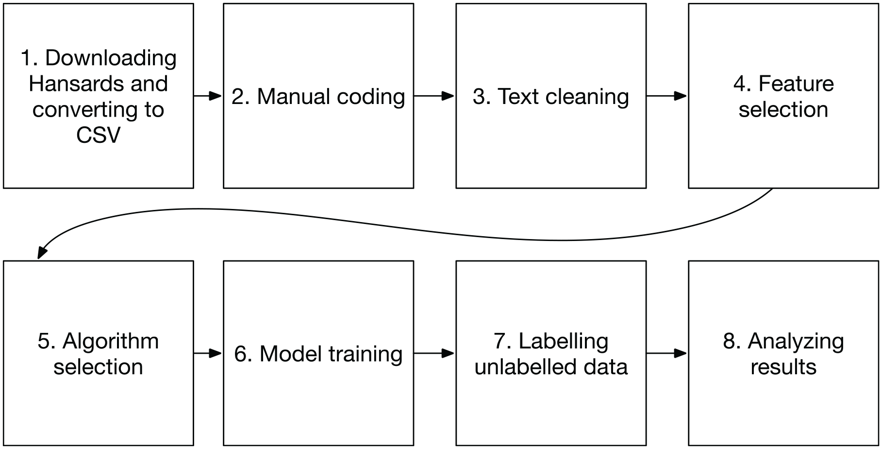
Model training and classification process.
As we illustrated above, the first step was to extract the last 5 years of Hansards from the parliamentary websites of each territory and convert them to comma-separated values (CSV) format, such that each row contains a speaker and a speech act, in sequential order for each day’s proceedings. 1 We then selected at random 200 speeches from each territory and coded them according to the DQI 2.0. We pre-processed the text as required by the model, by, for example, removing non-alphanumeric characters if necessary and converting all words to lower case. In the case of the question indicator model, we kept punctuation, notably question marks. We then chose feature selection and classification methodologies, as will be described in further detail below. We created a model and trained it using the manually coded data. We repeated the above steps and manually coded additional data until the accuracy scores for each model reached acceptable levels. (We considered 70% accuracy an acceptable threshold, 2 although several of our models achieved much higher accuracy scores.) Once the models were trained, we used DelibAnalysis to label all of the speech acts that had not been manually coded. Finally, we analyzed the results of the predictions, as well as the most important features used by each model.
Techniques for training algorithms
Machine learning is a branch of artificial intelligence that involves the development of automatically updating algorithms that seek to mimic human categories. There are two broad classes of machine learning—supervised and unsupervised learning. Supervised learning—where an algorithm is trained on a human-coded dataset which is quantified and replicated—is most appropriate in our case. A critical part of any supervised learning algorithm is the selection of features—indicators that will later be found and given weights in unlabeled data. Text such as parliamentary speeches is first presented as qualitative data. To extract features, it must therefore be transformed into quantitative data.
We applied several methods for transforming text into data. This class of methods is called text representation, which allows us to convert text into weighted matrices for use by the models. We vectorized the texts using the various methods and combined the resulting matrices. We also selected to retain the random forest algorithm used in the original DelibAnalysis. Random forest is a very commonly used ensemble learning algorithm, which combines the predictions of a number of decision trees into a more robust and efficient average prediction. Random forest algorithms are also efficient at feature selection. They make it easier to extract the most important features and their weighting in the models. We used the SciKit Learn (2021) implementation, which differs from the original implementation by Breiman (2001). The SciKit Learn approach averages the probabilistic prediction of each tree, rather than allowing each tree to select a class and, in effect, count the votes.
In the initial application of DelibAnalysis, Fournier-Tombs, and Di Marzo Serugendo (2020) tested three commonly used supervised learning algorithms—random forests, support vector machines, and logistic regression. They found that a random forest algorithm was consistently more accurate than the others. Similarly, in this application, we found random forests to be more accurate than the other methods. We therefore selected this algorithm for all of the classifiers that we developed.
It should be noted that we did not use a deep neural network as a classifier for two primary reasons. First, we preferred the interpretability of a decision tree algorithm, which allows for a clear representation of features and weights used. Second, deep learning algorithms currently require larger training datasets for classification. For practical reasons having to do with time and resource constraints, our purpose was to achieve highly accurate predictions while minimizing the size of the training dataset. However, as we will see, we did consider deep learning as a possible vectorization technique and included the BERT (Bidirectional Encoder Representations from Transformers) language model, which was published by Google in 2018 (Devlin et al., 2018).
As illustrated in the following section, each classifier was first trained using a feature matrix which included vocabulary words, ngrams, parts-of-speech, and tokens, as well as some manually selected features, such as character count. When we were not able to achieve acceptable results using this technique, we enhanced it with rules-based methods, using specific characters or terms.
Bag-of-words
Bag-of-words is a text quantification methodology. The metaphor evokes, at a conceptual level, taking all of the words in a training dataset and shaking them up in a “bag.” It is generally considered the first and most common technique in text representation (Goldberg, 2017). In practical terms, this means that each word in a dataset is transformed into a feature in a weighted matrix. This can also be done by creating a vocabulary, where only some words are considered. When the algorithm runs through the unlabeled data, it checks for the presence of these words in the speech act and, if they are present, assigns them a number. This methodology is popular because of its simplicity. However, it is also intuitively limited by the fact that the words are quantified out of context.
Broadly, the steps of a bag-of-words analysis are as follows:
Create a vocabulary from the words in the dataset (this can mean cleaning up data to exclude non-alphanumeric characters, lowercasing all words, or using stemming, which converts words to their root);
Create a matrix based on this vocabulary;
Populate the matrix for each speech act using a weighting method.
In our study, we use two weighting methods—count and TF-IDF. The first method involves simply counting the number of times a term appears in a given speech act. The second method is used to give additional weight to substantively or contextually important words and less weight to less important words (such as “and” or “the”). In Table 2, we show how two speech acts are quantified using the bag-of-words method and the count method.
Illustration of bag-of-words method.

Word ngrams
A more complex methodology based on bag-of-words is word ngrams. This method involves transforming a text into a series of phrases of two or more words and using those as features. This technique was recently popularized by the Google Books Ngram Viewer, a search tool that finds word ngrams of the user’s chosen length in massive online book collections, mapping out their frequency of use over time (Lin et al., 2012).
In our application, we used two- and three-word ngrams. We found that these sentence fragments were a useful complement to the individual words described in the bag-of-words section, as it allowed for terms to be considered in context. In ngram analysis, the longer the ngram, the less likely it is that there will be overlap between documents. Because our training datasets were relatively small, two-word ngrams allowed us to have some context for the phrases while still having overlap between speeches. In natural language processing, two- and three-word ngrams are most common. In Table 3, we split a speech act into a series of two- and three-word ngrams.
Illustration of word ngram method.

Bag-of-words and word ngrams weighting
To reduce the chance of overfitting our model with words that were common but unimportant, we adopted a weighting technique called TF-IDF. This is a statistic that aims to give additional weight to terms that are important in a collection of documents (or speech acts). While the “count” weighting might give equal weight to the words “the” and “party,” TF-IDF aims to give additional weighting to the second term. This can reduce the likelihood that an algorithm will use a matrix that uses irrelevant words, simply because they happen to be present in the training dataset:
Term frequency for a term t is calculated as follows: TF(t) = (number of times term t appears in a speech act)/(total number of terms in the speech act)
Inverse document frequency for term t is calculated as follows: IDF(t) = log(total number of speech acts/number of speech acts with term t in it)
This statistic is obtained by calculating TF and IDF separately and then multiplying them. The resulting product is then used in the feature matrix instead of word count.
Part-of-speech ngrams
In quantitative linguistics, parts-of-speech used are often considered critical in understanding a speech act. When considering this option, we thought it possible that, for example, a speech containing a narrative might contain different part-of-speech sequences than a speech without a narrative. By implementing these as ngrams, we sought to consider context, as we did with word ngrams. Although part-of-speech tagging is often used in natural language processing, part-of-speech ngrams are relatively uncommon. The part-of-speech dictionary used was the Penn Treebank tagset, which is considered a standard in computational linguistics (Marcus et al., 1993). The tagset consists of 36 parts-of-speech, such as personal pronoun (PRP) or adjective (JJ), that can be used to sequence a text. In our analyses, speech acts were first transformed into a sequence of parts of speech and then transformed into ngram features of two and three parts-of-speech. In Table 4, we illustrate the transformation of a speech act into part-of-speech ngrams.
Speech act: Mr. Speaker, I seek unanimous consent to conclude my statement.
Illustration of part-of-speech ngrams.

Deep learning tokenization
The BERT language model is a deep learning model that aims to predict the next word in any given sequence of words. This is done by breaking down each sentence into words or fragments (tokenization) and then comparing the tokens against a pre-trained model, which contains words that are most often associated with these terms. This technique can be applied when tokenizing text for classification, in that a token in the labeled dataset will then become associated with a series of other tokens in the model, which can then, as a group, be used to predict the class.
The advantage of using this technique in our model is that it has the potential to broaden the list of words grouped together in a model, thus creating vocabularies of terms that have a similar context. In addition, BERT uses word-piece tokenization, which is slightly different to our bag-of-words approach, in that it breaks down words to their root components. “speaking,” for example, becomes “speak” and “##ing” (Antonelli, 2019).
Because this is a state-of-the-art technique that was developed since the publication of the first version of DelibAnalysis, we decided 3 to test it in the models as another set of feature options. We did not find any advantage to replacing the pre-existing features entirely with these sets of features and did not find a statistically significant improvement in the DQI 2.0 models when we instead added BERT to the pre-existing features.
We pre-trained our own models on the 250,000 Hansards downloaded from the Yukon, NWT, and Nunavut websites. This created a language representation that was specific to each territory, but we found that the pre-trained model provided in the BERT package, which is trained on a broader set of English-language documents, provided better results. However, we also found certain disadvantages to using BERT. First, BERT is a very large model, which takes a long time to run. Second, it is built for a maximum sequence of 512 characters, which in many cases is much less than the speeches we were examining. Third, listing top model features, which enhances the analytic capacity of DelibAnalysis, is not straightforward with BERT. The BERT model uses a combination of token embeddings, segment embeddings, and position embeddings to create features, which are very difficult to extract and interpret. Finally, we would argue that using a combination of various features such as ngrams and parts-of-speech creates a similar effect to the word-piece vectorization, but is faster to run, can be used on larger language sequences or speech acts, and is easier to interpret.
Structural features
In our project, we also explored the possibility of using the position of a speech act within a larger deliberation as a feature to help train the algorithm (Figure 2). This approach draws on a graph analysis which conceptualizes the deliberation as a type of network, where speech acts are nodes and their relationships to each other are edges. In our analysis, structural features are any features that quantify the positioning of one speech in relation to another. This has been used in the past in the analysis of political speech, for example, by Gonzalez-Bailon et al. (2010) who examined the structure of online conversations on different topics. There are a number of possibly useful structural features in deliberations. For example, if an initial question in a deliberation is taken as the root node, subsequent speeches can be assigned a number in terms of distance from the root. The first response has a distance of 1, the second one is a 2, and so on. In our application, we found that the most useful feature would simply indicate if a question or response was immediately preceding the current speech act (Table 5).
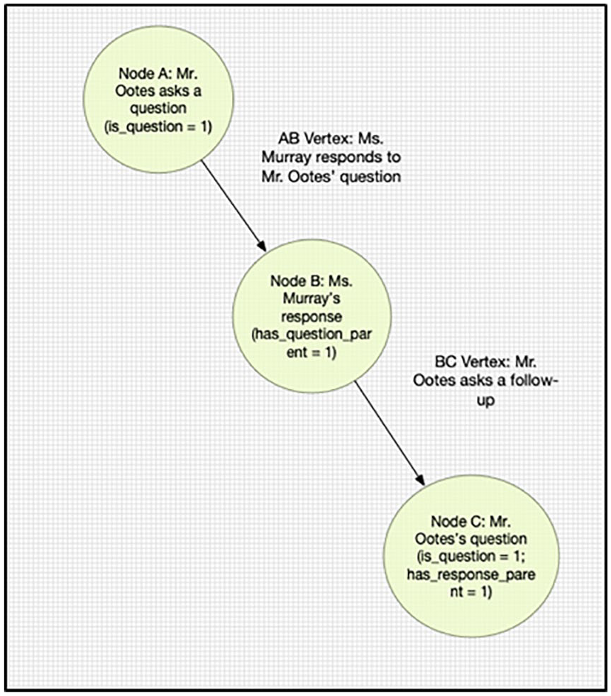
Parliamentary speeches in graph structure.
Coding of speech acts as graph structure.

Vocabulary-based features
Over time, we developed lists of terms that could be indicative of a certain indicator class, but which by themselves, would not accurately predict the class of hundreds of thousands of speech acts. We inserted vocabularies into the TF-IDF matrices developed using words and ngrams, giving them a higher weighting. This was particularly useful on indicators, such as advocacy and public interest, where a manual coder might be looking for specific terms. In the case of the advocacy indicator—which measures whether a speech act explicitly defends or advances the interests or claims of identifiable groups or communities—these terms included unemployed, youth, homeless, constituents, and victims.
Finally, there were circumstances in which it was obvious that a manually pre-selected feature would work best. For example, we stripped punctuation before implementing the above methodologies. In the case of the question indicator, however, it was clear that the presence of a question mark should be manually added in the feature list. The vocabulary for the question classifier therefore only contained one “term,” the question mark.
Character count
In Fournier-Tombs and Di Marzo Serugendo’s (2020) previous work, character count is one of the most important features used to determine discourse quality. In their analysis, longer blog posts typically attained a higher DQI score than shorter ones. This finding is consistent with other studies, such as Blumenstock’s (2008) discovery that the length of a Wikipedia article is an accurate predictor of quality. In our analyses, we therefore added character count as a feature to many of our classifiers, not only to increase accuracy but also to explore any correlations between our deliberative quality indicators (such as narrative) and the length of speech acts. In addition, we used a categorization of word counts, using a statistically determined “low,” “medium,” and “high” word counts, which we found to be relevant in several instances.
Summary of feature construction
The current state of supervised machine learning allowed us to use most of the above techniques while allowing the trained model to select the most relevant features for accurate prediction for each indicator.
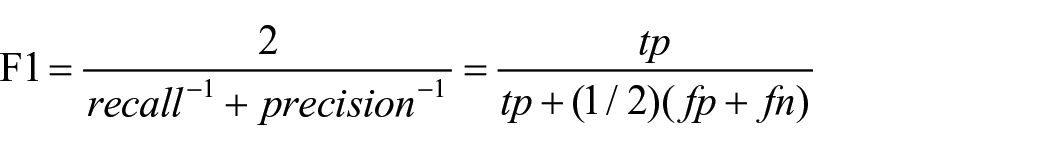
As illustrated below, for each classifier, we set a maximum feature number n. This allowed us to select the most relevant features based on the importance score. Unless there was a strong reason not to do so (as in the case of the question indicator, which we will describe below), we drew features from all of the feature classes. For a given model, the top feature could be character count, the second one might be the word “country,” the third one might be a part-of-speech, the fourth might be another word, and so on. To measure the accuracy of the models once they were trained, we used the F1 score. The F1 score is an accepted best-practice used in machine learning classification. It consists of the harmonic mean of precision and recall, two metrics which measure the proportion of false positives and false negatives
In this demonstration, we set the feature number cut-off to 500. We found that after 500, there were no advantages in including additional features in the model, and leaving too many features in the model tended to slow down the runtime. In Table 6, we show the trade-off between runtime and accuracy. The difference in runtime is not significant in our case, 4 but might make a difference when running on slower systems or much larger datasets.
Demonstration of script runtime and model accuracy by feature count for Yukon narrative classifier (in milliseconds).

Results
The preliminary run using this methodology for all three territories and 12 indicators yielded good results for most, but not all, indicators, some of which required the addition of rule-based techniques. In the examples marked with one asterisk, we faced class imbalance, which meant that the vast majority of the cases in the training datasets were of the same value. In the examples marked with two asterisks, we found that the random forests model was improperly conducting feature selection, due to the very small number of predictive variables (Tables 7 and 8). The solutions to these two problems will be discussed in the “Case studies: coding for narrative, constructive proposal, response, question, and respect” section. Once the modifications were applied, the accuracy of the models improved considerably.
Accuracy of models using machine learning techniques only.

NU: Nunavut; NWT: Northwest Territories: YU: Yukon.
Indicator key: [1] interruption 5 ; [2] explanation; [3] causal reasoning; [4] narrative; [5] question; [6] response; [7] advocacy; [8] public interest; [9] disrespect; [10] respect; [11] counterarguments; [12] constructive proposal.
Accuracy of models using machine learning and rule-based techniques.

NU: Nunavut; NWT: Northwest Territories: YU: Yukon.
Indicator key: [1] interruption 5 ; [2] explanation; [3] causal reasoning; [4] narrative; [5] question; [6] response; [7] advocacy; [8] public interest; [9] disrespect; [10] respect; [11] counterarguments; [12] constructive proposal.
Case studies: coding for narrative, constructive proposal, response, question, and respect
In the following section, we discuss in more detail some of the indicators that yielded the best results with the machine learning models (narrative and constructive proposal), one that varied by territory (response), and those that performed better with a rules-based approach (question and respect).
Narrative
The narrative indicator acknowledges that speakers often explain themselves, or justify their claims or values, by telling stories or personal anecdotes. The following excerpt from a speech in the Nunavut parliament demonstrates narrative: [. . .] Recently this summer stemming from the spring, my three grandsons were able to hunt and caught their first animal of certain species. I wish to praise their hard work, including every other young person who accomplished this. My grandson is now 13 years old. He shot his first beluga and I took great pride in his first catch. Further, my irngutalluaq, whom I referenced a while back as having caught his first walrus and congratulating him for that accomplishment, just recently caught his first arctic hare on his first solo hunt whilst accompanying his parents on a berry-picking trip. [. . .]
In our analysis, we used all of the feature creation techniques identified above, and allowed the algorithm to select which would be weighted more heavily.
The greatest challenge in correctly identifying narrative was the heterogeneity of the labeled data. Stories are particularly subjective, and they take on many different shapes. However, as illustrated below, certain phrases and parts-of-speech, as well as the length of the speech acts, proved relevant.
To highlight the features used by the classifiers to identify narrative, we produced boxplots, which demonstrate the range of importance scores for each feature class, along with histograms, which illustrate the number of features belonging to each class. The summary statistics are also shown below.
In all three cases, the TF-IDF 2-ngram and the TF-IDF word feature classes figure prominently in the feature lists. Examples from the top 20 features in each territory include the following:
“it was,” “the first,” “the year,” “once” (Nunavut)
“the territory,” “our colleagues,” “lake” (Yukon)
“right,” “elders,” “river” (NWT)
Although the classifiers do not use individual features as much as a combination of features to determine classes, the phases listed under Nunavut in particular seem to intuitively relate to storytelling (Figures 3 and 4).
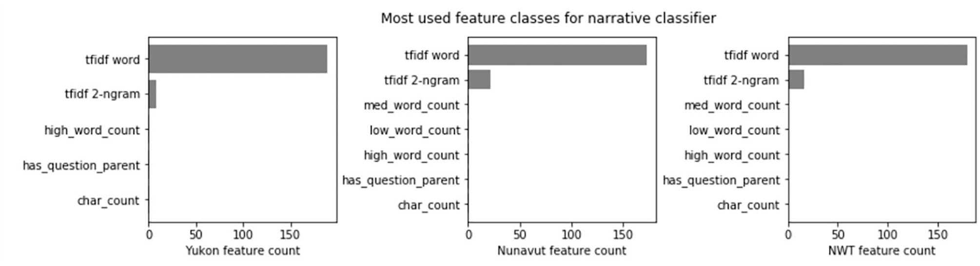
Illustration of most common feature classes for features used in narrative classifier.
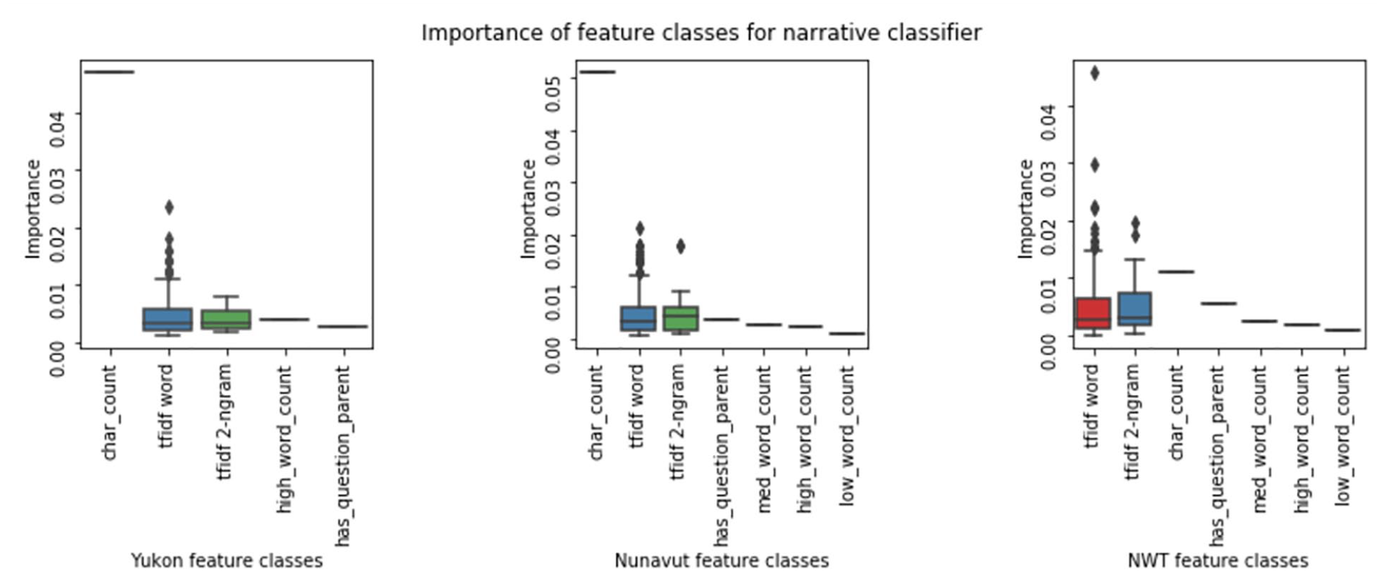
Distribution of feature importance by feature class for narrative classifier.
Interestingly, while character count is the most important feature used by the Yukon and Nunavut classifiers on the narrative indicator, it is much less important in NWT on this indicator. This may be related to particularities in the training dataset; in the case of NWT, the longest speech is not a narrative, whereas the opposite is true of the other territories. As we see in the character count summary statistics in Table 6, overall, however speeches that include narrative in all territories are longer than non-narrative speeches.
Going a step further, we discovered that the difference between narrative and no-narrative samples is highly statistically significant in all three cases (the p-value between the two treatments is less than 0.0001). However, the lesser importance of character count in the NWT case is likely due instead to the precedence of other important features.
It is also worth noting that when it comes to predicting narrative, the other feature classes are rarely used by the classifiers, with the exception, in Nunavut, of a single part-of-speech feature, “IN,” which is a “preposition, subordinating conjunction” such as “in,” “of” or “like.” As seen in Table 9, the accuracy scores for the narrative indicator were 0.95 for NWT, 0.87 for Nunavut, and 0.78 for the Yukon.
Distribution of character count in no-narrative and narrative samples in Nunavut, Yukon, and Northwest Territories.

Constructive proposal
The constructive proposal indicator is used when speakers suggest solutions to shared problems, alternative options, or compromises. In this example from the NWT, a representative listens to a Minister’s response and makes the following suggestion: Maybe if the Minister really wants to get it, maybe they can have a program for communities like Aklavik, to ensure that we have a shoreline erosion program that is there for communities that are along the shoreline of the river systems and in regards to lakes and whatnot. So when we see this erosion taking place, we actually have a program out there that people can access public funds to shore up their communities so that they are in the future.
The models built for all three territories used all of the features identified, with the addition of a vocabulary. The vocabulary allowed for a higher TF-IDF weighting of certain words identified by the research team. This technique was useful in particular because there were few examples of constructive proposals in the data, as they would typically come after several arguments had been made. In the case of constructive proposals, building a vocabulary list considerably improved the true positive rate, which would have otherwise necessitated a much larger training dataset (Figures 5 and 6).
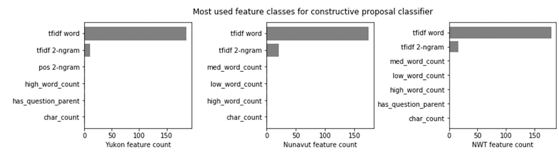
Illustration of most common feature classes for features used in constructive proposal classifier.
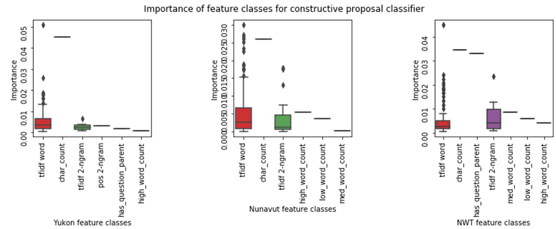
Distribution of feature importance by feature class for constructive proposal classifier.
All three models shared the same vocabulary, which included terms such as suggest, propose, alterative, can we, have we, my idea, we could, and one option. With this technique, we achieved accuracy scores of 0.81 for NWT, 0.94 for Nunavut and 0.92 for Yukon.
Question
The question indicator specifies whether the speaker asks questions of others, which is an important signal that participants in a deliberation are engaging with each other and eliciting the input of others. In the classification of this indicator, we used the vocabulary-based approach, which in this case contained only one “term”—the question mark. In the labeled dataset, there are a few questions that do not have a question mark, particularly in the NWT—these are currently being ignored by the models.
The question indicator has the particular characteristic of being heavily reliant on one feature. When we used the 500-feature set to train the classifiers, we found that their accuracy was much lower than if we only used one feature. The other features in effect created confusion and were best removed completely. Table 10 shows the contrast between the accuracy of the classifiers using all features and the classifiers using only the question mark feature. This shows that unless there are many speeches in the dataset that have questions without a question mark, the other possible features should be ignored.
Comparison of question model accuracy by feature count for Nunavut, Yukon, and NWT.

As shown in Table 9, the question indicator achieved high accuracy scores using this method in Nunavut (0.95) and Yukon (0.92). The accuracy score for this indicator was lower in NWT (0.75) because there was a period of time when the data did not include question marks.
Response
The response indicator specifies whether those who are asked questions answer them instead of avoiding them or speaking only about their own interests or concerns. The following is the response given to the question that was asked in the previous example (see p. 13): Thank you, Mr. Speaker. It’s my understanding that there are five vacant positions in Pond Inlet right now and they are for four project managers and one facility manager. That is my understanding of the current situation there. Thank you.
As we did when training the algorithm to predict the narrative indicator, in this case we started by using all of the feature creation techniques described in the section above. We expected the algorithm to use the structural features of the deliberation in its predictions because responses would often be “child” nodes to “parent” nodes, such as questions. In this case, the classifiers weighted the features according to the following feature classes (Figures 7 and 8).

Illustration of most common feature classes for features used in response classifier.
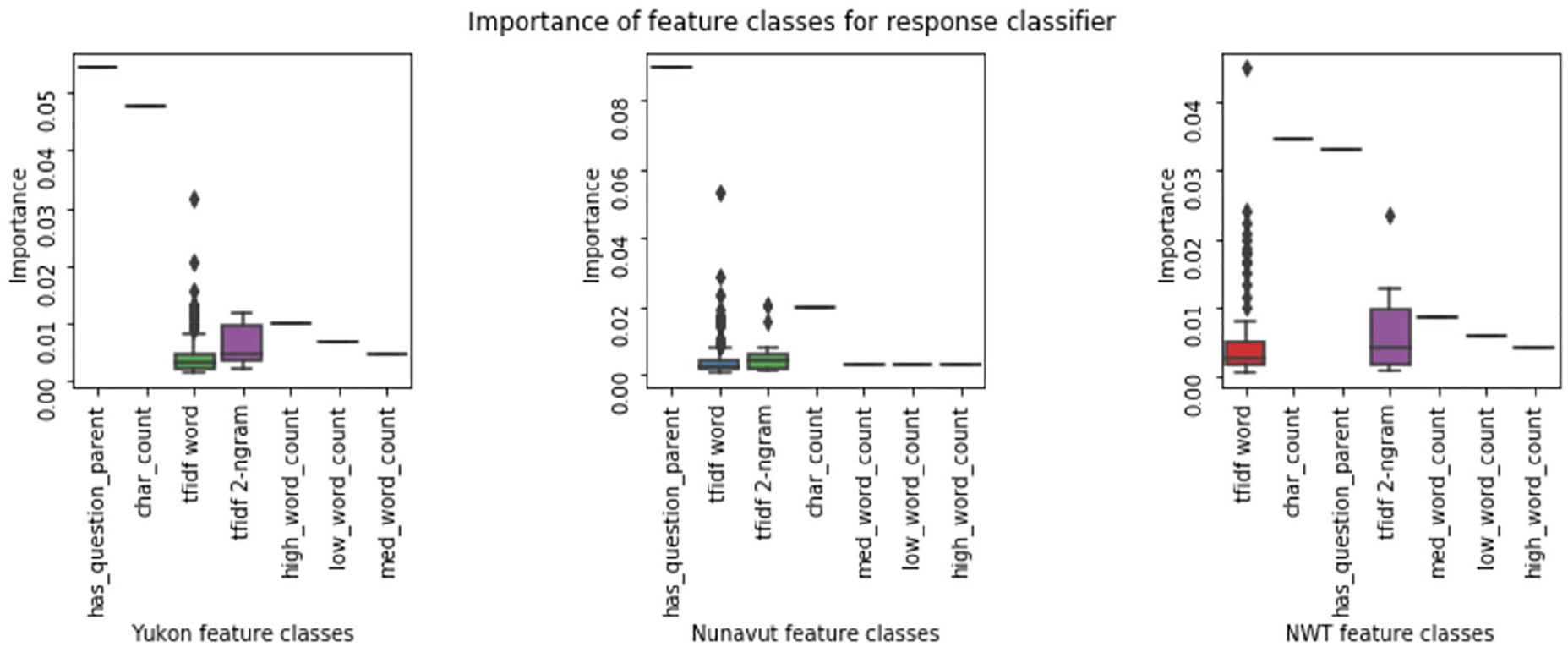
Distribution of feature importance by feature class for response classifier.
In addition to the expected TF-IDF feature classes, a prominent feature is has question parent, which verifies if the previous speech is a question. This is particularly the case in the Nunavut and the Yukon classifiers, where this feature is the most important one. The character count feature is important in the NWT, as well as the TF-IDF word feature class, which includes terms such as “residents,” “programs,” “responsible,” and “question”—as in “thank you for your question.” Interestingly, in two of the territories, we observe that responses in the labeled dataset are shorter than the average speech. We might have expected that responses might require more time than questions. However, we often observe a preamble and even a narrative in the questions, which helps explains their length. The accuracy score for the response indicator was 0.83 for NWT, 0.72 for Nunavut, and 0.77 for Yukon (Table 11) .
Distribution of character count in no-response and response samples in Nunavut, Yukon, and NWT.

Respect
Our fourth example is the respect indicator. Respect indicates statements which include explicit shows of respect, such as salutations, complements, or apologies. Below is an example from the Yukon parliament: I do appreciate the positive words from the Education minister, but I think that time is of the essence. [. . .]
Just like the question classifiers, the respect classifiers perform better when using a manually selected feature—in this case the presence of a word from a respect vocabulary. These classifiers were therefore trained only on the vocabularies, in a manner similar to positive and negative words vocabularies used in sentiment analysis. Examples of respect phrases included “thank you,” “welcome,” and “I apologize.” As can be seen in Table 12, the accuracy scores for the respect indicator were often quite low when the program used all features—notably in Nunavut and NWT—but were high when the vocabulary was used. As with the question indicator, additional features classifications appear to have introduced confusion as opposed to clarity.
Comparison of respect model accuracy by feature count for Nunavut, Yukon, and Northwest Territories.

Summary of methods
In the previous sections, we discussed the vectorization techniques used to model four indicators in each of the three territories. In Table 13, we summarize the techniques selected for all 12 of the indicators in the DQI 2.0.
Summary of vectorization techniques.

TF-IDF: term frequency-inverse document frequency.
In this section, we further discussed five representative indicators. The respect and constructive proposal indicator models demonstrated vectorization using a vocabulary, in slightly different ways. Vocabulary-based vectorization can also be used when identifying mentions in a text—of names, entities, or topics (e.g. a politician or a policy issue). The question indicator model also demonstrated vocabulary-based vectorization using a very obvious character: the question mark. Models with similar characteristics might include the mention of budget items (dollar signs and numbers) or calculating gender balance in discussions using gender-specific titles such as Ms. or Mr. The response indicator model highlighted a vectorization technique that contained both ngram and graph features. Similar models, in which the order of the texts prove to be relevant, might include those concerned with finding an information moderator or influencer, or tracking the contagion of ideas. Finally, the narrative indicator model showed a vectorization technique for models in which there might be various syntactic or vocabulary constructs that are not immediately obvious to the researcher.
Conclusion
In this article, we have presented a methodology for the development of machine learning models to measure the 12 indicators in the DQI 2.0. We focused on vectorization techniques in particular—transforming the texts into data for model training. We showed that the vectorization techniques used were flexible, allowing for the observation of narrative, question, response, and respect in speech. This research is a critical component of a larger research project that will use these techniques to model each of the 12 indicators in the DQI 2.0 for three legislatures—Nunavut, NWT, and Yukon—over 20 years. Without the techniques described here, it would not be possible to conduct such a comprehensive study, due to the sheer volume of data. The purpose of this article was to provide detailed illustrations of the methodologies we have developed so that they might be used by other social scientists and communications scholars.
The main challenge that we sought to address in this article was the issue of appropriate vectorization. Using machine learning to measure deliberative quality has, however, other challenges that we have not addressed. First, we continue to be reliant on high quality training data, which must be manually coded. Having considered this issue, we propose that having a training dataset is akin to having a “guiding hand” of trained political analysts applying the appropriate coding to each situation. We therefore have not ascertained whether using unsupervised learning techniques or manually selecting features in each case (as we do for the question indicator) would be more desirable. Second, our ability to train the algorithm to accurately predict each indicator also depends on the quality of the source dataset. Our datasets contain large individual speech acts, and they possess a certain homogeneity of style within each territory. With shorter and more heterogenous speech acts, it might be more difficult for machine learning models to select the appropriate features and weights.
Nevertheless, there are many other possible applications for the machine learning models and vectorization techniques that we describe in this article. Although the DQI (Steenbergen et al., 2003) was originally developed to analyze parliamentary speeches, it has been used in other fora such as minipublics (Marcus et al., 1993), deliberative blogs, and social media (Fournier-Tombs and Di Marzo Serugendo, 2020). Similarly, our machine learning methodology could be applicable to any deliberative space, online or offline, or used to conduct systematic comparative analyses of other textual data such as media debates, political speeches, and legislation. It is our hope that this methodology will enable researchers to more effectively analyze deliberative quality—and many other features of political communication more generally—using large (or very large) datasets.
Footnotes
Declaration of conflicting interests
The author(s) declared no potential conflicts of interest with respect to the research, authorship, and/or publication of this article.
Funding
The author(s) received no financial support for the research, authorship, and/or publication of this article.