Sage Journals: Discover world-class research

Abstract

Model-data fit indices for raters provide insight into the degree to which raters demonstrate psychometric properties defined as useful within a measurement framework. Fit statistics for raters are particularly relevant within frameworks based on invariant measurement, such as Rasch measurement theory and Mokken scale analysis. A simple approach to examining invariance is to examine assessment data for evidence of Guttman errors. I used real and simulated data to illustrate and explore a nonparametric procedure for evaluating rater errors based on Guttman errors and to examine the alignment between Guttman errors and other indices of rater fit. The results suggested that researchers and practitioners can use summaries of Guttman errors to identify raters who exhibit misfit. Furthermore, results from the comparisons between summaries of Guttman errors and parametric fit statistics suggested that both approaches detect similar problematic measurement characteristics. Specifically, raters who exhibit many Guttman errors tended to have higher-than-expected Outfit MSE statistics and lower-than-expected estimated slope statistics. I discuss implications of these results as they relate to research and practice for rater-mediated assessments.

Keywords

Guttman scaling invariant measurement model-data fit nonparametric performance assessment rater effects rating scales

The purpose of this article is to present and illustrate an approach that researchers and practitioners can use to evaluate the quality of raters’ ratings in rater-mediated performance assessments, such as writing assessments in which raters score students’ compositions, or teacher evaluations in which principals conduct classroom observations and rate teachers’ effectiveness. Most often, researchers who study rater-mediated performance assessments use group-level rater reliability statistics, such as Cohen’s kappa coefficient (Cohen, 1968) and rater agreement statistics to evaluate ratings (Wind and Peterson, 2017). Although evidence of rater reliability is important, these coefficients provide somewhat limited information about individual raters. Specifically, rater consistency statistics such as kappa provide researchers and practitioners with evidence of the degree to which a group of raters consistently rank-orders examinee performances (reliability statistics) or evidence of the degree to which raters provide matching ratings on the same performances (agreement statistics). This approach does not provide insight into the degree to which raters’ interpretations of examinee performances conform to any measurement theory (e.g. invariant measurement) or theories about the construct measured by the performance assessment. Furthermore, these statistics provide limited diagnostic information about rating quality at the individual rater level. Specifically, statistics such as kappa do not provide information about individual raters’ rating scale category use, systematic biases related to test-taker characteristics, or other rater effects.

As a more theoretically driven alternative to rater consistency and agreement statistics, many researchers have proposed methods for evaluating rating quality based on item response theory (IRT) models. Such analyses provide a variety of indicators of rating quality, such as the degree to which raters exhibit different overall levels of severity exhibit consistent levels of severity over different subgroups of examinees and interpret rating scale categories as intended. Particularly in contexts where rater judgments have notable consequences, this information is critical for evaluating the fairness of rater-mediated assessments. Most importantly, rating quality indices based on IRT allow researchers and practitioners to evaluate rating quality within clear theoretical frameworks based on expected measurement properties. Specifically, IRT analyses incorporate model-data fit analyses. Essentially, researchers conduct model-data fit analyses to evaluate the degree to which their data reflect the expected characteristics according to the model that they have chosen. When researchers use models with strict requirements, they can use model-data fit analyses to identify raters, items, students, or other aspects of the assessment system that do not adhere to expectations and thus warrant additional investigation.

When researchers apply IRT models to rater-mediated performance assessments, they often calculate model-data fit indices for individual raters (i.e. rater fit statistics) as a method for evaluating the quality of raters’ ratings (e.g. Engelhard and Wind, 2018; Myford and Wolfe, 2004; Wolfe and McVay, 2012). These rater fit statistics provide insight into the degree to which individual raters’ judgments reflect what is considered appropriate according to a particular model. For example, when they are applied to raters, models based on Rasch measurement theory (Rasch, 1960) require that raters exhibit consistent severity for all examinees and that judgments of examinee achievement are consistent over all raters (i.e. invariant measurement; Engelhard and Wind, 2018). Briefly, Rasch measurement theory models are parametric IRT models that use a logistic function to transform raters’ ordinal ratings (i.e. ratings in a series of ordered rating scale categories) to a linear scale on which rater severity and examinee achievement levels can be estimated. Like other parametric IRT models, the logistic transformation used in Rasch analyses imposes a specific mathematical form (the logistic ogive) of the rater response function (RRF), or the probabilistic relationship between expected ratings from each rater and examinee achievement. Furthermore, Rasch models require that all RRFs exhibit equal slopes (i.e. discrimination), such that raters can be ordered consistently by severity for all examinees. Likewise, examinees must have a consistent ordering over all raters. Together, these properties allow researchers and practitioners to evaluate rating quality within a strong framework based on invariance.

Researchers who apply Rasch models to rater-mediated assessments have proposed numerous techniques for evaluating invariance in rater-mediated assessments. Because the framework clearly specifies requirements for raters and examinees, researchers actively seek to identify violations of invariance in order to improve the quality of rater-mediated assessments. For example, popular rater fit indicators within the framework of Rasch measurement theory include numeric summaries of the residuals associated with individual raters (Engelhard and Wind, 2018; Myford and Wolfe, 2004), and indicators of individual raters’ discrimination among test-takers with low and high achievement (i.e. rater slope; Schumacker, 2015; Wind et al., 2016; Wolfe, 1998). When researchers use these numeric fit indicators, they compare the value of fit statistics to the value that would be expected if the responses exactly matched the requirements of the Rasch model. Additionally, several researchers have used graphical displays to explore rater fit, including plots that highlight the difference between observed and expected ratings for individual raters (Kaliski et al., 2013; Wind and Schumacker, 2017).

Nonparametric IRT methods for evaluating rater fit

Several researchers (Junker and Sijtsma, 2001; Meijer and Baneke, 2004; Molenaar, 2001; Santor and Ramsay, 1998) have observed that, although it is possible to use parametric IRT models to estimate examinee achievement and item difficulty, the logistic transformation employed by these models is not always appropriate. Specifically, when one applies a parametric IRT model to response data, the estimates of item difficulty, examinee achievement, and other parameters depend on a number of strong assumptions. Importantly, the estimates depend on the assumption that a logistic ogive is an accurate representation of the probabilistic relationship between examinee achievement and item difficulty (or in this case, rater severity) and that the sample is large enough to produce precise parameter estimates that hold for the entire sample. When these assumptions are not met, estimates from parametric IRT models are difficult to interpret, imprecise, and unlikely to hold over replications. For example, Reise and Waller (2003) demonstrated the consequences of inappropriately applying several parametric IRT models to data in which item responses did not exhibit a logistic structure. They found that multiple models “fit” in a global model-data fit evaluation, but that the parameter estimates reflected artifacts of the models. In other words, the models did not provide an accurate summary of the characteristics of the data. Along the same lines, the requirement for a logistic structure can potentially lead researchers to discard items (or raters) for which there are violations of model assumptions within certain ranges of examinee achievement, but that exhibit productive measurement properties in other ranges of achievement—this is particularly likely with small samples (Meijer and Baneke, 2004; Santor and Ramsay, 1998). As Molenaar (2001) observed, “there remains a gap … between the organized world of a mathematical measurement model and the messy world of real people reacting to a real set of items” (p. 295). This “messiness” is certainly present, and perhaps even more acute, in the context of raters using rating scales to evaluate examinee performances.

It is possible to use a nonparametric approach to examine rater fit from the perspective of invariant measurement. Nonparametric methods based on invariant measurement are promising in the context of rater-mediated assessments because they do not involve potentially inappropriate transformations of ordinal ratings, but still provide a strong theoretical framework and diagnostic indices in which to evaluate rating quality. Furthermore, nonparametric IRT models can be used in situations where parametric models may not be appropriate, such as when there are a small number of raters or test-takers, as is often the case during rater-training programs or in small-scale assessments. This approach is also useful when information about raters’ and examinees’ relative ordering is sufficient to inform decisions, and it is not necessary to use interval estimates that would be obtained from a parametric IRT model. Because these models are less restrictive than parametric IRT models, Meijer and Baneke (2004) observed that they provide “information about the quality of the data without forcing the data to conform to a logistic IRT model” (p. 360).

A simple nonparametric approach to examining invariance is checking for Guttman errors. Essentially, Guttman errors are instances of an incorrect response on an easy item paired with a correct response on a more-difficult item (described further later in the article). In previous studies, researchers have recognized Guttman errors as useful fit statistics in a variety of contexts, including item fit (Mokken, 1971) and person fit (Meijer, 1994). Furthermore, Guttman errors form the basis for the scalability coefficients that are used as model-data fit statistics in Mokken scale analysis (MSA), which is a nonparametric approach to IRT (Sijtsma and Molenaar, 2002).

MSA scalability coefficients are available for evaluating both dichotomous responses (i.e. responses in two categories) and polytomous responses (i.e. responses in three or more categories), and many researchers have used these statistics to evaluate the quality of their social science measurement instruments (Freedland et al., 2016; Gillespie et al., 1988; Muncer and Speak, 2016; Paas, 1999; Van der Veer et al., 2011). In this study, I considered the use of scalability coefficients as a method for evaluating rater fit in rater-mediated performance assessments within the framework of invariant measurement.

Purpose

The purpose of this study is to consider a nonparametric approach to evaluating rater fit based on Guttman errors. I used scalability coefficients calculated based on an adaptation of MSA (Wind, 2016) to summarize Guttman errors for raters, and I considered the alignment between rater scalability and parametric IRT indicators of rater fit. I focused on the following research questions:

How can researchers use Guttman errors to explore rater fit?

How do summaries of raters’ Guttman errors correspond to parametric IRT model indicators of rater fit?

How do summaries of raters’ Guttman errors correspond to graphical displays of rater fit?

Scalability coefficients

When he presented his nonparametric approach to IRT, Mokken (1971) proposed scalability coefficients as statistics that researchers and practitioners can use to gauge the psychometric quality of items in terms of their contribution to a scale. Scalability coefficients are calculated using frequencies of Guttman errors. As noted previously, Guttman errors occur when incorrect responses to easier items are found in combination with correct responses to more-difficult items. Figure 1 illustrates Guttman errors for dichotomous items using three example items (Item i, Item j, and Item k). The item difficulty ordering (Item i < Item j < Item k) is used to define Guttman errors. Each cell entry includes an examinee’s response to an item, where “1” indicates a correct response and “0” indicates an incorrect response. Panel (a) includes no Guttman errors, because the item responses proceed from correct to incorrect as the items proceed from easy to difficult and as examinee achievement increases from low to high. Panel (b) includes two Guttman errors, each of which is marked with italics and an asterisk. Guttman errors occur when a score of “1” appears to the right of a score of “0.” Researchers generally consider Guttman errors problematic because they imply that the difficulty ordering of the items is not the same for all of the examinees. One can use the ratio of observed-to-expected Guttman errors to calculate scalability for pairs of items, individual items, and a set of two or more items. Values of scalability coefficients reflect the influence of Guttman errors on the quality of a measurement procedure, where fewer Guttman errors correspond to higher scalability coefficients and frequent Guttman errors correspond to lower scalability coefficients.

Figure 1.

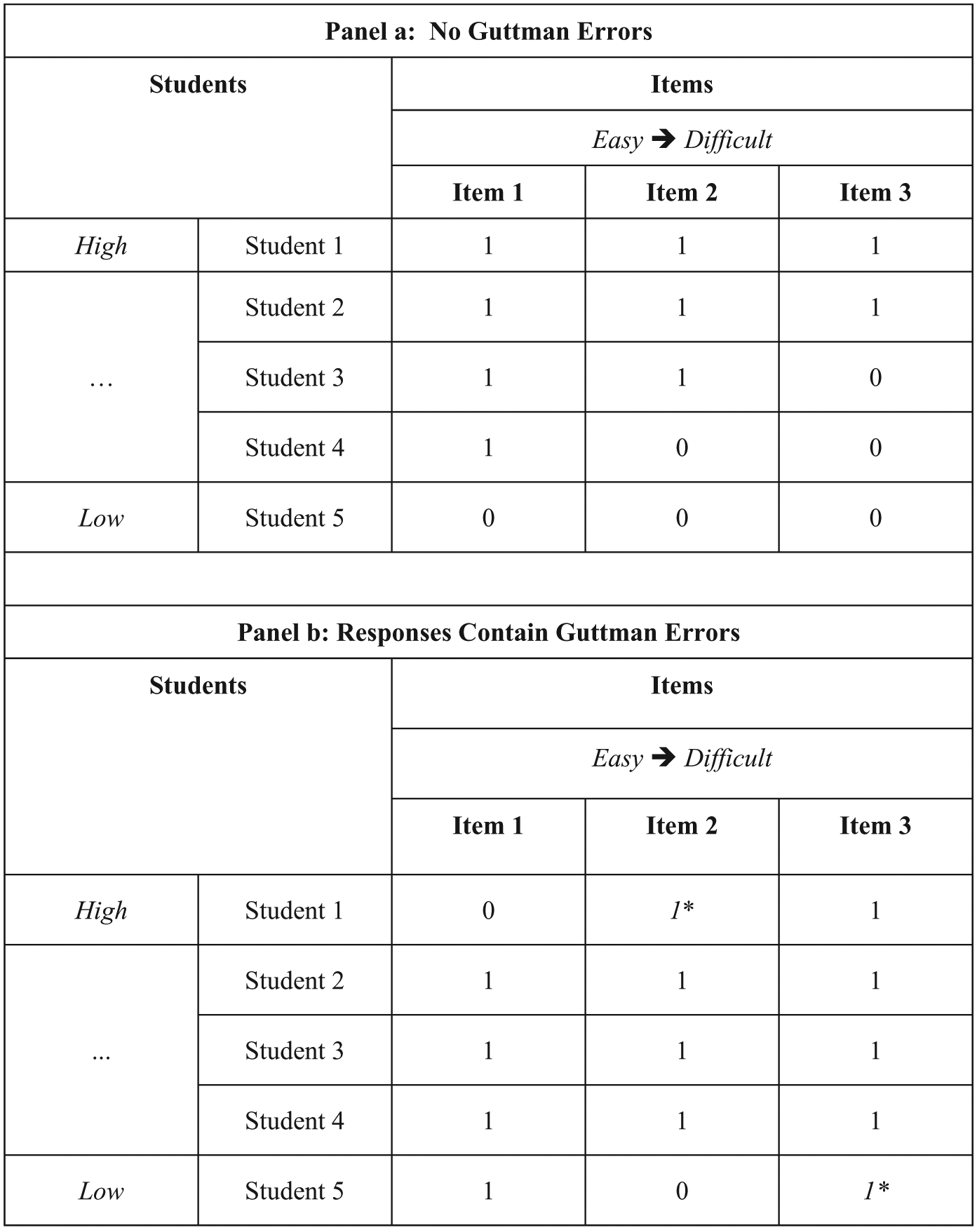
Illustration of Guttman errors for dichotomous items.

Polytomous scalability coefficients

Molenaar (1982) presented polytomous versions of Mokken’s (1971) scalability coefficients for evaluating item responses in three or more categories. To evaluate scalability when items include more than two categories, it is necessary to adjust the procedure for defining Guttman errors from the procedure used for dichotomous items. Specifically, it is necessary to consider polytomous items as a set of dichotomous “items” or thresholds between rating scale categories. For example, if an item had a four-category rating scale (0, 1, 2, 3), there would be three thresholds: (1) between category 0 and 1, (2) between category 1 and 2, and (3) between category 2 and 3. Then, instead of ordering items overall as in the dichotomous case, one can use the proportion of ratings in each item-category combination to identify Guttman errors. As Molenaar (1982) noted, one can identify the frequency of Guttman errors within pairs of polytomous items as the frequency of responses in which a person has “passed a certain item step but failed an easier one” (p. 124). In a similar fashion, it is also possible to identify Guttman errors for individual raters who rate student performances using a polytomous rating scale. Similar to the approach that many researchers have used to model raters using parametric IRT models (Eckes, 2015; Myford and Wolfe, 2004; Wolfe and McVay, 2012), one can treat raters as a type of item or “assessment opportunity” and evaluate raters’ measurement characteristics using nonparametric analyses such as MSA (Mokken, 1971).

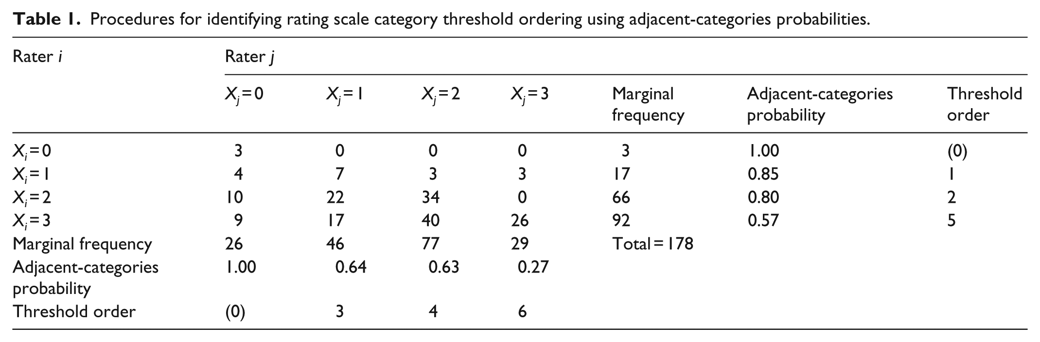
Recently, Wind (2016) presented an alternative approach to polytomous MSA in which rating scale category thresholds are calculated as the probability for a rating in a particular category, rather than the category just below it. As a result, this adjacent-categories MSA (ac-MSA) approach is different from traditional polytomous MSA analyses (Molenaar, 1982, 1997), and it is more closely aligned with the way in which researchers and practitioners interpret rating scale categories in educational performance assessments (for details, please see Wind, 2016). Table 1 illustrates the procedure for identifying the empirical difficulty ordering of rating scale category thresholds using adjacent-categories probabilities. In the illustration, two raters (Rater i and Rater j) rated a set of 178 performances using a 4-category rating scale (0, 1, 2, 3). The marginal frequencies are either the row total (Rater i) or column total (Rater j). Adjacent-categories probabilities are calculated such that the probability is the observed frequency of ratings in category k or higher, divided by the frequency of ratings in category k and k − 1. For example, the probability for a rating in category 1 from Rater i is the marginal frequency for a rating in category 1 from Rater i divided by the total frequency of responses in category 0 and 1 for Rater i (17/(3 + 17) = 0.85). Using adjacent-categories probabilities, one can identify the expected threshold ordering using the probabilities, ordered from high to low. Excluding the first category (category 0, probability = 1.00), the threshold ordering is as follows: X_i = 1; X_i = 2; X_j = 1; X_j = 2; X_i = 3; X_j = 3. Violations of this ordering constitute Guttman errors.

Table 1.

Procedures for identifying rating scale category threshold ordering using adjacent-categories probabilities.

Rater i	Rater j
Rater i	X_j = 0	X_j = 1	X_j = 2	X_j = 3	Marginal frequency	Adjacent-categories probability	Threshold order
X_i = 0	3	0	0	0	3	1.00	(0)
X_i = 1	4	7	3	3	17	0.85	1
X_i = 2	10	22	34	0	66	0.80	2
X_i = 3	9	17	40	26	92	0.57	5
Marginal frequency	26	46	77	29	Total = 178
Adjacent-categories probability	1.00	0.64	0.63	0.27
Threshold order	(0)	3	4	6

Using the illustrative data from Table 1, Figure 2 illustrates the procedure for using the adjacent-categories threshold ordering to identify Guttman errors. First, Panel (a) (top of Figure 2) shows the expected pattern of ratings from Rater i and Rater j. Each cell shows the joint rating from Rater i and Rater j as: (Rater i’s rating, Rater j’s rating). Bold, underlined cells show the expected response pattern given the rating scale category difficulties (see Table 1). Arrows indicate the expected order of ratings from the two raters as examinee achievement moves from low to high. Italicized cells with asterisks indicate deviations from the expected order, which are Guttman errors. Next, Panel (b) (middle section of Figure 2) shows ratings recoded into dichotomous variables (i.e. “steps”) for the expected ratings. In each cell, a “1” indicates passing a threshold, and a “0” indicates not passing a threshold. The sum of scores on these dichotomous threshold variables equals the observed rating. Shading is used to highlight the Guttman-expected pattern of ones systematically transitioning to zeroes from left to right in the matrix. Finally, Panel (c) (bottom section of Figure 2) shows recoded responses for the ratings that include Guttman errors. Guttman errors occur when a “1” appears to the right of a “0”; these patterns are highlighted using italics and asterisks.

Figure 2.

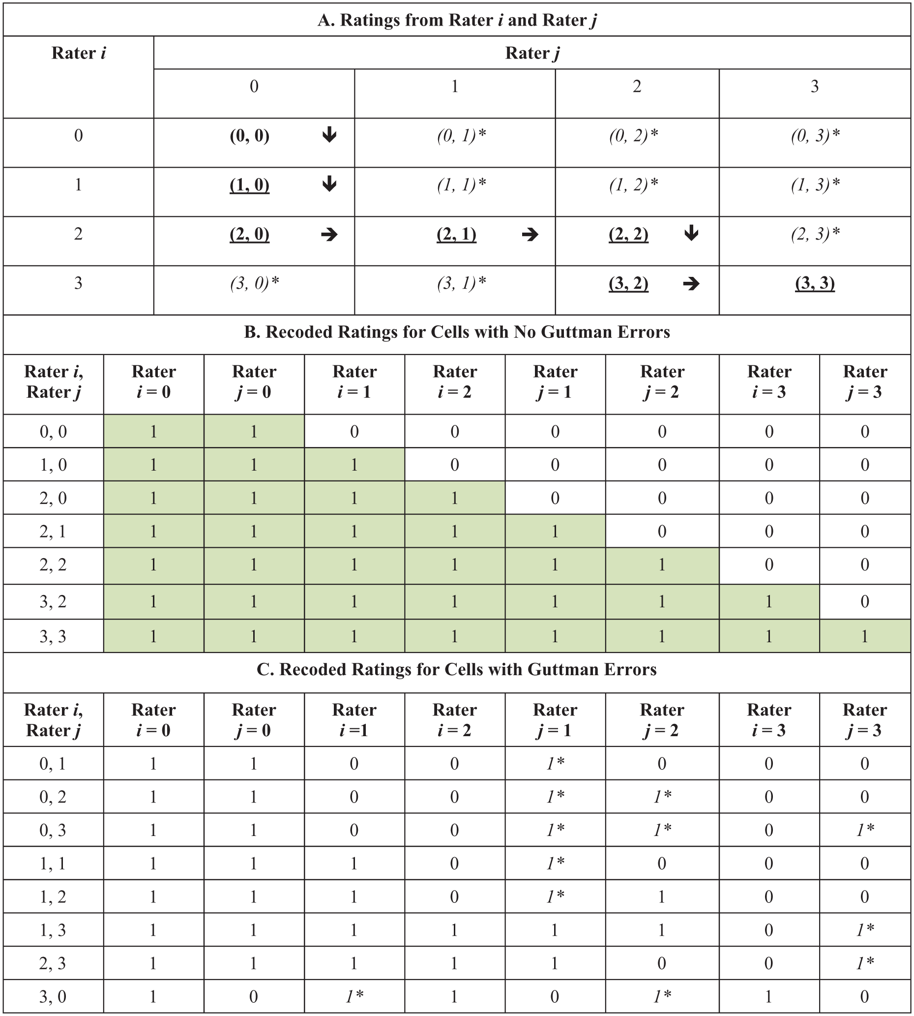
Procedure for using adjacent-categories threshold ordering to identify Guttman errors.

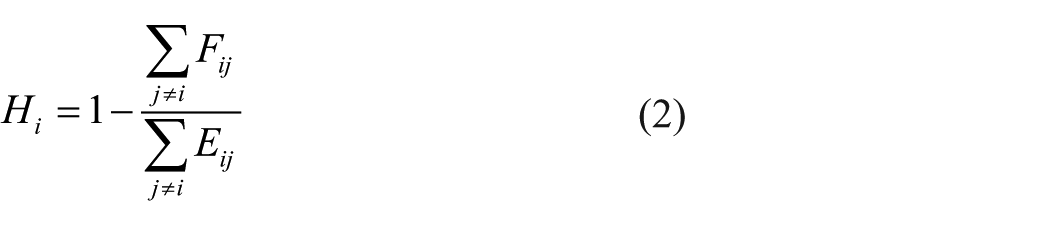
One can then use this observed frequency of Guttman errors, along with the frequency of Guttman errors that is expected given marginal independence, to calculate the scalability of a pair of raters i and j as follows

H_{i j} = 1 - \frac{F_{i j}}{E_{i j}}

(1)

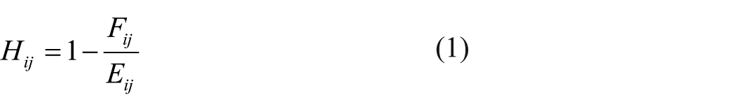
where F_ij is the observed frequency of Guttman errors, and E_ij is the expected frequency of Guttman errors.¹ One can calculate scalability for individual raters using the combination of each rater (i) with every other rater (i ≠ j) as

H_{i} = 1 - \frac{\sum_{j \neq i} F_{i j}}{\sum_{j \neq i} E_{i j}}

(2)

Methods

I used real data from a rater-mediated writing assessment and simulated data to address the research questions for this study.

Real data

The real data were collected during an administration of a statewide high school writing assessment in the United States during which additional ratings were collected for rater calibration purposes. The writing assessment included four extended constructed response (ECR) items for which examinees were required to compose brief expository essays in response to a prompt. In this study, I analyzed ratings of examinees’ responses to one ECR item for which raters rated examinee compositions using a 4-category rating scale (1 = low to 4 = high, recoded to 0 = low to 3 = high prior to analyses). Specifically, I used a subset of data from this writing assessment that included 62 raters’ ratings of 610 examinees’ compositions. As part of the rater calibration procedure, all of the raters rated all 610 of the compositions written in response to the ECR item, such that the rating design was fully crossed (Engelhard, 1997).

Quasi-simulated real data

In order to better understand the generalizability of my results to a wide range of performance assessment contexts, I used the real dataset to create four additional “quasi-simulated” datasets with different sample sizes: (1) 30 raters and 300 examinees, (2) 20 raters and 200 examinees, (3) 10 raters and 100 examinees, and (4) 5 raters and 50 examinees. In each quasi-simulated dataset, I used random sampling without replacement to select the raters and examinees from the original dataset.

Simulated data

In addition to the real data analyses, I also simulated data to address my research questions. Using the R software program (R Core Team, 2018), I simulated polytomous, holistic ratings based on the generalized partial credit (GPC) model (Muraki, 1997).

Variables held constant

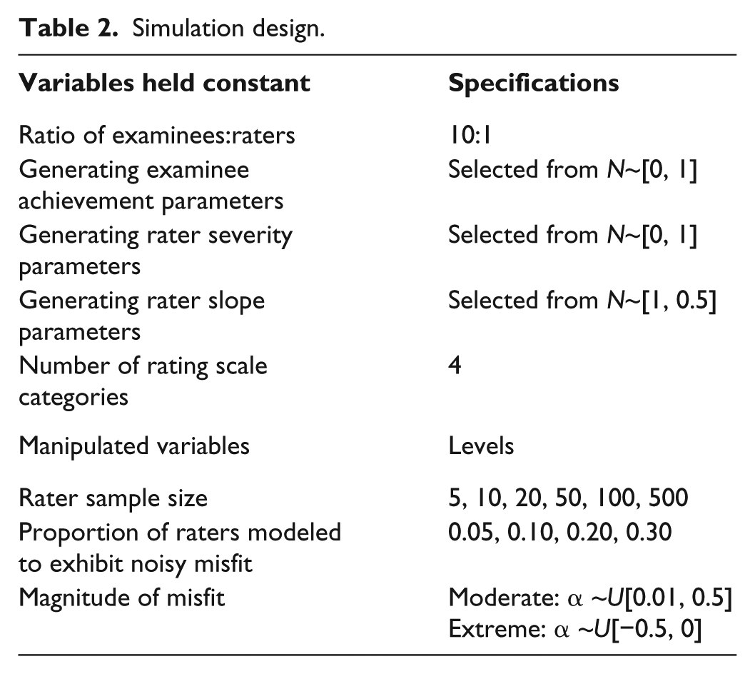
I held several variables constant over each of the conditions in my simulation design (see Table 2). First, I used the same ratio of examinees to raters in all of the simulation conditions. Specifically, I fixed the examinee sample size to 10 times the number of raters in the simulation condition. This ratio of 10 examinees to one rater reflects current practice in educational performance assessments, as well as the sample sizes reported in previous simulation studies of rater-mediated assessments (e.g. Wolfe et al., 2014). Second, following the procedures that researchers have used in previous simulations of rater-mediated performance assessments (e.g. Marais and Andrich, 2011; Wolfe et al., 2014; Wolfe and Song, 2015), I generated examinee achievement parameters and rater severity parameters from a normal distribution with a mean of zero logits and a standard deviation of one logit. Finally, for the raters who I did not model to exhibit misfit, I selected the generating slope parameters for raters from α~N[1.00, 0.05]. I simulated rater slopes to be approximately 1.00 because this is the value that is expected when there is acceptable fit to Rasch models, such as the Rasch Rating Scale model (Andrich, 1978), which is the model that I used as a parametric comparison to the nonparametric rater fit indices (I provide more details about this analysis later in the article). As a result, this procedure resulted in acceptable parametric IRT model-data fit statistics for these raters—providing a frame of reference for interpreting the nonparametric rater fit indices. Finally, I used a rating scale with four categories in all of the simulation conditions. I selected a 4-category rating scale to reflect many recent large-scale performance assessments that are used in the United States, such as the rating scale that is used to score the writing component of the National Assessment of Educational Progress (NAEP; Writing-Achievement Level Details, n.d.), as well as a number of end-of-grade writing assessments (e.g. Commonwealth of Virginia, Department of Education, 2012; Georgia Department of Education, 2015).

Table 2.

Simulation design.

Variables held constant	Specifications
Ratio of examinees:raters	10:1
Generating examinee achievement parameters	Selected from N~[0, 1]
Generating rater severity parameters	Selected from N~[0, 1]
Generating rater slope parameters	Selected from N~[1, 0.5]
Number of rating scale categories	4
Manipulated variables	Levels
Rater sample size	5, 10, 20, 50, 100, 500
Proportion of raters modeled to exhibit noisy misfit	0.05, 0.10, 0.20, 0.30
Magnitude of misfit	Moderate: α ~U[0.01, 0.5]Extreme: α ~U[−0.5, 0]

Manipulated variables

In order to examine rater scalability coefficients under a range of conditions, I manipulated three variables in my simulation study. First, I included six rater sample sizes: 5, 10, 20, 50, 100, and 500 raters. With the ratio of 10 examinees to one rater, these rater sample sizes resulted in examinee sample sizes that ranged from 50 to 5000 examinees. These sample sizes reflect rater-mediated writing assessment contexts that researchers have described in previous analyses of rater-mediated performance assessments (e.g. Brown et al., 2004; Duckor et al., 2014; Raczynski et al., 2015; Wolfe et al., 2010), including the real data used in this study. Second, I incorporated rater misfit into the simulation procedure by modeling four different proportions of randomly selected raters to exhibit misfit (0.05, 0.10, 0.20, or 0.30). Third, I modeled two different magnitudes of misfit: moderate misfit or extreme misfit. To simulate both magnitudes of rater misfit, I selected generating slope parameters for the raters who I modeled to exhibit misfit such that they would be different from the Rasch model-expected value of 1.00. For the moderate misfit conditions, I selected generating rater slope parameters from α ~U[0.01, 0.5]. For the extreme misfit conditions, I selected generating rater slope parameters from α ~U[−0.5, 0.0]. Because the Rasch model expects rater slopes to be equal to 1.00 when data fit the model, I expected these generating slope parameters to result in higher-than-expected fit statistics (i.e. “noisy ratings”; Engelhard, 1994) for the specified raters (Schumacker, 2015). I simulated one hundred unique datasets for each unique combination of the levels of the design factors.

Data analysis

I used a similar procedure to analyze the real, quasi-simulated, and simulated data. First, I calculated scalability coefficients for each rater based on ac-MSA using the procedures described earlier in the article. Second, in order to provide a frame of reference for interpreting the ac-MSA H_i coefficients, I used the Rasch Rating Scale (RS) model (Andrich, 1978) to calculate Rasch Outfit MSE fit statistics for each rater. I calculated Outfit MSE statistics because researchers frequently use this statistic in empirical evaluations of rater fit (e.g. Engelhard and Wind, 2018). Specifically, I used the Facets software program (Linacre, 2015) to calculate Outfit MSE statistics for each rater. Outfit MSE statistics for raters are summaries of residuals, or discrepancies between the ratings that a rater actually gave and the ratings that would have been expected, given their severity estimate. To calculate Outfit MSE, residuals are standardized to a normal distribution. Outfit MSE statistics are calculated as follows

O u t f i t M S E = \frac{\sum_{n}^{N} Z_{n i}^{2}}{N}

(3)

where $Z_{n i}^{2}$ is the squared standardized residual for rater n’s rating of examinee i, and N is the number of examinees.

I also used the Facets software to estimate a slope parameter (i.e. discrimination) for each rater that reflects the degree to which the rater distinguished between examinees with low and high levels of writing achievement. In previous studies, several researchers (Schumacker, 2015; Wind et al., 2016; Wolfe, 1998) have discussed the use of rater slopes as evidence of model-data fit, where slopes that are lower than 1.00 indicate more variation in responses than expected by the Rasch model (i.e. frequent Guttman errors), and slopes that exceed 1.00 indicate less variation than expected (i.e. infrequent Guttman errors).

For the real and quasi-simulated data, I examined values of rater scalability for all 62 raters. For the simulated data, I examined average rater scalability coefficients among the raters who I modeled to exhibit misfit and among the raters who I did not model to exhibit misfit. Then, I calculated the correlation between scalability coefficients and the two parametric indicators of rater fit: Outfit MSE and the estimated slope parameter.

As a final step in my data analysis procedure, I examined graphical displays of rater fit based on ac-MSA. For each rater, I plotted nonparametric RRFs. RRFs are graphical displays that illustrate the relationship between examinee achievement and the probability for a rating in the higher of two adjacent rating scale categories. In ac-MSA, examinee achievement is represented using total scores. However, in order to evaluate individual raters, it is necessary to calculate total scores (i.e. sums of ratings across all of the raters) that do not include ratings from the rater of interest. In MSA, these corrected total scores are called restscores. When RRFs match ac-MSA assumptions, the probability for a rating in the higher of each pair of adjacent rating scale categories is non-decreasing over increasing levels of examinee achievement. Figure 3 illustrates an RRF that shows the expected characteristics based on ac-MSA.

Figure 3.

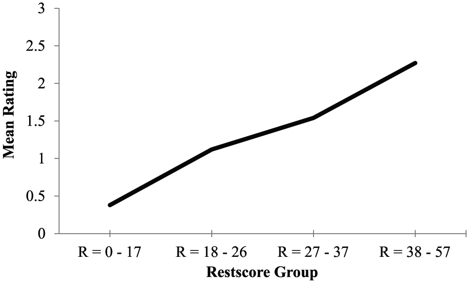
Expected shape of a rater response function when there is acceptable model-data fit to adjacent-categories Mokken scale analysis.

Results

Real data results

Table 3 includes a summary of the rater analyses for the writing assessment data. First, Table 3 includes each rater’s average rating calculated over all 610 examinee compositions, along with rater severity estimates (λ) and standard errors (SE) calculated using the Rating Scale model. Higher average ratings and lower severity estimates indicate that raters were generally lenient (i.e. raters assigned high ratings often), and lower average ratings and higher severity estimates indicate that raters were generally severe (i.e. raters assigned low ratings often). On average, Rater 9 was the most lenient rater (average rating = 2.77, λ = −2.31; SE = 0.09), and Rater 36 was the most severe rater (average rating = 0.44, λ = 2.41; SE = 0.07).

Table 3.

Real data results.

Rater ID	H_i	Average rating	Rasch measure (logits)	SE	Outfit MSE	Estimated slope
1	0.33	2.00	−0.42	0.05	0.93	1.13
2	0.32	2.07	−0.55	0.05	0.90	1.12
3	0.29	2.29	−0.96	0.06	0.98	1.06
4	0.28	2.55	−1.58	0.07	0.96	1.04
5	0.34	1.30	0.67	0.05	0.90	1.13
6	0.24	2.42	−1.24	0.06	0.96	1.02
7	0.20	2.69	−2.04	0.08	0.84	1.07
8	0.34	2.08	−0.57	0.05	0.87	1.19
9	0.28	2.23	−0.84	0.06	1.02	0.96
10	0.10	1.55	0.29	0.05	1.54	0.09
11	0.32	2.30	−0.98	0.06	0.84	1.16
12	0.31	1.00	1.15	0.05	1.01	1.03
13	−0.03	1.49	0.37	0.05	1.87	−0.41
14	0.28	2.30	−0.99	0.06	0.96	1.02
15	0.36	1.73	0.01	0.05	0.82	1.25
16	0.28	2.58	−1.66	0.07	0.89	1.05
17	0.29	2.17	−0.72	0.06	1.04	0.97
18	0.31	2.32	−1.02	0.06	0.87	1.09
19	0.31	2.13	−0.65	0.05	0.96	1.05
20	0.34	2.02	−0.46	0.05	0.83	1.23
21	0.33	1.56	0.27	0.05	0.96	1.12
22	0.33	1.97	−0.38	0.05	0.92	1.14
23	0.33	2.34	−1.06	0.06	0.78	1.19
24	0.34	1.98	−0.39	0.05	0.84	1.19
25	0.33	1.42	0.47	0.05	0.92	1.13
26	0.31	2.08	−0.57	0.05	0.96	1.07
27	0.34	1.88	−0.23	0.05	0.90	1.16
28	0.15	1.82	−0.14	0.05	1.37	0.40
29	0.37	1.07	1.02	0.05	0.80	1.29
30	0.24	0.87	1.37	0.05	0.95	1.11
31	0.35	1.35	0.59	0.05	0.86	1.21
32	0.28	0.37	2.54	0.07	0.91	1.06
33	0.25	1.22	0.78	0.05	1.01	0.96
34	0.31	1.05	1.07	0.05	1.00	1.00
35	0.34	1.67	0.10	0.05	0.93	1.10
36	0.31	2.19	−0.77	0.06	0.94	1.07
37	0.24	2.65	−1.88	0.07	0.92	1.02
38	0.35	1.09	1.00	0.05	0.83	1.25
39	0.27	2.61	−1.74	0.07	1.01	1.05
40	0.34	1.49	0.38	0.05	0.92	1.14
41	0.36	0.98	1.17	0.05	0.78	1.28
42	0.35	1.50	0.36	0.05	0.90	1.21
43	0.35	1.69	0.07	0.05	0.88	1.23
44	0.32	1.22	0.78	0.05	0.99	1.04
45	0.33	0.32	2.71	0.08	0.85	1.08
46	0.33	2.07	−0.55	0.05	0.86	1.18
47	0.34	1.43	0.47	0.05	0.95	1.12
48	0.28	2.41	−1.21	0.06	0.98	1.02
49	0.31	2.47	−1.35	0.06	0.84	1.12
50	0.34	1.38	0.55	0.05	0.91	1.16
51	−0.13	1.55	0.28	0.05	2.70	−1.31
52	0.30	1.23	0.78	0.05	1.02	0.99
53	0.33	1.70	0.06	0.05	0.94	1.10
54	0.33	1.27	0.71	0.05	0.96	1.09
55	0.30	2.25	−0.87	0.06	0.96	1.04
56	0.36	1.84	−0.16	0.05	0.84	1.25
57	0.31	0.83	1.45	0.06	0.97	1.05
58	−0.14	1.22	0.78	0.05	2.50	−0.94
59	0.31	1.52	0.33	0.05	0.98	1.02
60	0.34	1.16	0.89	0.05	0.90	1.15
61	0.34	0.92	1.28	0.05	0.92	1.11
62	0.35	0.94	1.25	0.05	0.88	1.17
Mean	0.29	1.71	0.00	0.05	1.00	0.99
SD	0.10	0.58	1.02	0.01	0.34	0.47

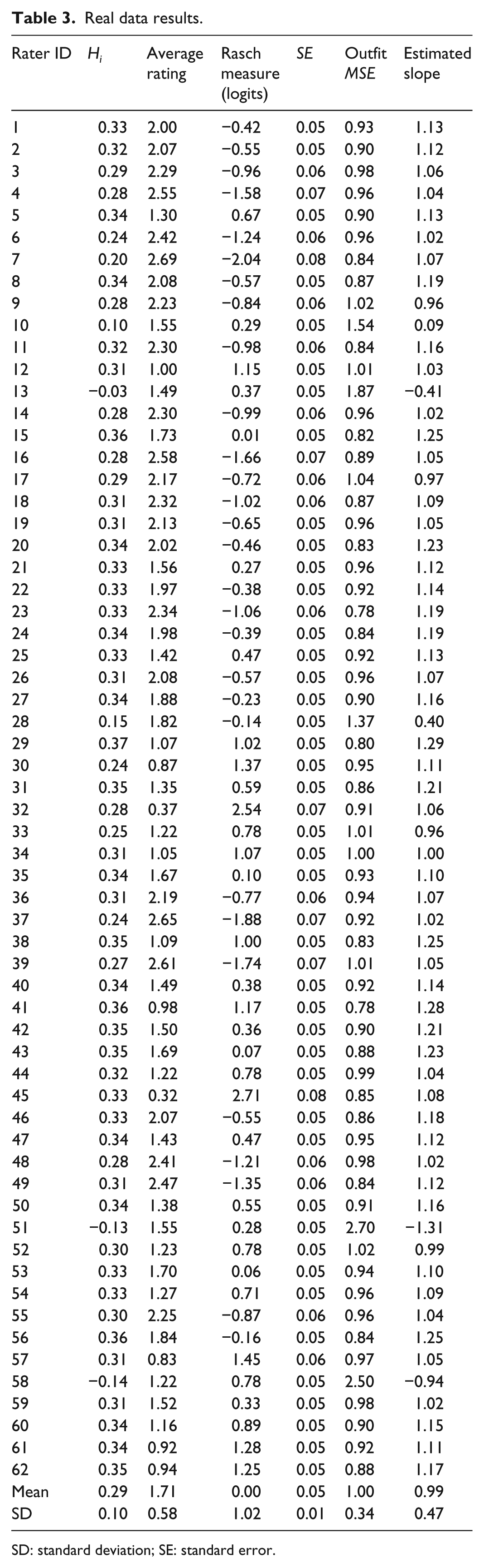
SD: standard deviation; SE: standard error.

For each of the 62 raters, Table 3 also includes values of the ac-MSA rater scalability coefficients (H_i), along with the two parametric rater fit statistics (Outfit MSE and estimated slope). Raters’ H_i coefficients ranged from H_i = −0.19 for Rater 5, who had the lowest scalability to H_i = 0.37 for Rater 46, who had the highest scalability. Further inspection of the values of H_i among these raters reveals that four raters had negative scalability coefficients (Raters 5, 21, 32, and 50). These values suggest that these raters exhibited more Guttman errors than would be expected based on chance alone. Among these raters, the average Outfit MSE statistic was 2.30 (SD = 0.33); this value is notably higher than 1.00, which is the value of Outfit MSE that several researchers have established as expected when there is acceptable fit to the RS model (Smith, 2004; Wu and Adams, 2013). Furthermore, the Outfit MSE statistics for each of these four raters are well above the critical values that several researchers have established for identifying raters who exhibit substantial model-data misfit (Bond and Fox, 2015; Engelhard and Wind, 2018). Likewise, it is interesting to note that the estimated slope parameters for each of these raters is negative (M = −0.86, SD = 0.41)—indicating substantial deviations from the RS model-expected value of 1.00. In contrast, the average Outfit MSE statistics and estimated slope parameters for the remaining 58 raters who have positive ac-MSA scalability coefficients are within the expected range when data fit the RS model (Outfit MSE: M = 0.92, SD = 0.07; α: M = 1.11, SD = 0.09).

Together, these results suggest that ac-MSA scalability coefficients for raters are sensitive to deviations from model-data fit based on the RS model—thus reflecting Guttman errors. These findings are further corroborated by results from the correlation analysis between H_i coefficients and the parametric fit statistics. Specifically, the correlation between Outfit MSE and H_i in the writing assessment data was strong and negative: r = −0.94 (t(60) = −21.35, p < 0.001). Figure 4 illustrates the bivariate relationship between Outfit MSE and H_i, where it can be seen that low values of H_i, which indicate the presence of many Guttman errors, correspond to high values of Outfit MSE, which indicate large and frequent residuals between observed ratings and RS model-expected ratings. I also examined the correlation between these two statistics without the four raters who had negative scalability coefficients, as these raters appeared to be outliers. Without these raters, the correlation was weaker (r = −0.40), but remained statistically significant (t(56) = −3.27, p < 0.001). Likewise, there was a strong and positive relationship between raters’ estimated slopes and values of H_i: r = 0.95 (t(60) = 22.54, p < 0.001); without the extreme misfitting raters, the correlation was r = 0.81 (t(53) = 9.94, p < 0.001). Figure 4 illustrates this relationship, where it can be seen that low values of H_i, which indicate the presence of many Guttman errors, correspond to low values of the estimated slope parameter, which indicate deviations from the Rasch model-expected value of 1.00.

Figure 4.

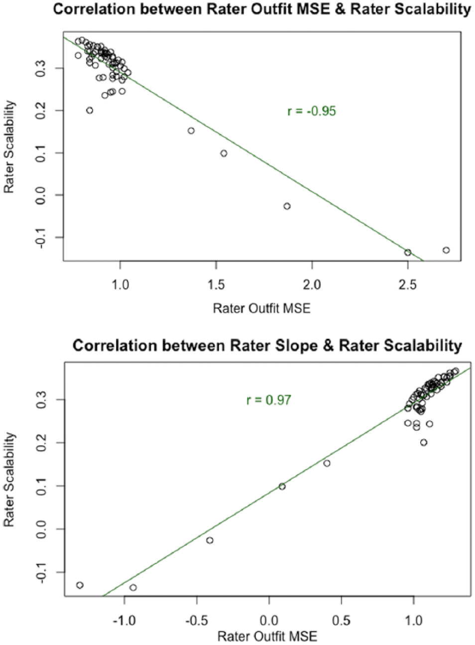
Correlations between rater scalability coefficients and parametric rater fit statistics.

To explore rater fit further using graphical displays, I examined nonparametric RRFs for each of the raters included in the writing assessment data. Considering the values of rater scalability coefficients and parametric fit statistics, I focused specifically on differences in RRFs between the raters who had negative H_i coefficients and raters who had positive H_i coefficients. Figures 5 and 6 illustrate the results from this analysis. Specifically, Figure 5 includes RRFs for the four raters who had negative ac-MSA scalability coefficients, and Figure 6 includes RRFs for four randomly selected raters who had non-negative ac-MSA scalability coefficients. Inspection of these two figures reveals that the RRFs for the four raters who had negative H_i coefficients (Figure 5) were either negatively sloped (e.g. Rater 5), or generally flat, with negative slopes over some regions of the x-axis. In contrast, the RRFs for the four raters in Figure 6 were non-decreasing over increasing levels of examinee achievement.

Figure 5.

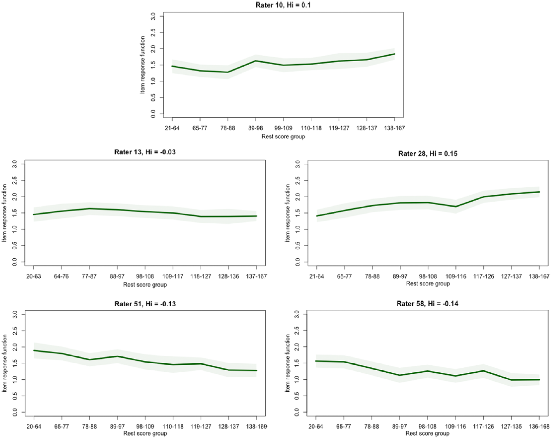
Rater response functions: raters with negative ac-MSA scalability coefficients (real data).

Figure 6.

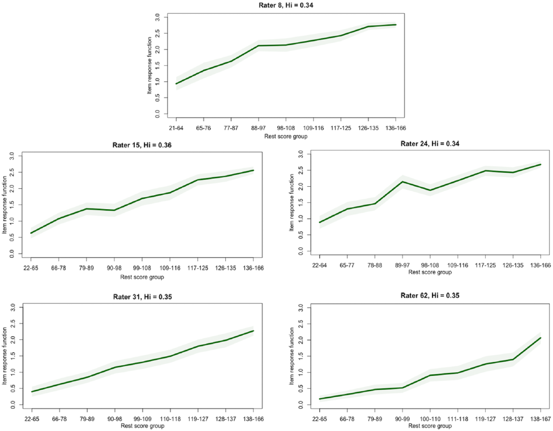
Rater response functions: raters with non-negative ac-MSA scalability coefficients (real data).

Quasi-simulated data results

Figure 7 presents boxplots that show the distribution of rater scalability coefficients, rater outfit MSE statistics, and rater estimated slope parameters in each of the four quasi-simulated datasets, along with the distribution in the original real dataset. Overall, the results suggest that the quasi-simulated datasets with smaller sample sizes reflect the general range of rater fit statistics as the original dataset. However, the boxplots indicate some variability in the values of each fit statistic as the sample sizes decreased.

Figure 7.

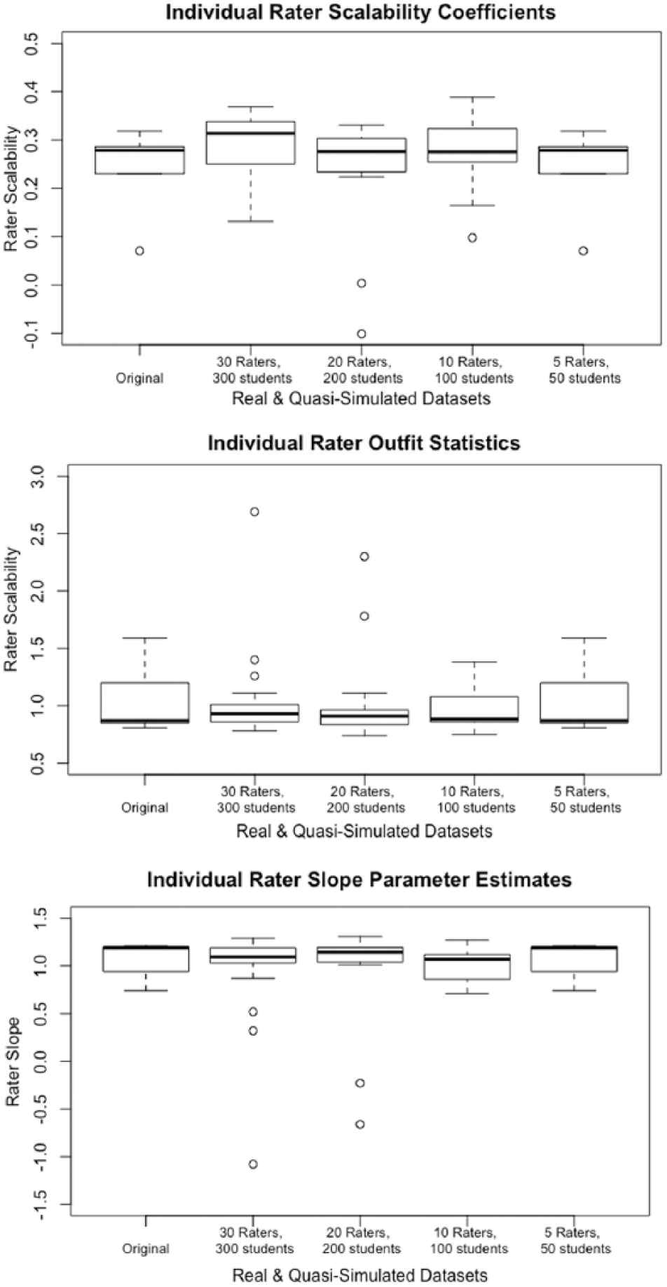
Distribution of rater fit statistics in the original and quasi-simulated datasets.

The correlations between rater scalability coefficients and each of the two parametric rater fit statistics showed similar patterns as the original real dataset. Across each of the four quasi-simulated datasets, there was a strong negative correlation between H_i and Outfit MSE (−0.72 ⩽ r ⩽ 0.94), and a strong positive correlation between H_i and the estimated rater slope parameter (0.55 ⩽ 0.96). I observed the weakest correlation between H_i and Outfit MSE (r = −0.72) in the quasi-simulated dataset in which I included 10 raters and 100 examinees, and the strongest correlation when I included 30 raters and 300 examinees (r = −0.94). The correlation between H_i and the estimated rater slope parameter was weakest in the smallest quasi-simulated dataset (5 raters and 50 examinees; r = 0.55) and strongest in the second-to-largest quasi-simulated dataset (20 raters and 200 examinees; r = 0.97). Finally, I examined nonparametric RRFs in each of the quasi-simulated datasets. These graphical displays reflected similar characteristics as the original dataset (see Figures 5 and 6).

Together, these results indicate that the relationship between H_i and the parametric rater fit statistics was generally stronger with larger sample sizes. However, the lack of a systematic pattern between the magnitude of the correlations and sample size indicates that these rater fit statistics were not completely dependent on the number of raters or examinees. Rather, the fit statistics reflect random variations in the raters and examinees who made up each of the quasi-simulated datasets.

Simulation study results

As a first step in my analysis of the simulated data, I evaluated the accuracy with which my simulation procedure produced ratings with the intended characteristics. Specifically, after I analyzed the simulated datasets using the RS model, I examined the distributions of estimated examinee achievement, rater severity, rater Outfit MSE statistics, and rater slope. Examinees and raters had average achievement and severity locations around 0.0 logits, respectively, with a standard deviation around 1.0. Furthermore, for the raters who I modeled to exhibit fit to the RS model, the average Outfit MSE statistic ranged from 0.92 ⩽ Mean Outfit MSE ⩽ 0.99. These values are slightly lower than the value researchers generally accept as evidence of acceptable model-data fit (around 1.00; Smith, 2004; Wu and Adams, 2013); however, this result is somewhat expected, because I modeled other raters in each dataset to exhibit misfit. For these raters, the average estimated slope ranged from 1.01 ⩽ α ⩽ 1.12, which is around the expected value of 1.00 when data fit the Rasch model. For the raters who I modeled to exhibit moderate misfit to the RS model, the average Outfit MSE statistic ranged from 1.25 ⩽ Mean Outfit MSE ⩽ 1.66, and the average estimated slope ranged from 0.03 ⩽ α ⩽ 0.54. For the raters who I modeled to exhibit extreme misfit to the RS model, the average Outfit MSE statistic ranged from 1.40 ⩽ Mean Outfit MSE ⩽ 2.50, and the average estimated slope ranged from −0.94 ⩽ α ⩽ 0.10. Together, these characteristics suggest that the simulation procedure generated ratings with the intended characteristics.

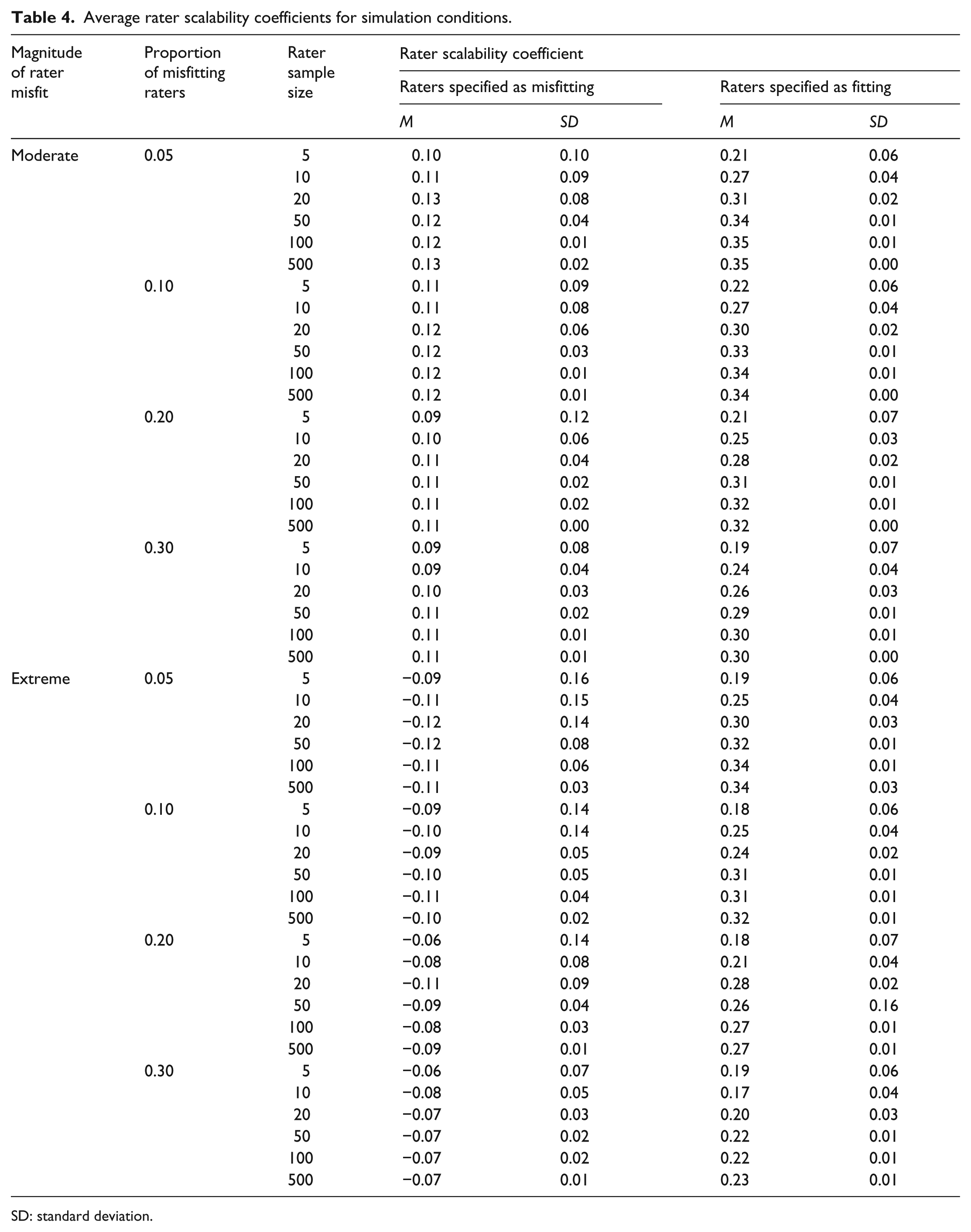
Table 4 presents the mean and standard deviation (SD) of the ac-MSA rater scalability coefficients (H_i) for each of the simulation conditions. In each condition, the average value of H_i was notably lower among the raters who I modeled to exhibit misfit to the RS model (−0.12 ⩽ H_i ⩽ 0.13) compared to the raters who I did not model to exhibit misfit (0.18 ⩽ H_i ⩽ 0.34). In the conditions in which I modeled extreme rater misfit, all of the average scalability coefficients for the misfitting raters were negative—indicating that these raters exhibited more Guttman errors than expected based on chance alone. Similarly, in the conditions in which I modeled moderate misfit, the average rater scalability coefficients for raters who I modeled to exhibit misfit were quite low (0.09 ⩽ H_i ⩽ 0.13). In every condition, the average scalability coefficients for the raters who I did not model to exhibit misfit were positive and at least two times higher than the average scalability coefficients for the raters who I modeled to exhibit misfit.

Table 4.

Average rater scalability coefficients for simulation conditions.

Magnitude of rater misfit	Proportion of misfitting raters	Rater sample size	Rater scalability coefficient
			Raters specified as misfitting		Raters specified as fitting
			M	SD	M	SD
Moderate	0.05	5	0.10	0.10	0.21	0.06
		10	0.11	0.09	0.27	0.04
		20	0.13	0.08	0.31	0.02
		50	0.12	0.04	0.34	0.01
		100	0.12	0.01	0.35	0.01
		500	0.13	0.02	0.35	0.00
	0.10	5	0.11	0.09	0.22	0.06
		10	0.11	0.08	0.27	0.04
		20	0.12	0.06	0.30	0.02
		50	0.12	0.03	0.33	0.01
		100	0.12	0.01	0.34	0.01
		500	0.12	0.01	0.34	0.00
	0.20	5	0.09	0.12	0.21	0.07
		10	0.10	0.06	0.25	0.03
		20	0.11	0.04	0.28	0.02
		50	0.11	0.02	0.31	0.01
		100	0.11	0.02	0.32	0.01
		500	0.11	0.00	0.32	0.00
	0.30	5	0.09	0.08	0.19	0.07
		10	0.09	0.04	0.24	0.04
		20	0.10	0.03	0.26	0.03
		50	0.11	0.02	0.29	0.01
		100	0.11	0.01	0.30	0.01
		500	0.11	0.01	0.30	0.00
Extreme	0.05	5	−0.09	0.16	0.19	0.06
		10	−0.11	0.15	0.25	0.04
		20	−0.12	0.14	0.30	0.03
		50	−0.12	0.08	0.32	0.01
		100	−0.11	0.06	0.34	0.01
		500	−0.11	0.03	0.34	0.03
	0.10	5	−0.09	0.14	0.18	0.06
		10	−0.10	0.14	0.25	0.04
		20	−0.09	0.05	0.24	0.02
		50	−0.10	0.05	0.31	0.01
		100	−0.11	0.04	0.31	0.01
		500	−0.10	0.02	0.32	0.01
	0.20	5	−0.06	0.14	0.18	0.07
		10	−0.08	0.08	0.21	0.04
		20	−0.11	0.09	0.28	0.02
		50	−0.09	0.04	0.26	0.16
		100	−0.08	0.03	0.27	0.01
		500	−0.09	0.01	0.27	0.01
	0.30	5	−0.06	0.07	0.19	0.06
		10	−0.08	0.05	0.17	0.04
		20	−0.07	0.03	0.20	0.03
		50	−0.07	0.02	0.22	0.01
		100	−0.07	0.02	0.22	0.01
		500	−0.07	0.01	0.23	0.01

SD: standard deviation.

Several other characteristics were interesting to note with regard to the variables that I manipulated in the simulation study. First, as the proportion of misfitting raters increased, the magnitude of the difference in the average H_i between the raters who I modeled to exhibit misfit and the raters who I did not model to exhibit misfit generally decreased. For example, in the conditions where I modeled 5% of the rater sample size to exhibit misfit, the absolute value of the difference (|Δ|) in the average H_i between the two groups of raters ranged from 0.11 ⩽ |Δ| ⩽ 0.45. In contrast, in the conditions where I modeled 30% of the rater sample size to exhibit misfit, the absolute value of the difference in the average H_i between the two groups of raters ranged from 0.10 ⩽ |Δ| ⩽ 0.30. Second, it is interesting to note that there were only small differences in the average values of H_i across the rater sample sizes, with slightly higher values of H_i (suggesting better rater fit, on average), when more raters were included. This result indicates that the total number of raters does not appear to have a meaningful impact on the influence of Guttman errors on values of H_i.

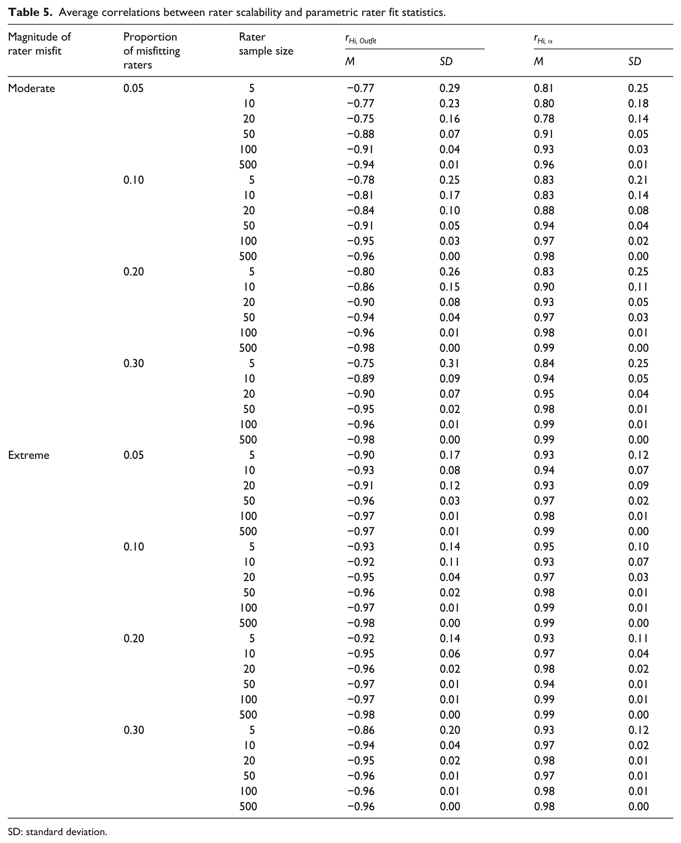
Table 5 includes results from the correlation analyses of the simulated data. The patterns of correlations between rater scalability coefficients and the parametric rater fit statistics were similar to the correlations in the real data. Across conditions, the average correlation between rater scalability coefficients and Outfit MSE was strong and negative (−0.75 ⩽ r ⩽ −0.98)—suggesting that lower values of rater scalability coefficients, which suggest more frequent Guttman errors, were associated with higher values of Outfit MSE, which suggest more frequent departures from Rasch model expectations (i.e. more extreme misfit). The correlations were somewhat stronger in the conditions in which I modeled extreme rater misfit (−0.90 ⩽ r ⩽ −0.98) compared to the conditions in which I modeled moderate rater misfit (−0.75 ⩽ r ⩽ −0.98), particularly among the smaller sample size conditions. Also reflecting the real data results, the average correlation between rater scalability coefficients and estimated rater slopes was strong and positive in all of the simulation conditions (0.78 ⩽ r ⩽ 0.99). Similar to the correlation between scalability and Outfit, this relationship was stronger in the conditions in which I modeled extreme rater misfit (0.93 ⩽ r ⩽ 0.99) compared to the conditions in which I modeled moderate rater misfit (0.78 ⩽ r ⩽ 0.99), particularly among the conditions with smaller rater sample sizes. This result indicates that low values of rater slope, which indicate large and frequent residuals between observed ratings and RS model-expected ratings, were associated with low values of rater scalability, which indicate frequent Guttman errors.

Table 5.

Average correlations between rater scalability and parametric rater fit statistics.

Magnitude of rater misfit	Proportion of misfitting raters	Rater sample size	r_{Hi, Outfit}		r_{Hi, α}
Magnitude of rater misfit	Proportion of misfitting raters	Rater sample size	M	SD	M	SD
Moderate	0.05	5	−0.77	0.29	0.81	0.25
		10	−0.77	0.23	0.80	0.18
		20	−0.75	0.16	0.78	0.14
		50	−0.88	0.07	0.91	0.05
		100	−0.91	0.04	0.93	0.03
		500	−0.94	0.01	0.96	0.01
	0.10	5	−0.78	0.25	0.83	0.21
		10	−0.81	0.17	0.83	0.14
		20	−0.84	0.10	0.88	0.08
		50	−0.91	0.05	0.94	0.04
		100	−0.95	0.03	0.97	0.02
		500	−0.96	0.00	0.98	0.00
	0.20	5	−0.80	0.26	0.83	0.25
		10	−0.86	0.15	0.90	0.11
		20	−0.90	0.08	0.93	0.05
		50	−0.94	0.04	0.97	0.03
		100	−0.96	0.01	0.98	0.01
		500	−0.98	0.00	0.99	0.00
	0.30	5	−0.75	0.31	0.84	0.25
		10	−0.89	0.09	0.94	0.05
		20	−0.90	0.07	0.95	0.04
		50	−0.95	0.02	0.98	0.01
		100	−0.96	0.01	0.99	0.01
		500	−0.98	0.00	0.99	0.00
Extreme	0.05	5	−0.90	0.17	0.93	0.12
		10	−0.93	0.08	0.94	0.07
		20	−0.91	0.12	0.93	0.09
		50	−0.96	0.03	0.97	0.02
		100	−0.97	0.01	0.98	0.01
		500	−0.97	0.01	0.99	0.00
	0.10	5	−0.93	0.14	0.95	0.10
		10	−0.92	0.11	0.93	0.07
		20	−0.95	0.04	0.97	0.03
		50	−0.96	0.02	0.98	0.01
		100	−0.97	0.01	0.99	0.01
		500	−0.98	0.00	0.99	0.00
	0.20	5	−0.92	0.14	0.93	0.11
		10	−0.95	0.06	0.97	0.04
		20	−0.96	0.02	0.98	0.02
		50	−0.97	0.01	0.94	0.01
		100	−0.97	0.01	0.99	0.01
		500	−0.98	0.00	0.99	0.00
	0.30	5	−0.86	0.20	0.93	0.12
		10	−0.94	0.04	0.97	0.02
		20	−0.95	0.02	0.98	0.01
		50	−0.96	0.01	0.97	0.01
		100	−0.96	0.01	0.98	0.01
		500	−0.96	0.00	0.98	0.00

SD: standard deviation.

As I did with the real and quasi-simulated data, I also examined rater fit in the simulated datasets using nonparametric RRFs. Specifically, I randomly selected 30 replications from each of the simulation conditions and examined RRFs for raters who I modeled to exhibit misfit and raters who I did not model to exhibit misfit. The general characteristics of the RRFs for these raters matched those that I observed in the real data analysis. That is, raters who I modeled to exhibit misfit displayed either flat or negatively sloped RRFs, and raters who I modeled to exhibit acceptable fit displayed generally positive RRFs.

Discussion

The purpose of this study was to present and illustrate an approach to evaluating rater fit using Guttman errors. Because Guttman errors are related to invariant measurement, they provide a useful nonparametric method for evaluating rating quality that is appropriate for numerous situations in which raters use ordinal rating scales to evaluate test-taker achievement. In contrast to atheoretical nonparametric approaches to evaluating rating quality, such as kappa or rater agreement statistics, the approach illustrated in this study provides researchers and practitioners with detailed information about individual raters that is grounded within the framework of invariant measurement. Using data from a rater-mediated writing assessment, I demonstrated how researchers and practitioners can use adjacent-categories scalability coefficients and nonparametric RRFs to identify raters who exhibit problematic rating patterns.

The results from this study have several implications for research and practice related to rater-mediated assessments. Previously, several researchers have explored the utility of Guttman errors to identify test-takers whose total scores may not be reasonable summaries of their locations on a construct (Meijer, 1994), as well as items that do not function consistently across persons (Molenaar, 1991). The results from this study suggest that researchers and practitioners can use summaries of Guttman errors as a tool for exploring rater fit from the perspective of invariant measurement. The nonparametric approach to exploring rating quality illustrated in this study is useful because it allows researchers and practitioners to consider rating quality in terms of important properties, such as invariance, without imposing potentially inappropriate transformations on ordinal ratings. Furthermore, researchers can use this nonparametric approach to explore the measurement characteristics of a rater-mediated assessment prior to the application of a parametric model.

When interpreting the results from this study, several limitations are important to note. First, because the characteristics of the writing assessment data and the data that I simulated do not reflect every rater-mediated writing assessment, researchers and practitioners should consider the alignment between the characteristics of the data included in this analysis and other assessment contexts before generalizing the results beyond the scope of this study. Second, it is important to note that researchers have proposed other methods for summarizing Guttman errors, including counts of Guttman errors (Meijer, 1994), and other forms of scalability coefficients (Kuijpers et al., 2013; Molenaar, 1991). In future studies, researchers should consider the degree to which other summaries of Guttman errors, as well as other rater fit indices based on nonparametric IRT share the characteristics observed in this study.

Footnotes

Acknowledgements

A previous version of this paper was presented at the meeting of the International Objective Measurement Workshop in New York, New York, April 2018.

Declaration of conflicting interests

The author(s) declared no potential conflicts of interest with respect to the research, authorship, and/or publication of this article.

Funding

The author(s) received no financial support for the research, authorship, and/or publication of this article.

Notes

ORCID iD

Stefanie A Wind

Author biography

Stefanie A Wind is an Assistant Professor of Educational Measurement at the University of Alabama. Her primary research interests include the exploration of methodological issues in the field of educational measurement, with emphases on methods related to rater-mediated assessments, rating scales, Rasch models and item response theory models, and nonparametric item response theory, as well as applications of these methods to substantive areas related to education.

References

Andrich

(1978) A rating formulation for ordered response categories. Psychometrika 43(4): 561–573.

Bond

Fox

(2015) Applying the Rasch Model: Fundamental Measurement in the Human Sciences (3rd edn). New York: Routledge.

Brown

Glasswell

Harland

(2004) Accuracy in the scoring of writing: Studies of reliability and validity using a New Zealand writing assessment system. Assessing Writing 9: 105–121.

Cohen

(1968) Weighted kappa: Nominal scale agreement provision for scaled disagreement or partial credit. Psychological Bulletin 70(4): 213–220.

Commonwealth of Virginia, Department of Education (2012) Virginia Standards of Learning Assessments Test Blueprint: End of Course Writing. Richmond, VA. Available at: http://www.doe.virginia.gov/testing/sol/blueprints/english_blueprints/2010/2010_blueprint_eoc_writing.pdf

Duckor

Castellano

Téllez

et al . (2014) Examining the internal structure evidence for the performance assessment for California teachers: A validation study of the elementary literacy teaching event for Tier I teacher licensure. Journal of Teacher Education 65(5): 402–420.

Eckes

(2015) Introduction to Many-Facet Rasch Measurement: Analyzing and Evaluating Rater-Mediated Assessments (2nd edn). Frankfurt am Main: Peter Lang.

Engelhard

(1994) Examining rater errors in the assessment of written composition with a many-faceted Rasch model. Journal of Educational Measurement 31(2): 93–112.

Engelhard

(1997) Constructing rater and task banks for performance assessments. Journal of Outcome Measurement 1(1): 19–33.

10.

Engelhard

Wind

(2018) Invariant Measurement with Raters and Rating Scales: Rasch Models for Rater-Mediated Assessments. New York: Taylor & Francis.

11.

Freedland

Lemos

Doyle

et al . (2016) The techniques for overcoming depression questionnaire: Mokken scale analysis, reliability, and concurrent validity. Journal of Psychosomatic Research 85: 65.

12.

Georgia Department of Education (2015) Writing assessments. Available at: http://www.gadoe.org/Curriculum-Instruction-and-Assessment/Assessment/Pages/Writing-Assessments.aspx

13.

Gillespie

Tenvergert

Kingma

(1988) Using Mokken methods to develop robust cross-national scales: American and West German attitudes toward abortion. Social Indicators Research 20(2): 181–203.

14.

Junker

Sijtsma

(2001) Cognitive assessment models with few assumptions, and connections with nonparametric item response theory. Applied Psychological Measurement 25(3): 258–272.

15.

Kaliski

Wind

Engelhard

et al . (2013) Using the many-faceted Rasch model to evaluate standard setting judgments: An illustration with the advanced placement environmental science exam. Educational and Psychological Measurement 73(3): 386–411.

16.

Kuijpers

Van der Ark

Croon

(2013) Standard errors and confidence intervals for scalability coefficients in Mokken scale analysis using marginal models. Sociological Methodology 43(1): 42–69.

17.

Linacre

(2015) Facets Rasch Measurement (Version 3.71.4). Chicago, IL: Winsteps.com.

18.

Marais

Andrich

(2011) Diagnosing a common rater halo effect using the polytomous Rasch model. Journal of Applied Measurement 12(3): 194–211.

19.

Meijer

(1994) The number of Guttman errors as a simple and powerful person-fit statistic. Applied Psychological Measurement 18(4): 311–314.

20.

Meijer

Baneke

(2004) Analyzing psychopathology items: A case for nonparametric item response theory modeling. Psychological Methods 9(3): 354–368.

21.

Mokken

(1971) A Theory and Procedure of Scale Analysis. The Hague: Mouton/Berlin: De Gruyter.

22.

Molenaar

(1991) A weighted Loevinger H-coefficient extending Mokken scaling to multicategory items. Kwantitative Methoden 37(12): 97–117.

23.

Molenaar

(1982) Mokken scaling revisited. Kwantitative Methoden 3(8): 145–164.

24.

Molenaar

(1997) Nonparametric models for polytomous responses. In Handbook of modern item response theory. New York: Springer, pp. 369–380.

25.

Molenaar

Sijtsma

(2000) MPS5 for Windows: A Program for Mokken Scale Analysis for Polytomous Items (Version 5.0). Groningen, The Netherlands: ProGAMMA.

26.

Molenaar

(2001) Thirty years of nonparametric item response theory. Applied Psychological Measurement 25(3): 295–299.

27.

Muncer

Speak

(2016) Mokken scale analysis and confirmatory factor analysis of the health of the nation outcome scales. Personality and Individual Differences 94: 272–276.

28.

Muraki

(1997) A generalized partial credit model. In: Van der Linden

Hambleton

(eds) Handbook of Modern Item Response Theory. New York: Springer, pp. 153–164.

29.

Myford

Wolfe

(2004) Detecting and measuring rater effects using many-facet Rasch measurement: Part II. Journal of Applied Measurement 5(2): 189–227.

30.

NAEP Writing-Achievement Level Details (n.d.) The NAEP Writing Achievement Levels. Washington, DC: National Assessment of Educational Progress. Available at: https://nces.ed.gov/nationsreportcard/writing/achieve.aspx

31.

Paas

(1999) Refining RFM-variables through Mokken scale analysis for the purpose of optimal prospect selection: Application to ownership patterns of financial products. Journal of Market-Focused Management 3(3–4): 275–294.

32.

R Core Team (2018) R: A Language and Environment for Statistical Computing. Vienna, Austria: R Foundation for Statistical Computing. Available at: https://www.R-project.org/

33.

Rasch

(1960) Probabilistic models for some intelligence and achievement tests (Expanded edition, 1980). Chicago, IL: University of Chicago Press.

34.

Raczynski

Cohen

Engelhard

et al . (2015) Comparing the effectiveness of self-paced and collaborative frame-of-reference training on rater accuracy in a large-scale writing assessment. Journal of Educational Measurement 52: 301–318.

35.

Reise

Waller

(2003) How many IRT parameters does it take to model psychopathology items? Psychological Methods 8(2): 164–184.

36.

Santor

Ramsay

(1998) Progress in the technology of measurement: Applications of item response models. Psychological Assessment 10(4): 345–359.

37.

Schumacker

(2015) Detecting measurement disturbance effects: The graphical display of item characteristics. Journal of Applied Measurement 16(1): 76–81.

38.

Sijtsma

Molenaar

(2002) Introduction to Nonparame-tric Item Response Theory, vol. 5. Thousand Oaks, CA: SAGE.

39.

Smith

(2004) Fit analysis in latent trait models. In: Smith

Smith

(eds) Introduction to Rasch Measurement. Maple Grove, MN: JAM Press, pp. 73–92.

40.

Van der Veer

Yakushko

Ommundsen

et al . (2011) Cross-national measure of fear-based xenophobia: Development of a cumulative scale. Psychological Reports 109(1): 27–42.

41.

Wind

(2016) Adjacent-categories Mokken models for rater-mediated assessments. Educational and Psychological Measurement 77: 330–350.

42.

Wind

Peterson

(2017) A systematic review of methods for evaluating rating quality in language assessment. Language Testing 35(2): 161–192. doi:10.1177/0265532216686999

43.

Wind

Schumacker

(2017) Detecting measurement disturbances in rater-mediated assessments. Educational Measurement: Issues and Practice 36: 44–51.

44.

Wind

Engelhard

Wesolowski

(2016) Exploring the effects of rater linking designs and rater fit on achievement estimates within the context of music performance assessments. Educational Assessment 21(4): 278–299.

45.

Wolfe

(1998) A Two-Parameter Logistic Rater Model (2PLRM): Detecting Rater Harshness and Centrality. San Diego, CA: American Educational Research Association.

46.

Wolfe

McVay

(2012) Application of latent trait models to identifying substantively interesting raters. Educational Measurement: Issues and Practice 31(3): 31–37.

47.

Wolfe

Song

(2015) Comparison of models and indices for detecting rater centrality. Journal of Applied Measurement 16(3): 228–241.

48.

Wolfe

Jiao

Song

(2014) A family of rater accuracy models. Journal of Applied Measurement 16(2): 153–160.

49.

Wolfe

Matthews

Vickers

(2010) The effectiveness and efficiency of distributed online, regional online, and regional face-to-face training for writing assessment raters. Journal of Technology, Learning, and Assessment 10: 1–21.

50.

Adams

(2013) Properties of Rasch residual fit statistics. Journal of Applied Measurement 14(4): 339–355.

Using Guttman errors to explore rater fit in rater-mediated performance assessments

Abstract

Keywords

Nonparametric IRT methods for evaluating rater fit

Purpose

Scalability coefficients

Polytomous scalability coefficients

Methods

Real data

Quasi-simulated real data

Simulated data

Variables held constant

Manipulated variables

Data analysis

Results

Real data results

Quasi-simulated data results

Simulation study results

Discussion

Footnotes

Acknowledgements

Declaration of conflicting interests

Funding

Notes

ORCID iD

Author biography

References