Resolving the test–retest agreement or reliability dilemma

Abstract

Agreement refers to the degree to which an individual i’s test scores match in test–retest settings. Agreement has been thought to be unapproachable with correlational reliability indices. Stable unstable reliability theory extends Spearman’s reliability model and specifies the probability that i’s test–retest true scores match. Thus, agreement and reliability are simultaneously addressed. Two examples, one using longitudinal data, illustrate the procedure.

Introduction

In test–retest settings (Berchtold, 2016), reliability is “… the capacity of a test to replicate the same ordering between respondents when measured twice.” More important is agreement. It requires “… the same exact result that each respondent obtains on the two testing occasions” (Berchtold, 2016: 1). That is, test–retest observed scores match for each individual $i$ . That agreement is typically unspecified is Berchtold’s principal concern, particularly as agreement relates to longitudinal studies. His example concerns a sample of 678 French-speaking Swiss adolescents responding to the Internet Addiction Test (IAT) test and 5 months later completing a retest. The retest showed a significant mean decrease of 2.77 from the first test. The vexing issue for Berchtold is “… given the small amount of change between the two testing occasions … and the fact that the IAT was evaluated for reliability, but not for agreement, can we really conclude that the IAT is lower” on the second administration than on the first? For Berchtold (2016), the “question is still open (p. 2).”

This article has two goals. The first goal is to resolve the agreement or reliability dilemma by showing that by empirically testing an assumption in Spearman’s random-effects model of correlation (Spearman, 1910; Yule, 1932), the agreement issue can be addressed at the level of each individual $i$ . The second goal is to illustrate the theory’s implementation in two examples; the second example explores Berchtold’s IAT longitudinal data.

In 1904, Charles Spearman introduced the notion of reliability in the literature. His name remains associated with the term’s use, at least in the educational and psychological literature. However, no authoritative source has defined reliability as replicating “the same ordering” on both testing occasions (e.g. Gulliksen, 1950; Lord, 1986; Lord and Novick, 1968; Yule, 1932).

However, Berchtold’s definition of agreement is similar to Spearman’s reliability assumption, namely that each i’s test–retest true scores match. Another way to represent agreement for Berchtold (2016), Bland and Altman (2010 [1986]), and Kottner et al. (2011), among others, is to state that equivalently, pairs of observed scores must lie on a scatter plot’s identity line for agreement to be satisfied, while under Spearman’s reliability theory pairs of true scores (defined below) are assumed to lie on a scatter plot’s identity line. The conceptual difference between defining agreement as based on observed scores and a model-based approach which defines agreement as based on expected scores is crucial, as will be seen.

The extension of Spearman’s model is called stable unstable reliability theory or SURT. Through SURT, empirical tests of Spearman’s assumption are made, and the probability that i’s true scores match is provided. The main ideas of SURT are given below. Details appear elsewhere (Thomas et al., 2012).

SURT in brief

Key points

• If inference at the $i$ level is desired, modeling must start at the $i$ level.

• The response random variable is a latent structure.

• Matching of test–retest scores (i.e. agreement) is matching of expectations.

Consider modeling i’s IAT scores. Before each measurement is observed, i’s realized values are unknown: That is, they are random variables which are invisible, unobservable quantities. Denote two continuous random variables, $Y_{i|j}\mathrm{,}j=1,2,$ where $j$ denotes the first or second IAT test for $i$ . Only realizations of random variables (outcomes) are observable. After responses are rendered, the realized values are for $i$ , for example, $y_{i|1}=11$ and $y_{i|2}=9.$ Random variables are denoted by capitals, and realizations are denoted by lower case letters. The issue is to determine how i’s matching on two trials should be conceptualized. This defines agreement at the $i$ level.

Now consider how Berchtold (2016) and others define agreement: It is matching of each i’s realized values (he uses the term realized) and adds for emphasis “the same exact values” (p. 3). This implies matching occurs when $y_{i|1}=y_{i|2}$ . However, matching on realized values is conceptually fatal for two reasons. First, it ignores the fact that observed realized scores are contaminated with observational or measurement error. So matching on observed scores means matching on perturbed values of continuous variables; such a definition of agreement is conceptually indefensible. Second, matching on realized values is a non-starter if probabilistic structures are to play a role in the evaluation of such matches because to do so requires that continuous random variables take on point values. $Y_{i|1}=y_{i|1}$ and $Y_{i|2}=y_{i|2}$ with equality in realizations for agreement to be satisfied: $y_{i|1}=y_{i|2}$ . However, the probability of a continuous random variable taking on any point value is always zero because probability is defined as “area under a curve.” Consider random variable $Y$ with realizations $y$ and density (probability distribution) $f(y)$ . For i’s first IAT of 11, $P(Y=y=11)={\int }_{11}^{11}f(y)\mathrm{d}y$ which in calculus is zero. Consequently, both $P(Y_{i|1}=11)$ and $P(Y_{i|2}=9)$ are zero and so is their joint probability.

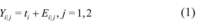
A conceptual path forward was proposed by Spearman (1910) and developed by Yule (1932). Define $Y_{i|j}$ as follows

$$Y_{i|j}=t_i+E_{i|j}\mathrm{,}j=1,2$$

(1)

This adds a conceptual layer, with $t_i$ being i’s true score, a fixed individual parameter, and $E_{i|j}$ is a mean zero error random variable. This is Spearman’s “true score error score” latent variable model at the individual $i$ level. Only values of $y_{i|j}$ are observed, while the right-hand side of equation (1) is latent and unobserved. Now each $i$ can have a unique expectation, and it is matching on expectations or true scores that is desired because $\mathrm{E}(Y_{i|j})=t_i$ unperturbed by error (E denotes expectation). Consequently, it is defined following SURT

• $i$ is stable iff $\mathrm{E}(Y_{i|1})=\mathrm{E}(Y_{i|2})$ ;

• $i$ is unstable iff $\mathrm{E}(Y_{i|1})\ne \mathrm{E}(Y_{i|2})$ .

It is stability that is required for agreement. Instability implies, of course, that i’s true scores are different for each $j$ (which is not represented in the current notation). Spearman’s model assumes that all $i$ are stable. SURT allows this assumption to be evaluated empirically. So, how can i’s stability be specified?

SURT estimation

Leave the bivariate correlational setting for the univariate difference score setting using $y_{i|1}-y_{i|2}$ to determine the probability $i$ is stable, denoted as $w_i$ . Then carry $w_i$ back to the correlational setting where $w_i$ and associated quantities can be informative in multiple ways.

If $i$ is stable, the expected value of the differences is zero: $\mathrm{E}(Y_{i|1}-Y_{i|2})=0$ . Should $i$ be unstable, $\mathrm{E}(Y_{i|1}-Y_{i|2})\ne 0$ . So stable $i$ differences will follow a distribution with mean zero, and unstable $i$ differences will follow a distribution with mean non-zero. Determining which distribution $i$ follows is nearly a standard finite mixture distribution problem (Everitt and Hand, 1981). Now assume the error random variables in equation (1), $E_{i|j}\mathrm{,}j=1,2$ , are independent and normal in distribution, then the distribution of the difference $Y_{i|1}-Y_{i|2}$ is normal. This puts the problem into a normal mixture setting where the probability $w_i$ that $i$ follows the normal distribution with mean zero is part of the standard algorithmic output. The procedure is easy to implement with the R call normalmixEM in the R package mixtools (Benaglia et al., 2009).

Example 1: peak expiratory flow rate measures

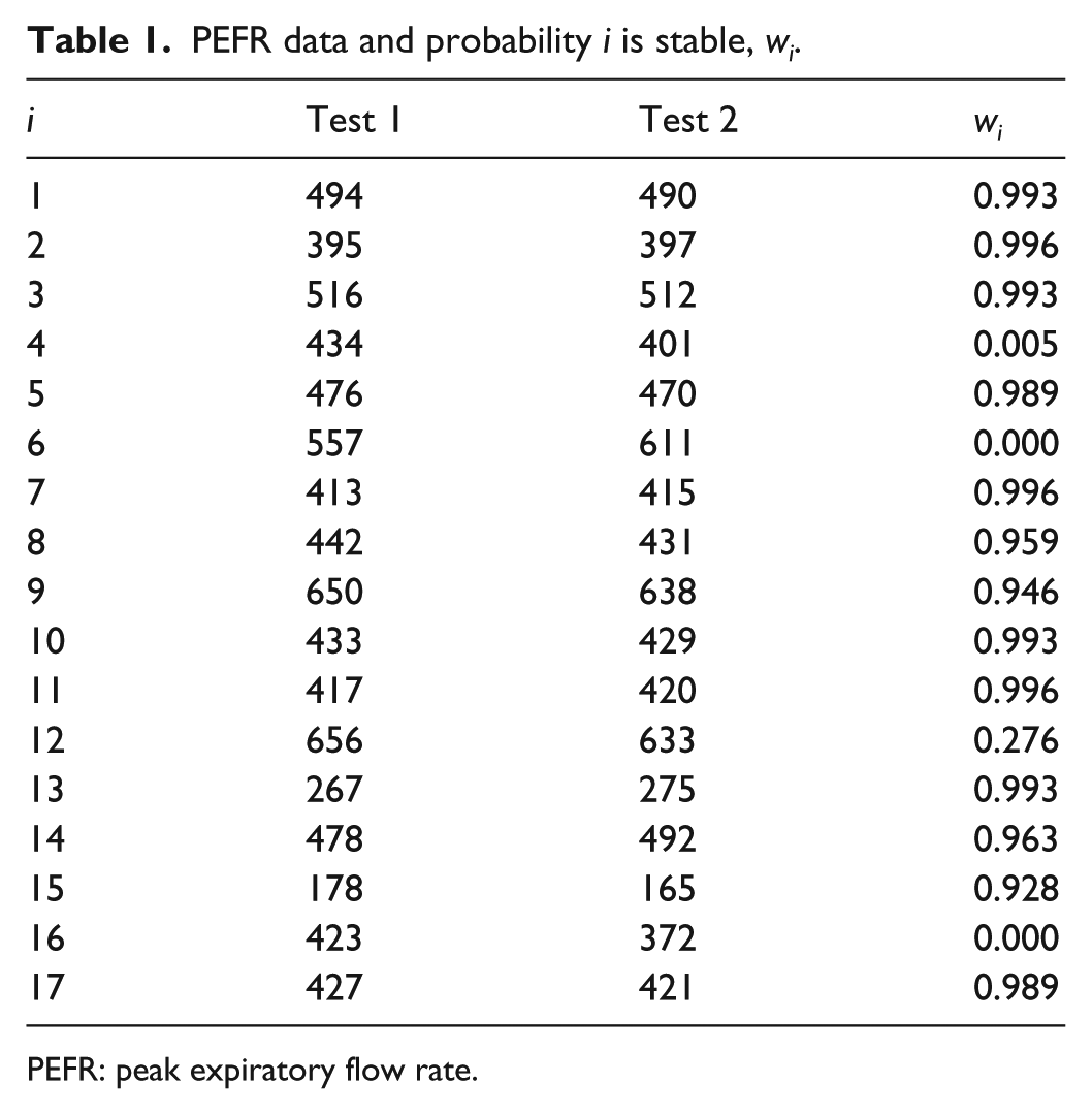
Bland and Altman (2010 [1986], cited in Berchtold, 2016 and republished in 2010) report test–retest data of 17 subjects measured for peak expiratory flow rate (PEFR; see Table 1). The analysis follows Example 1, 5.1 in Thomas et al. (2012). $w_i$ estimates are given in Table 1. (Only a very small portion of the output available is reported here.) Figure 1 is a bivariate data plot with circle size surrounding each data point proportional to i’s probability of being stable, $w_i$ ; the diagonal is the identity line.

Table 1.

PEFR data and probability i is stable, w_i.

i	Test 1	Test 2	wi
1	494	490	0.993
2	395	397	0.996
3	516	512	0.993
4	434	401	0.005
5	476	470	0.989
6	557	611	0.000
7	413	415	0.996
8	442	431	0.959
9	650	638	0.946
10	433	429	0.993
11	417	420	0.996
12	656	633	0.276
13	267	275	0.993
14	478	492	0.963
15	178	165	0.928
16	423	372	0.000
17	427	421	0.989

PEFR: peak expiratory flow rate.

Figure 1.

Test 2 plotted against Test 1 with identity line and circle size proportional to w_i.

Table 1 reveals that individuals 4, 6, and 16 are unstable. These individuals are easily identified in Figure 1 as points without surrounding circles and with stable $w_i$ probabilities of 0 or 0.005; $i=12$ is likely unstable; $w_{12}=0.276$ . The remaining 13 individuals are likely stable with $w_i\mathrm{s}$ ranging from 0.928 to 0.996.

Many quantities can be computed depending on one’s interest. For example, focus on those stable $i$ : $\mathrm{E}(Y_{i|1}-Y_{i|2})=0$ , $\mathrm{var}(Y_{i|1}-Y_{i|2})=\mathrm{var}(Y_{i|1}+Y_{i|2})={\mathrm{\sigma }}^2$ , and $\mathrm{var}((Y_{i|1}+Y_{i|2})/2)={\mathrm{\sigma }}^2/4$ . $\mathrm{E}((Y_{i|1}+Y_{i|2})/2)=t_i$ , with estimate $(y_{i|1}+y_{i|2})/2={\widehat{t}}_i$ . For each $i$ , stable ${\widehat{t}}_i$ has a normal distribution (forced by the mixtools procedure) with mean $t_i$ and standard deviation $\mathrm{\sigma }/2$ . The estimate of $\widehat{\mathrm{\sigma }}=8.54$ is from mixtools. Following Yule (1932: 211), consider $\widehat{\mathrm{\sigma }}/2=4.27$ as the “errors of observation” estimated standard deviation. Consider $i=1\mathrm{and}\$t1=492$ , and a 95% confidence interval for $t_1$ is about 484–500. Or comparing $i=1$ and $i=2$ , their estimated true scores are about 22 standard deviations apart.

Confidence intervals and tests can be constructed for almost all quantities of interest under SURT either from the standard theory or with the bootstrap (Efron and Tibshirani, 1993).

The main focus of SURT is to estimate reliability, with Spearman’s random-effects model correlation as a guide which is a population (over all $i$ ) estimate of true score variance over total score variance. The conventional estimate is usually the Pearson Test 1 and Test 2 correlation coefficient, $r$ . Under SURT, this estimate is altered by weighing the quantities in $r$ with $w_i$ ; the resulting $r$ is denoted as $r_w$ . In the PEFR example, $r_w=0.997$ , while $r=0.983$ for the Table 1 data. In this example, $r$ and $r_w$ are nearly the same. The difference in magnitude between $r$ and $r_w$ will be determined by where, in the configuration of points, the unstable individuals are located.

If one’s oracle could specify which $n^{\prime }i$ among a sample of $n$ are stable, because Spearman’s model assumes $i$ is stable, one would sensibly use just those $n^{\prime }i$ in computing $r$ . Consider $r_w$ as an estimate of this idealized world.

Example 2: Berchtold’s IAT data

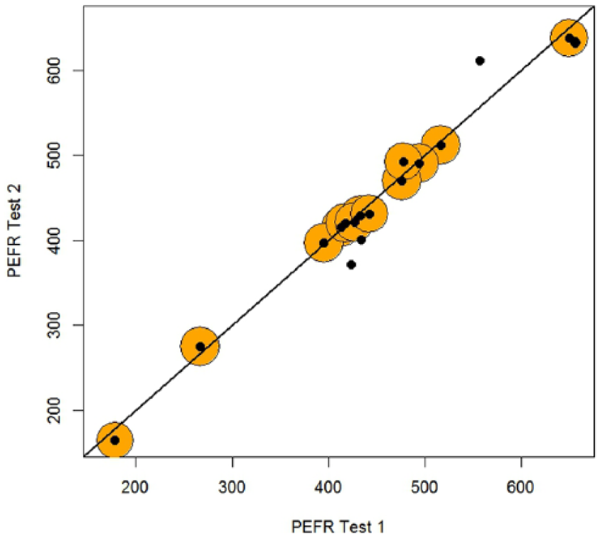
Usually when reliability is considered, the test–retest interval is such that individuals are assumed to remain stationary between tests. For some adolescents, after 5 months there can be large changes, and so it should not be surprising to see many unstable $i$ . Berchtold’s IAT data ¹ scatter plot displayed in Figure 2 can be interpreted just as in Figure 1 with points surrounded by circles in proportion to $w_i$ , the probability of i’s difference scores being from a mean zero stable normal distribution. Many points have no surrounding circle, signaling a zero probability of being stable. The proportion estimated as stable is 0.36, and so most individuals are unstable. The test–retest $r=0.71$ , while $r_w=\mathrm{0.94.}$ If $w_i=0,$ $i$ does not contribute to $r_w$ .

Figure 2.

Second IAT test plotted against first IAT test with circle size proportional to w_i; the line is the identity line.

The above is premised on the assumption that $\mathrm{E}(Y_{i|1}-Y_{i|2})=0$ for all $i$ stable. To address Berchtold’s concern as to whether, when controlling for stability, the retest mean is less than the first test mean, a notational and definitional change is required, so $i$ can have different true scores at each testing: $\mathrm{E}(Y_{i|j})=t_{i|j}\mathrm{,}j=1,2$ . Now redefine stability:

• $i$ is stable iff $\mathrm{E}(Y_{i|1}-\alpha )=\mathrm{E}(Y_{i|2})$ .

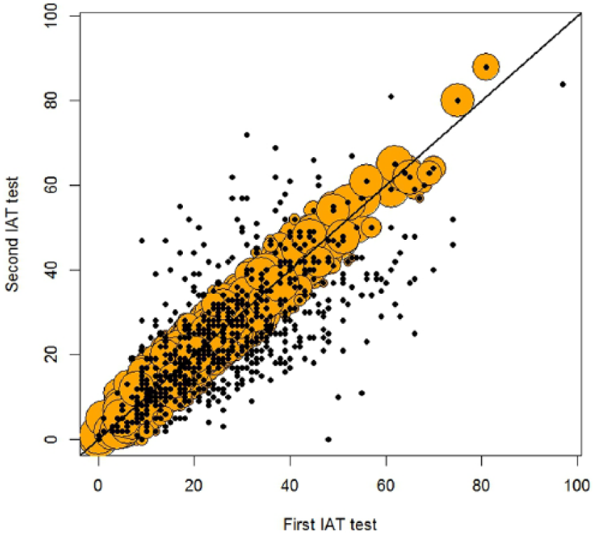
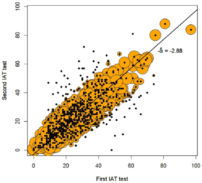
The shift parameter $\alpha =t_{i|1}-t_{i|2}$ . Stable $i$ difference scores follow a normal distribution with mean $\alpha$ , while unstable $i$ difference scores follow distributions with other means. Figure 3 shows the SURT solution with estimate $\widehat{\alpha }=2.88$ . The estimated proportion of $i$ that is stable is 0.62, while $r_w=0.87$ , the SURT reliability.

Figure 3.

Second IAT test plotted against first IAT test with circle size proportional to $w_i$ , with shift $-\widehat{\alpha }=-2.88$ line.

To determine which of the two solutions represented in Figures 2 and 3 is most appropriate, a penalized log likelihood criterion Bayesian Information Criterion (BIC; McLachlan and Peel, 2000) is used. The larger of the two BIC solutions is declared “the winner.” By this criterion, Figure 3 is the preferred solution.

As noted earlier, Berchtold (2016) reported that the retest was significantly smaller in mean than the first test. His paired t-test should be viewed, under SURT, as an unconditional procedure: That is, there is no control for stability or instability of $i$ . So there is no possibility of parsing the contribution of the stable or unstable $i$ to the mean difference. SURT is a conditional approach: $\alpha$ is the shift parameter given (i.e. conditioning on) stable $i$ . Thus, the SURT solution jointly addresses the issues of stability and shift. This analysis leads to the conclusion that, conditioned on stability or, equivalently, agreement, the retest mean is smaller on retest by an estimated $\widehat{\alpha }=2.88.$

The SURT analysis also highlights the contrast should agreement be defined as matching on observed scores. IAT scores are integers. Among the 678 respondents, 25 were exact matches: test and retest, $25/678=0.037.$ Under what coherent framework is this proportion to be interpreted? One might plausibly conclude that there is at most negligible agreement. This is quite a different conclusion from the probability model estimates rendered above.

Finally, Figure 3 shows a “fatter” region of circles than Figure 2. This reflects the larger estimated standard deviation of the stable normal distribution associated with the solution of Figure 3.

Discussion

Berchtold (2016) proposes Lin’s (1989) concordance coefficient ${\rho }_c$ as “an alternative correct method for agreement assessment” (p. 3). The proposal seems peculiar. Lin’s model cannot satisfy Berchtold’s (2016) demands for agreement, namely that matching “is mandatory” at the “individual level for each respondent (p. 3),” because Lin’s model assumes a conventional bivariate random sampling perspective. Lin’s development thus precludes any possible statement concerning individual $i$ agreement. Furthermore, the estimate ${\widehat{\rho }}_c$ is nearly identical to $r$ in many data sets. For example, ${\widehat{\rho }}_c=0.982$ , while $r=0.983$ , and ${\widehat{\rho }}_c=0.702$ , while $r=0.714$ for Examples 1 and 2, respectively.

If Lin’s model is re-expressed within a conventional latent true score error score formulation while making the standard classical test theory assumptions, the result is

$${\rho }_c=\frac{{\mathrm{\sigma }}_T^2}{{\mathrm{\sigma }}_T^2+{\mathrm{\sigma }}_E^2+\frac{{({\mu }_{T_1}-{\mu }_{T_2})}^2}{2}}$$

with variances ${\mathrm{\sigma }}_T^2$ for true score and ${\mathrm{\sigma }}_E^2$ for error score, and $\mu$ are the true score means on the first and second testings. Under Spearman, these true score means are assumed identical. If ${\mu }_{T_1}={\mu }_{T_2},$ Lin’s model is exactly Spearman’s reliability model.

The SURT methodology outlined above provides the tools to determine the probability as to whether $i$ is stable, and SURT does so within a unifying probability framework that blurs the agreement–reliability distinction. It does require some familiarity with R, but the main algorithm can be implemented with a single line of code (Thomas et al., 2012: 209). It appears to perform well with small data sets, as Example 1 illustrates. SURT does assume normality of the difference scores $Y_{i|1}-Y_{i|2}.$ However, each $i$ can have its own unique distribution, so random sampling over $i$ is not assumed; furthermore, the parametric requirements on the variances are weaker than the conventional Spearman reliability model. And collectively, SURT’s underlying model assumptions are typically weaker than in many conventional models, including Lin’s (1989).

A Bayes rule classifier is known to be optimal in classification efficiency, given certain conditions; $w_i$ is the corresponding sample version and is recognized as having desirable properties (McLachlan and Peel, 2000: 30–31; Ripley, 1996: 19). However, a practical issue is how large $i$ should be to be reasonably assured that $i$ is stable and thus in agreement

A plausible criterion for deciding $i$ is stable is $w_i>1/2$ . Thus, the estimated probability of $i$ being stable and in agreement is more than one-half. Using this criterion, the first solution for Example 2 (Figure 2) yields 304, while the second solution (Figure 3) yields 535, or 79% of the sample of 678 adolescents are estimated to be stable and in agreement.

Each $w_i$ is variable, however, and consequently, there is uncertainty about the true probability of $i$ being stable. A more demanding criterion is to regard as stable those $i$ which satisfy $w_i-2{\widehat{\mathrm{\sigma }}}_{w_i}>1/2$ , where ${\widehat{\mathrm{\sigma }}}_{w_i}$ is the bootstrap estimated standard deviation of $w_i$ (Efron and Tibshirani, 1993). For the second solution of Example 2, one-third of the sample or 229 satisfy this stringent criterion.

Any generally accepted solution to the reliability or agreement issue is likely to require a model framework based on optimal classification methods, with a model specifically addressing inference at the individual i level. SURT is a framework which does so.