
Abstract
Research using techniques from social network analysis have expanded dramatically in recent years. The availability of network data and the recognition that social network techniques can provide an additional perspective have contributed to this expansion. Social network data are not always in a standard network form and, in many instances, consists of two distinct groups with ties between groups and no within group ties. For example, people attending events or meetings, authors collaborating on research outputs, or directors on boards of companies. Such data are known as two-mode data. Recently, Everett and Borgatti suggested a general approach for analyzing two-mode data. They suggested forming two one-mode data sets, analyzing these separately, and then recombining the results using the original data. One under-explored area in their work is in how this method can be applied to centrality problems; an issue we seek to begin to address here.
Introduction
Network structure is being seen as important in both the natural and the social sciences. We see networks all around us; in our brains (neural networks), as we travel (road networks), as we communicate (e-mail networks), where we work (organizational networks), and many other places. The idea that an actor’s position in a network affects outcomes such as performance, beliefs, or behaviors is now well established. Social network analysis is an increasingly interdisciplinary field that focuses on sets of actors and the relations that connect them; for a good overview of social networks in the social sciences, see Borgatti et al. (2009). Networks consist of a set of actors or nodes and the relationships between them. The relationships can be any meaningful connection between pairs of actors, such as “friendship,” “communicates with,” “knows,” or negative relations such as “hates” or “dislikes.” The most commonly used idea in social network analysis is the concept of centrality. This is a structural property which determines how important a node is within the network by only examining network properties. A simple example is the degree of a node, that is, how many direct connections a node has to other nodes in the network. In certain circumstances, a high-degree node would be in a position to influence many actors in the network, which they could then possibly exploit to their advantage. Alternatively, we may be looking at disease spread; in which case having many contacts would probably be disadvantageous. An accessible methodological introduction to social networks is provided by Borgatti et al. (2013), and more recent developments are discussed in Scott and Carrington (2011). Borgatti and Everett (2006) provide a unified framework for centrality measures.
In the last section, we discussed what are known as one-mode or single-mode networks. A slightly more complex situation occurs when we have two-mode data.
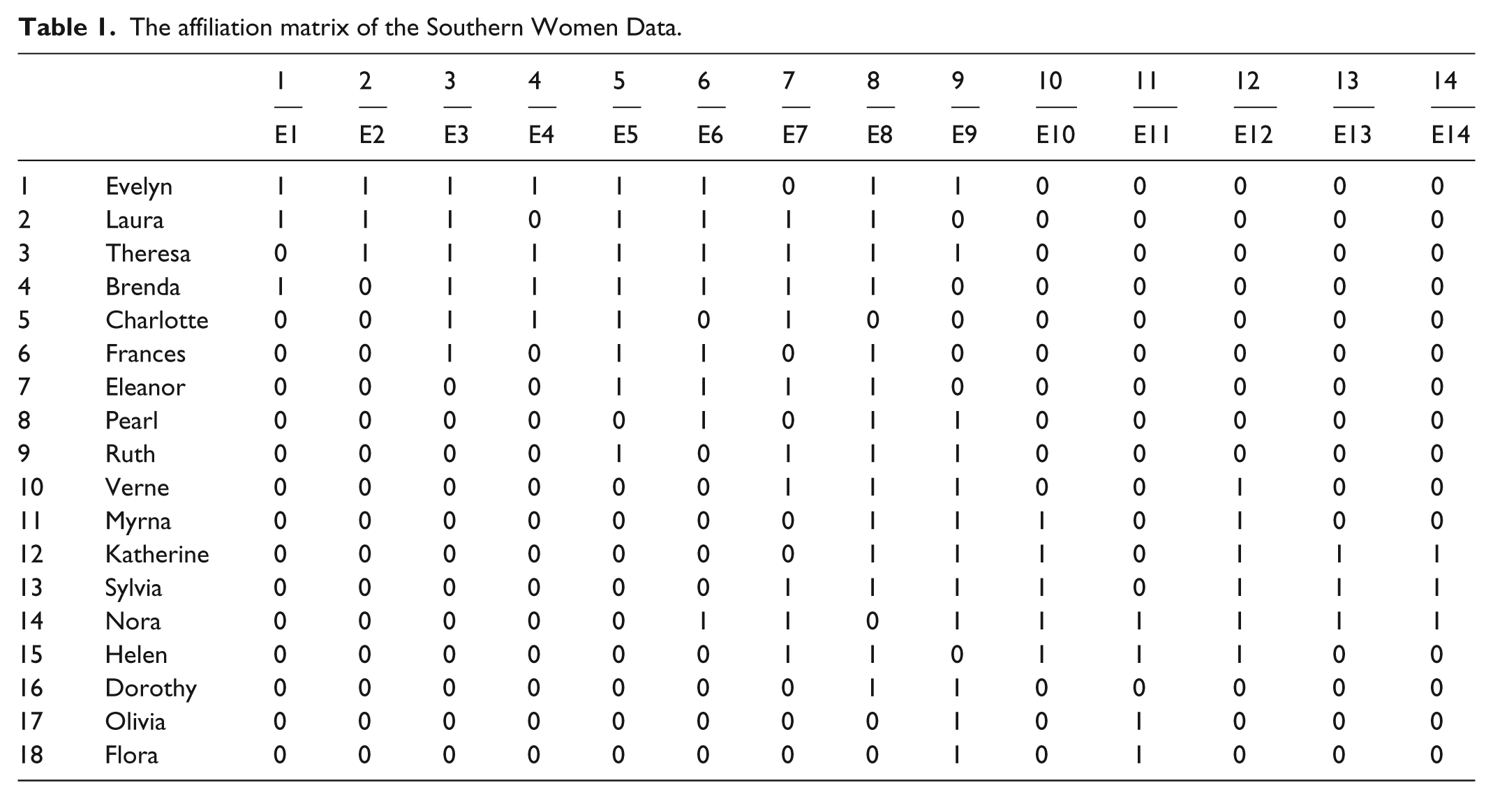
Two-mode social network data consist of two distinct sets of nodes, which we shall refer to as actors and events, together with a relation that connects actors to events. We require that there are no connections between actors, and no connections between events. Simple examples are groups of students and classes with the relation “attends.” Students attend classes and so there is a connection within the set of students or the set of classes. A second example is given by authors and journals where the relation is “has published in.” A classic example of this type of data is the Southern Women Data collected by Davis et al. (1941), in which they recorded the attendance of 18 women at 14 society events. Such data are often represented as an affiliation matrix, in which the rows are the actors and the columns are the events, and a 1 in row i column j means that actor i attended event j. Table 1 shows the affiliation matrix for the Southern Women Data.
The affiliation matrix of the Southern Women Data.
Data in this form are quite common in certain areas of application, for example, in studying interlocking directorates in which case the actors are directors and the events are boards of companies. Also, covert network data are often of this type, where the actors are say criminals and the events are crimes.
There have been two distinct approaches to analyze data of this form. The first is known as the projection method. The two-mode data are converted to one mode. For the actors, we can construct a matrix representing the relation “attended an event with.” Similarly for the events, we can construct a data matrix where the relation is “at least one woman attended both events.” We can go further and construct matrices which represent the number of times a pair of actors went to an event together and the number of actors two events have in common. These are given by the matrix products AAT and ATA, where A is the affiliation matrix and AT is the transpose of A. The relationship between these matrices was explored in a classic article by Breiger (1974). Once the projections have been constructed, then these are submitted to further analysis, often by first dichotomizing the projections. That is, converting them to a binary matrix by selecting a cut-off number values below which are set to zero.
The second approach is to analyze the two-mode data directly as a special kind of network. This approach was advocated by Borgatti and Everett (1997) and has until recently been the preferred method. The bipartite adjacency matrix B of an affiliation matrix A is given by
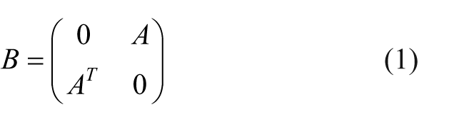
The matrix B is now a regular adjacency matrix in which the rows and columns have both the actors and the events. We can then submit B to standard social network methods. However, adjustments are needed to take account of the fact that there are no within mode relations, represented by the two zero blocks in equation (1). Examples of these adjustments are new normalizations for centrality measures and extensions of the clique concept to the bi-clique.
In a recent article, Everett and Borgatti (2013) proposed what they called the dual-projection approach. They suggested using both projections (undichotomized) analyzing and then combining the results of these using the original affiliation matrix A. They argue that if this approach is taken much of the criticism of projection, namely that data are lost in the process, is not valid. In their article, they explore this idea for core-periphery, structural equivalence and briefly centrality. Hence, if we were to use this for core-periphery, we proceed as follows. As a first step, construct the two one-mode projection matrices AAT and ATA. For the Southern Women Data, these matrices would be the woman-by-woman matrix in which the (i, j)th entries are the number of events woman i and woman j attended together; and the event by event matrix in which the (i, j)th entry is the number of women who attended both events i and j. These matrices are then submitted to the continuous core-periphery method to determine the core and peripheral events and the core and peripheral women. The results of these are then mapped back on to the original data matrix (as given in Table 1) to partition this single matrix. The process yields a core group of women (Evelyn, Laura, Theressa, Brenda, Nora, Eleanor, Ruth, Sylvia) and a core group of events (E5, E6, E7, E8, E9). The blocking shows the interactions between the core and peripheral women and the core and peripheral events.
Melamed (2014) looked at dual projection for community detection. Here, we will take a closer look at dual-projection centrality.
Dual-projection approach for centrality
In order to apply dual projection for centrality, we need to find the centrality of the actors in the projected actor-by-actor matrix and the centrality of the events in the projected event-by-event matrix. In order to use these scores, we need to make the actor centralities dependent on the event centralities they attend and the event centralities dependent on the actor centralities that attend the events. We note that the projection matrices are symmetric and valued. It follows that the only centrality methods we can use are ones that can be applied to valued data. Let r and c be the centrality scores of AAT and ATA, respectively, then the dual-projection method centrality “ac’ and “ec” scores are given by
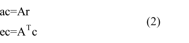
where “ac” is the actor centrality scores and “ec” is the event centrality.
One obvious centrality measure to consider for this approach is eigenvector centrality.
That is, the centrality given by the principal eigenvector of the projected matrices. This is exactly what Bonacich (1991) suggested in his article looking at eigenvector centrality for two-mode data. As Bonacich noted in this case, the centrality scores we obtain are exactly the same as the eigenvector centrality scores of the bipartite graph representation given in equation (1).
Given that using eigenvector as our underlying measure does not give us anything different, we instead will use flow betweenness (Freeman et al., 1991) as an example of this approach on the Southern Women Data. Flow betweenness is an example of a class of centrality measures called induced centrality measures. The idea is that we measure some property of the whole network, then delete a node, and see how much the measure changes and this is the centrality of the deleted node. In essence, it measures the extent to which an individual node contributes to the particular measure. For flow betweenness, this measure is the total amount of flow in the network. If we think of the value of the edges as the maximum capacity of the edge to carry something flowing through the network, then we can calculate the maximum possible flow between any pair of nodes. If we sum these maximum values for every pair of nodes, this gives us the total flow through the network. Hence, the flow betweenness centrality of a node is the change in total flow when it is deleted.
To calculate the dual-projection flow betweenness, we form the two projection matrices, calculate the two sets of flow betweenness to form r and c, then apply equation (2) to calculate the centralities. The results are given in Table 2 together with the standard flow betweenness of the bipartite representation, that is, the adjacency matrix B in equation (1). Column 1 is regular flow betweenness on the bipartite graph and column 2 is the dual-projection flow betweenness. All calculations were done using the software program UCINET (Borgatti et al., 2002).
Flow betweenness and dual-projection flow betweenness on the Southern Women Data.
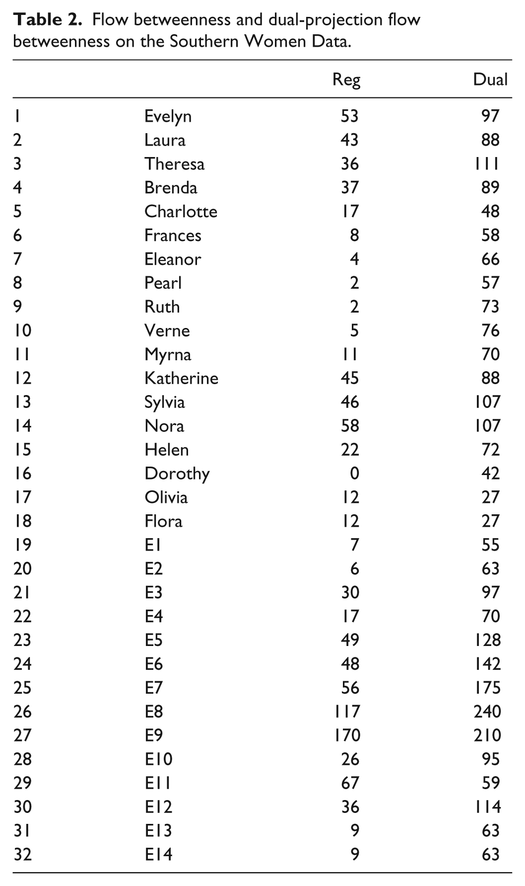
If we examine Table 2, we note that the actual scores for the dual projection are much higher than the standard flow betweenness on the raw data. Since the raw data are binary and the projected data are valued, then there will be an increase in the total. However, in comparing the columns, we should not directly compare values instead we are more concerned with the ordering. If we examine the top eight women in both methods, we see they are the same but with some differences in ordering. These eight women were identified as core in Everett and Borgatti’s core-periphery split of the women. Looking at the events, we again see that the events found to be core (E5, E6, E7, E8, E9) have the highest centrality scores for the dual-projection approach but not for the regular flow betweenness. This would suggest that the dual projection is superior to the standard flow betweenness at least for these data. In fact, we would expect the dual-projection method to outperform standard flow betweenness as the projected data are valued whereas the original data are binary. Flow betweenness is a method which requires valued data and so this in some respects is not a fair comparison.
As an alternative to validate the results, we can compare the dual-projection centrality score with the renormalized two-mode centrality scores for degree, closeness, betweenness, and eigenvector proposed in the article by Borgatti and Everett. These are given in Table 3.
Renormalized two-mode centrality scores for the Southern Women Data.
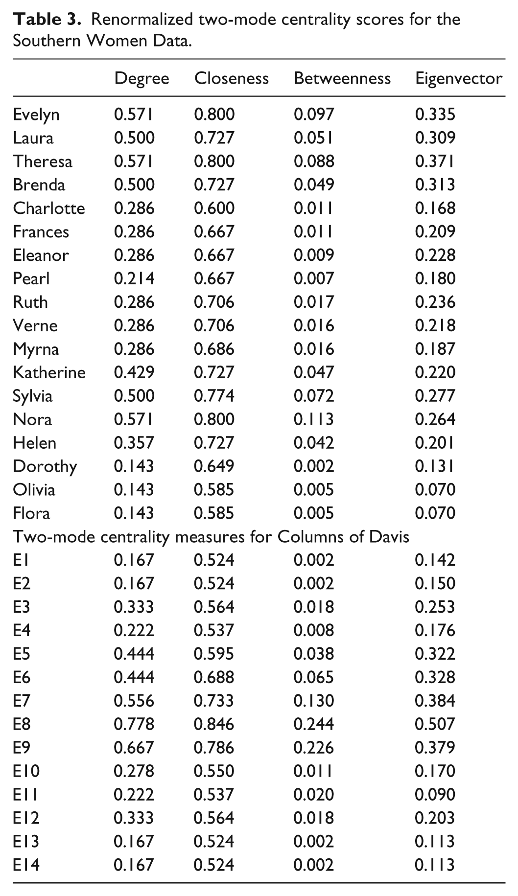
Overall, there is a great deal of similarity between most of the centrality scores. However, the scores that differ the most are again the flow betweenness on the bipartite network. We see, for example, that Theresa is ranked 5 on regular flow betweenness but is top in every other measure except two-mode betweenness where she is third. At the lower end of the women scores, we see that Dorothy, Flora, and Olivia are consistently at the bottom of the rankings except in flow betweenness where Flora and Olivia are replaced by Pearl and Ruth.
There is more consistency among the event scores where E1, E2, E13, and E14 have the lowest scores across the full spectrum of measures. At the top end, all measures except regular flow betweenness have E8 as the most central followed by E9 and E7. The high score given to E11 in regular flow betweenness is not reflected in any of the other centrality measures. These results provide further evidence of the superiority of dual-projection flow betweenness over applying flow betweenness directly on the bipartite network.
There are, however, some subtle differences between the dual-projection flow betweenness and the other methods which may be significant. For example, Sylvia has the second highest score in the dual approach (along with Nora) but is lower down the ranking in the other measures. Looking at the data, we see that Sylvia and Nora both attended three very central events (whereas most other core women attended four or more central events), but they were the only core actors attending the peripheral events E10 to E14. In this case, we might expect them to have a higher betweenness score than other women as they link women in the more peripheral events, a fact picked up for both of them in the dual-projection betweenness results.
One way to understand the differences and help select which method to use in other circumstances is to consider the nature of what flows through a network. This perspective was proposed by Borgatti (2005) for one-mode networks in his article on centrality and network flow. Degree is a local property and takes little account of the network structure. If we were interested in finding out what happened at the events and could interview just a few people, then clearly we would ask women with the highest degree centrality. Alternatively, we may see these women as the most gregarious or socially active in the network. Events with the highest degree may be seen to be the ones with the broadest appeal or the ones where it was important to be seen.
Alternatively, we may need to get a message as quickly as possible to all the actors in the network. In this instance, closeness would identify the individuals in the best position to do this. If instead of telling individuals, we wanted to make an announcement at an event, asking all those present to tell others, then the event closeness would identify the best event on which to do this. Instead of requiring all people to get the message as quickly as possible, we were more concerned that the well-connected people hear early in the process, then eigenvector centrality would be the best choice.
Different things flow through the network in different ways, information exists in many places at the same time. This is not the case for the movement of a physical object (say a book), and it follows that different processes are at work. The book moves from person to person and can only be in one place at one time. If I ask people to pass it on to a target in a small network, then it is likely to follow geodesic paths. The actor in the network who is able to control the flow of such objects to the greatest degree would be the one with the highest betweenness.
The descriptions above all assume that the flow of information or goods through the two-mode network is not constrained by the events. This would probably be true for the movement of important objects such pieces of crucial information but may not be true for lesser information such as gossip. The number of events two women attend together could be seen as the capacity to exchange information. Of course, they may or may not choose to exchange but it does measure the opportunity for exchange. This is precisely the values contained in the women-by-women projection matrix. The event-by-event projection matrix also gives the number of women attending pairs of events and again this could be seen as the capacity for exchange. It follows that the flow betweenness of the women measures the extent to which they can control the flow of things like gossip around the whole network. Note in this case, we do not restrict ourselves to shortest paths as we do with ordinary betweenness. The dual projection for flow betweenness takes into account the number of meetings the women have as well as the number of opportunities at each event. If this is seen as important, then this is the method that should be used.
As a second example of a dual-projection centrality, we look at the Bonacich (1987) power method. This method is closely related to the method first proposed by Katz (1953) and involves a parameter β. This parameter has to be less than the reciprocal of the largest eigenvalue. Fortunately, both AAT and ATA have the same eigenvalues and so we can select the same β for both projections. The reciprocal of the largest eigenvalue for the projected Davis data is 0.022. We do not want to select a value close to this as this would produce results that are very similar to eigenvector centrality and so we choose 0.01 as our value of β. We also ran Bonnacich power on the bipartite network; in this case, the reciprocal of the largest eigenvalue was 0.14. As we had taken the midpoint in the dual projection, we selected 0.07 for the bipartite as a comparison. The results are shown in Table 4 where column 1 is the regular Bonacich power and column 2 is the dual-projection power.
Bonacich power for the Southern Women Data.
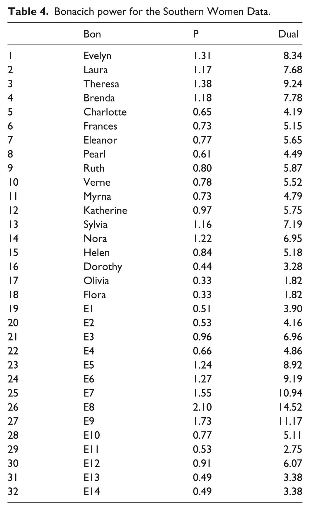
The ordering of the events is almost identical between the dual projection and the bipartite approach with just E11 in a different order. The ordering of the women is also similar with just a few marginal differences and also in broad agreement with the results from Table 3.
So far we have obtained results from the dual-mode projection that are almost the same as those obtained from other techniques. We give as a final example one in which the results differ. We first recall that Bonacich suggested that the beta value for his measure could be negative, reflecting the fact that it is not always good to be connected to highly connected actors. The classic example of this is in exchange networks. If an actor x has many choices with whom to trade goods, but each of these only has the option of trading with x, then x is in a good position and all of x’s alters are in a weak position.
We now explore how this can be conceptualized for the Southern Women. In which case we have to consider a situation when it is not good to go to popular events. Let us suppose that the women want to be noticed at events, but at events that lots of women attend there will be much competition and so lowering the chances of being noticed. It follows in this case that it is not good to go attend the popular events. This can be captured using a negative beta on the bipartite representation and would not need a dual-projection approach.
Suppose instead a woman wanted to expand her social circle. In this case, approaching a woman who has many contacts with other women may not be as useful as making contact with a woman who has few contacts. The woman with many contacts may not feel she needs or has time for any new relationships and may see forming a relationship with someone with few friends as detrimental. In this case, it is better for a woman seeking to expand her circle to be at events in which the other women are in the same situation. In which case, it is important to attend events in which the other attendees have been to a small number of events with other women. In this case, it is not how many women were at the event, but how many events they attend with other women is important. This will not be picked up from the bipartite representation but should be picked up by the dual-projection method.
There is an added complication with using a negative beta on the bipartite network. Bonacich’s methods with negative beta subtract the weighted counts of walks of even length from the count of walks with odd lengths. The even length walks will only connect women and events but the odd length walks will connect women with women and events with events. One consequence of this is that larger values of beta result in positive and negative centrality scores and it is not clear how these should be interpreted. In our implementation, we have selected the largest negative beta that gives positive centrality scores. For the bipartite representation, β is set at −0.09 and for the dual projection, −0.02. The results are given in Table 5.
Bipartite and dual projection using Bonacich power with negative beta.
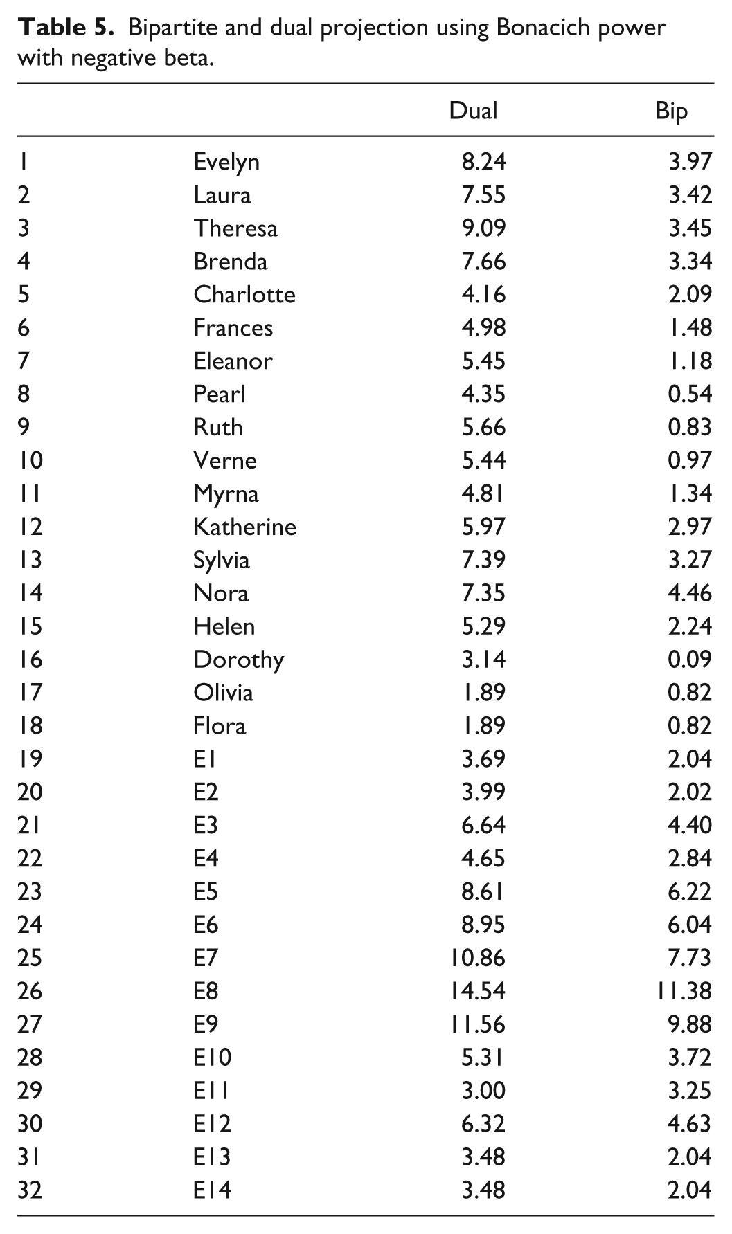
We can see that three women, namely Nora, Ruth, and Charlotte move five or more places in the rank ordering between the methods. We focus our attention on Charlotte and we see she is ranked 15th in the dual projection with just Dorothy, Olivia, and Flora below her. In the bipartite method, Charlotte is ranked six places higher in 9th position. We can see that Charlotte attended four events, three of which were smaller events (E3, E4, E5) and one, E7, was a larger event. This is much better than women such as Dorothy, who attended just two large events but not as good as women such as Evelyn who attended five small events and three large events. This places Charlotte around the middle of the rankings using the bipartite method. To see why Charlotte was placed so low in the dual projection, we examine the women-by-women projection matrix. Figure 1 shows the women-by-women projection matrix dichotomized at level 4. Hence, it shows an edge between two women if they attended four or more events together.
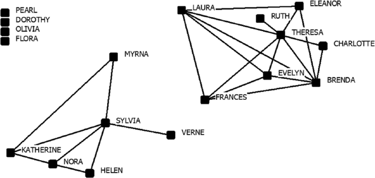
Projected women dichotomized at level 4.
In Figure 1, we see that Charlotte has just two connections to two women Brenda and Theresa, both of whom have many connections. As a consequence, Charlotte’s centrality is quite low in the dual-projection approach. The dual projection does not just use information from the women-by-women matrix but also uses the event-by-event matrix and so this should not be seen in isolation. However, we see that the Event scores are far more stable between the two methods with only E2 and E11 changing positions by more than one place and these do not affect Charlotte as she was not involved with these events. An examination of both Nora and Ruth as well as events E2 and E11 show similar reasons for the changes in ranking.
Conclusion
In their article, Everett and Borgatti (2013) suggested that it would be possible to use other centrality measures in their dual-projection approach. They acknowledged that eigenvector centrality could be used but that this was exactly what Bonnacich had done in his 1991 article. In order for a centrality method to be able to be used in dual projection, it must be applicable to valued data. As Everett and Borgatti point out degree centrality is a candidate, but the way the dual projection is set up using degree would result in similar results to eigenvector. The reason for this is that in using the dual projection method for degree, it replicates the first few iterations of the power method for finding eigenvectors, and hence would produce very similar results. In order to test their approach, we first used flow betweenness comparing the results of the dual projection with the bipartite approach. We also compared results with other centrality measures for two-mode data and found a great deal of consistency. As a second method, we examined Bonacich’s power method. This again showed a high level of consistency with the bipartite method for positive beta. However, when we examined taking negative values of beta, we saw some differences in the results. These differences were entirely interpretable and consistent with what the method was designed to do and so can be seen to extend the methodological tool kit for analyzing two-mode data.
The main purpose of this article was to show that dual-projection centrality is a viable tool capable of providing additional insights into the structure of data. We feel this has been achieved and this paves the way to look at additional centrality measures for valued data.
In addition, by examining possible processes that may be at work in the network, we have shown how appropriate measures can be selected. We argued that if event size was important then the direct method was appropriate but if the properties of the attendees were more important, then the dual-projection approach would be a better method. Selection of a centrality measure needs to take account of the underlying assumptions the measure makes. It is often convenience that dictates what measures are used rather than a careful selection based on the underlying principles of the measure. Care needs to be taken in selection and interpretation and this requires careful analysis when using dual projection.
We examined a few of the potential measures that could be used in a dual-projection approach. Recently, Opsahl et al. (2010) suggested classes of measures for valued data including new degree, closeness, and betweenness formulations and these could also be used. There is now a large class of centrality measures with more being developed all the time. Any measure that can be applied to valued (undirected) data can be used in a dual-projection formulation. The challenge now is to see which of them bring understanding and insight to substantive problems.
Footnotes
Declaration of conflicting interests
The author(s) declared no potential conflicts of interest with respect to the research, authorship, and/or publication of this article.
Funding
The author(s) received no financial support for the research, authorship, and/or publication of this article.