
Abstract
This article demonstrates the innovative use of the log-linear distance model in the assessment of homophily in a set of small groups, such as the co-participants in a set of events. It traces the development of the application of the log-linear distance model to the study of homophily and reviews its recent use to assess the extent and structure of gender and age homophily in groups of criminal accomplices (‘co-offenders’). The transformations of the group membership data that are a prerequisite of the log-linear analysis, and the interpretation of the log-linear parameters, are explained in detail in order to make the approach accessible to potential users. Although the described applications are to gender and age homophily in groups of criminal accomplices, the method can be used to assess homophily on one or more variables in any small groups.
Homophily – the tendency to associate with others who are similar to oneself – is ubiquitous in social relations (McPherson et al., 2001). Recently, the log-linear distance model has been used innovatively to model homophily on ordinal and dichotomous variables in small groups of criminal accomplices (Carrington, 2015a, 2015b); however, the methods are equally applicable to any small groups. Although the methods are introduced in the cited sources, their explanation of the methods is very brief. This article explains the methods in detail. It discusses the conceptualisation and operationalisation of homophily, traces the development of the application of the log-linear distance model to homophily and its advantages over the well-known Coleman index, shows how it can be applied to small groups and reviews the recent applications (Carrington, 2015a, 2015b). No new results are reported: the purpose of this article is to put the recent applications in conceptual and historical context and to make the model accessible to potential users.
Conceptualising homophily
Homophily has been defined as ‘the principle that a contact between similar people occurs at a higher rate than among dissimilar people’ (McPherson et al., 2001: 416). Mayhew et al. (1995) characterise homophily as ‘the social distance interaction hypothesis’: ‘The frequency with which people enter into face-to-face association (contact, interaction) is inversely related to the social distance between them’ (p. 20). Thus, according to the principle, or hypothesis, of homophily, the highest rate of interaction is expected between people who are in the same category of a discrete variable (e.g. both male) or who have the same value on a continuous variable (e.g. same age), that is, whose social distance is zero.
As the definition of McPherson et al. (2001) implies, the phenomenon of observed homophily, or homogeneity in social relationships, does not in itself imply any particular explanation. In particular, it is not necessarily due to personal choice (Mayhew et al., 1995: 20). Explanations of observed homophily generally fall into three categories:
Population composition: This might be characterised as the ‘null’ hypothesis. The selection of interaction partners is influenced simply by the availability of potential partners. If partners are selected at random, then their characteristics will reflect the distribution of those characteristics in the population or pool of potential partners. If the population is distributed unevenly over categories or values of some attribute, then – assuming random selection of partners –members of the numerical majority group(s) will be more likely to select similar partners, and homophily will be observed (Blau, 1977). 1 McPherson et al. (2001: 419) refer to this as baseline homophily. For example, because the great majority of criminals are male, random (i.e. gender-blind) selection of accomplices would, ceteris paribus, produce a high proportion of homophilous male co-offending groups (and a smaller number of mixed-gender and all-female groups), and that is precisely what has been observed in numerous studies of co-offending (van Mastrigt and Carrington, 2014).
Preference: For various reasons, people prefer to associate and collaborate with those who are similar to them. According to McPherson et al. (2001), ‘the psychology literature has demonstrated experimentally that attraction is affected by perceived similarity …’ (p. 435). Similarly, in the area of professional collaboration, Steffensmeier and Terry (1986) concluded on the basis of interviews with male thieves that they preferred same-gender accomplices because they were perceived as more reliable and trustworthy.
Social structure: Features of the social structure apart from overall population composition may constitute ‘opportunity structures’ that favour homophilous contact and collaboration. For example, McPherson et al. (2001) point out that ‘organizational foci’, such as neighbourhood play groups, schools, workplaces and voluntary organisations, bring together people who are similar in age, ethnicity, socioeconomic status and sometimes gender (pp. 431–434). Felson (2003) describes ‘convergence settings’, where local youth ‘hang out’ and have the opportunity to meet and screen potential criminal accomplices. Such ‘opportunity [to meet and screen] structures’ are often partly or entirely segregated by age, gender, ethnicity and so on, thus restricting the pools of potential partners to similar people. Waring (2002), Schwartz et al. (2015) and others (reviewed in van Mastrigt and Carrington, 2014) have noted that it is the ‘local’ availability and accessibility of potential criminal partners, rather than their distribution in the larger population, that affect partner selection and that local availability and accessibility are structured by social networks based on family, friendship, neighbourhood and so on. Pettersson (2003) shows that residential ethnic segregation leads to ethnic segregation (homophily) in co-offending, although individual preferences may tend towards ethnic heterogeneity.
As the ‘baseline’ homophily that can be accounted for by random selection and population composition is often of little theoretical or substantive interest, 2 some researchers restrict the definition and study of homophily to that which exceeds expectations under random selection – sometimes termed inbreeding bias or inbreeding homophily (Coleman 1958; Currarini et al., 2009; Currarini and Redondo, 2011; Fararo and Sunshine, 1964; Laumann and Pappi, 1976: 55; McPherson et al., 2001: 419; Marsden, 1988; van Mastrigt and Carrington, 2014). For example, Coleman (1958: Appendix B) conceptualises homophily in sociometric choices as the extent to which the number of actual choices of persons in the same category as the chooser exceeds the number expected under random selection. Coleman’s (1958: 36) index of homophily is category-specific
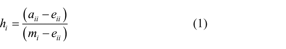
where hi is the (inbreeding) homophily of persons in category i, aii is the number of same-category choices made by members of category i, mi is the total number of choices made by persons in category i and eii is the expected number of same-category choices by persons in category i, under random selection, which is equal to mi multiplied by the proportion of persons of category i in the population.
Limitations of the Coleman index
Although the Coleman index of inbreeding homophily has been used extensively (for recent applications, see, for example, Currarini et al., 2009; Currarini and Redondo, 2011; van Mastrigt and Carrington, 2014), it has several limitations:
It is based on a binary conceptualisation of similarity: persons chosen are either of the same category or not. This can be seen in formula (1). Therefore, its application is limited to dichotomous variables or to polytomous variables that can be analysed as dichotomies. The notion of social distance – other than ‘same/different’ – is unknown.
The estimate of homophily that it produces is category-specific. No overall estimate of homophily in the population is available.
Its sampling distribution is unknown, so there is no known standard error and therefore no inferential statistics such as confidence intervals or significance tests.
It is not readily incorporated into a multivariate model, in which, for example, homophily can be assessed while controlling other relevant variables.
The log-linear distance model
The limitations of the Coleman index of homophily do not apply to the log-linear distance model. It applies to ordinal (and dichotomous) variables, it has a well-understood sampling distribution and therefore a standard error, from which confidence intervals and significance tests can be derived, and it is part of the statistically well-developed and well-understood log-linear model and, more generally, of the generalised linear model (Agresti, 2013: Chapters 9–11).
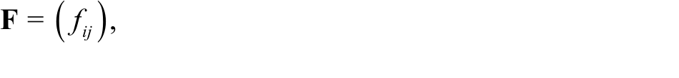
The simplest log-linear distance model is applied to a square cross-tabulation
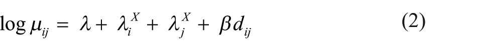
where µij is the count (i.e. frequency of dyads) in cell (i, j), X is the row and column variable, indexed by i (rows) and j (columns) and
Like all conventional log-linear models for two-way tables, the distance model includes an intercept parameter λ, parameterising the overall frequency,
3
and row and column parameters
Development
The log-linear distance model was introduced by Goodman (1972, 1979: model 7, p. 810; see also Breiger, 1981; Haberman, 1974) 5 for square ordinal social mobility tables, in which cell counts (i, j) indicate the number of father–son dyads for which father is in the ith occupational class and son is in the jth occupational class. Cells on the main diagonal – where i = j and father and son are in the same occupational class – indicate social immobility (‘status inheritance’; i.e. inheritance by a son of his father’s occupational class); cells at increasing distances from the main diagonal indicate increasing amounts of upward or downward social mobility. The β parameter (in model 2 above) captures the strength of the association between the number of occupational classes (|i − j|) separating father and son and the number of father–son dyads in cell (i, j), that is, the extent to which social mobility exceeds expectations based on random placement of sons in occupational classes.
Marsden (1988) applied the log-linear distance model to analyse homophily in personal networks. The 1985 American General Social Survey captured data on the characteristics of up to five persons with whom respondent ‘discussed important matters’. Marsden (1988) transformed the data into (up to) five respondent–alter dyads for each respondent and then constructed cross-tabulations – on age, education, race/ethnicity, religion and gender – with rows representing respondents, columns representing alters and counts of dyads in the cells. Various forms of the log-linear distance model were applied to these cross-tabulations in order to assess the amount and structure of homophily on each attribute of respondents’ choices of discussion partners.
Extension to small groups
The log-linear distance model applies to a cross-tabulation of dyadic interactions: the categories of the variable to which the two members of the dyad belong are indexed in the rows and columns of the cross-tabulation. Therefore, it is inapplicable to interactions involving more than two actors and therefore to groups of more than two members.
6
However, any ‘small’ or ‘face-to-face’ group incorporates a set of dyadic, or pair-wise, interactions or relationships: a group of size n generates n(n − 1)/2 dyads (Mayhew et al., 1995: 25–27). This phenomenon is limited to ‘small’ groups because in larger groups it is unrealistic to assume that all members interact with all other members (Mayhew et al., 1995: 25). As Schaefer (2012) writes, in justifying the omission of larger groups from a study of social versus spatial distance in criminal collaborations,
The assumption is made that individuals who were part of the same offense [i.e. co-offending group] had a social relationship. Two offenses were dropped from the data because they had such a high number of participants (23 and 54) that they likely violated this assumption. (p. 143)
Stegbauer and Rausch (2012) showed how lists of the members of a set of small groups of varying sizes can be used to generate a cross-tabulation of co-participating dyads, without knowledge of the identities of the members. Specifically, they transformed a list of the nationalities of the co-participants in a set of events (namely, sessions at an academic conference) into a set of co-participating dyads, labelled by the nationalities of the members, which in turn were used to generate a cross-tabulation of the frequencies with which people of different (and the same) nationalities co-participated in conference sessions. As nationality is a polytomous nominal variable, the concept of social distance was inapplicable, as was the log-linear distance model.
Carrington (2015b) extended the method of Stegbauer and Rausch (2012) to analyse age homophily among co-offenders (accomplices in crimes) apprehended by police in connection with all recorded co-offences in Canadian police during 2006–2009. Like Stegbauer and Rausch (2012), Carrington (2015b) began with information on one characteristic of each of the co-participants in a set of events: specifically, the age in years of each of the offenders. The distance model was particularly appropriate because age (unlike nationality in the research of Stegbauer and Rausch, 2012) is an ordered attribute and was coded in the data as an ordinal variable, with values from 3 to 88 years. The co-offences in the data ranged in size (i.e. number of recorded participants) from 2 to 44 co-offenders, but the great majority had only 2 or 3 co-offenders.
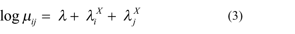
Following the method of Stegbauer and Rausch (2012), Carrington (2015b) created a square symmetric cross-tabulation with 86 rows and columns, representing ages from 3 to 88 inclusive. Cell counts (i, j) indicated the number of co-offending dyads in which a person aged i + 2 co-offended with a person aged j + 2. Formally, the age-by-age co-offending matrix is
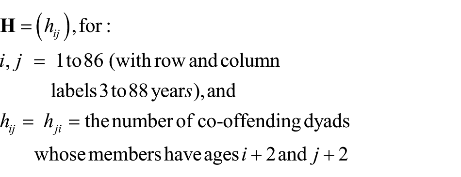
The matrix
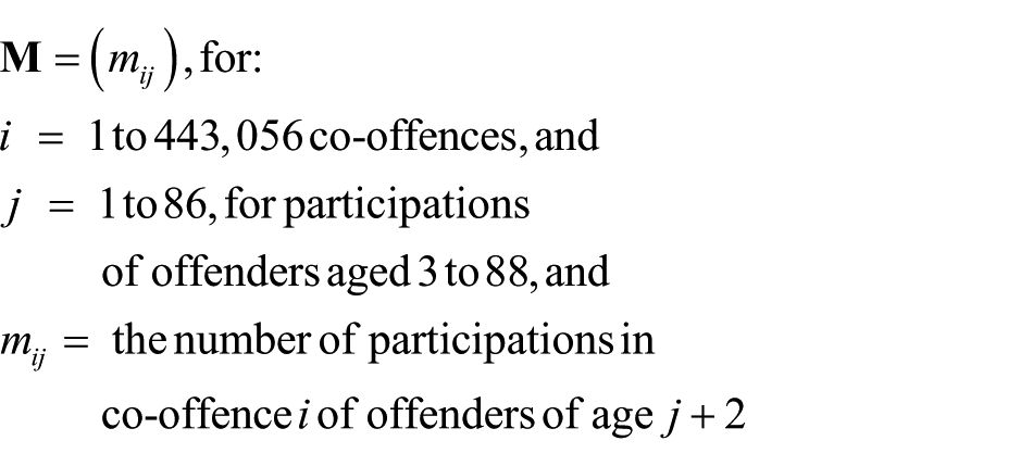
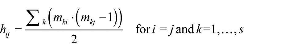
For example, Figure 1(a) shows three hypothetical co-offences labelled A, B and C, involving nine co-offenders aged 3–7 years. The first co-offence has five co-offenders, of whom two are 3 years old, and one each is 5, 6 and 7 years old. This co-offence comprises 10 co-offending dyads: Jack–Joe, Jack–Harry, Jack–Walter, Jack–Mac, Joe–Harry and so on The second and third co-offences have only two co-offenders each and therefore comprise only one co-offending dyad each; in the second, they are both 4 years old, and in the third, they are 5 and 6 years old. Figure 1(b) shows the resulting rows of the incidence matrix
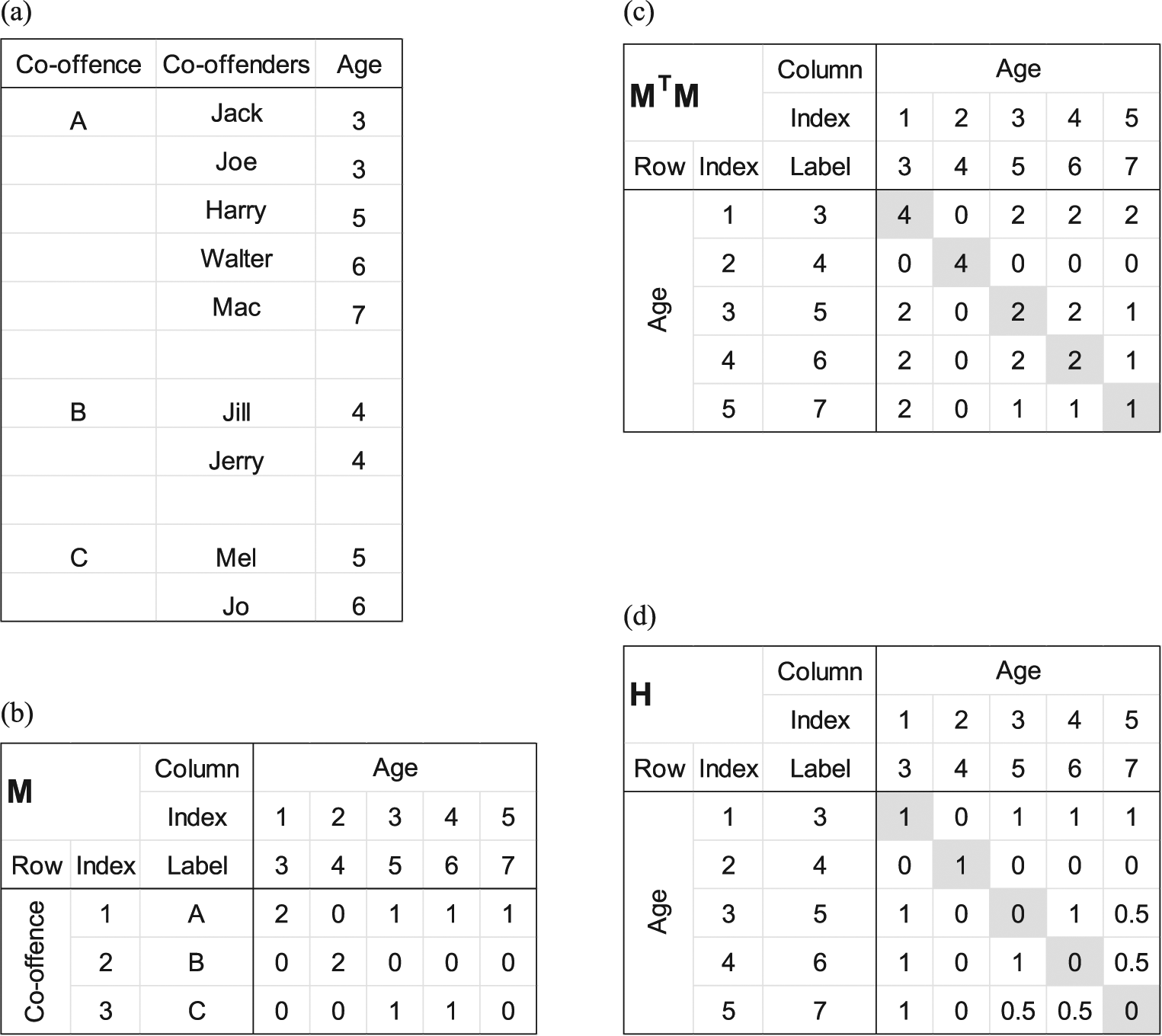
Transformation of co-offending data into an age-by-age matrix: (a) co-offending data, (b) weighted incidence matrix
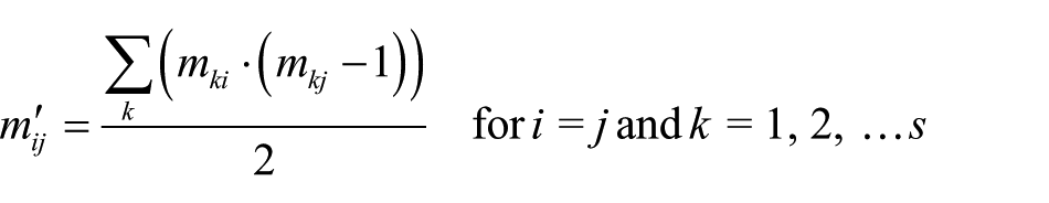
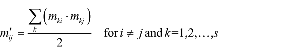
When
where s is the number of rows in
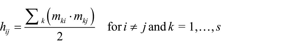
where s is the number of rows in
The age-by-age matrix
where µij is the count (i.e. frequency of interactions) in cell (i, j) and X is the row and column variable, indexed by i and j.
The marginals can be plotted in an age-by-age matrix (Figure 2). In Figure 2, the density of the shading of cells is proportional to the normalised residual. As predicted by the homophily hypothesis, co-offending is greater than expected (from population composition) on and near the main diagonal (red cells) and less than expected off the diagonal (green cells). This is confirmed by the distance parameter estimate β from the log-linear distance model (formula (2)), which was −0.1398 (standard error (SE) = 0.0002, p < 0.0001): that is, negative and statistically significant (Carrington, 2015b: 345–346).
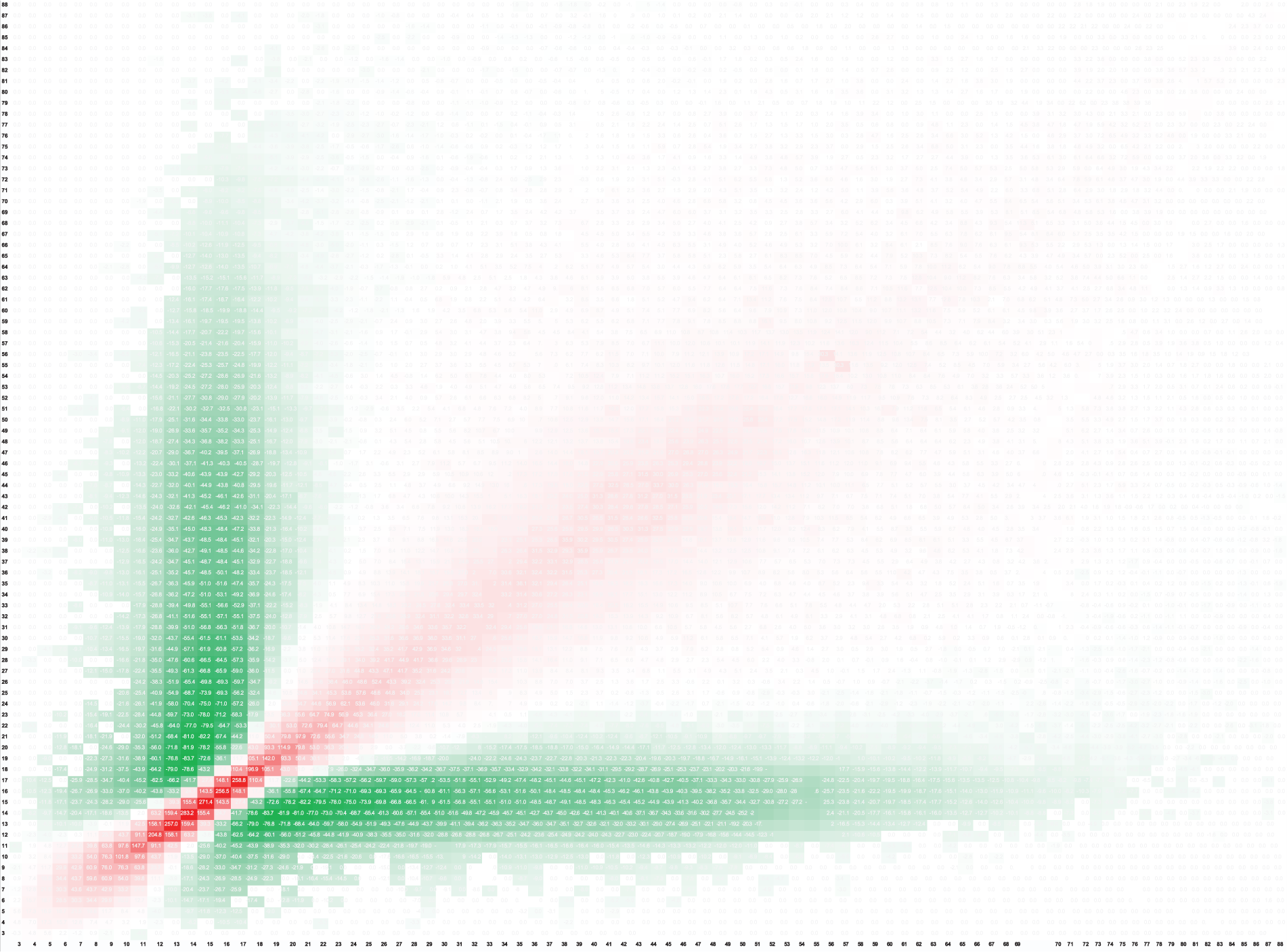
Age-by-age cross-tabulation with row and column marginal effects removed (residuals from the independence model).
Further hypotheses based on age-by-age cross-tabulation were tested in Carrington (2015b), primarily concerning variations in homophily with co-offenders’ ages – which can be seen in Figure 2, where homophily appears to be stronger among teenagers and children and practically non-existent among older co-offenders. This phenomenon was modelled by the ‘variable distance’ model, which allows the effect of social distance to vary
where d = |i − j| and s = i + j (Carrington, 2015b: formula 2, p. 345).
The β2 parameter represents an interaction between heterophily and age; a positive estimate for β2 indicates that age heterophily increases – that is, age homophily decreases – with an increase in the sum of the ages of the members of the dyad. Carrington (2015b) also tested hypotheses and models that added social distance based on age groups to distance based on year of age. The concept of ‘age group’ and models for it are discussed in the following section.
Extension to two variables
Carrington (2015a) extended the approach of Carrington (2015b) to model homophily on two variables (gender and age) simultaneously. Homophily on each variable was estimated while controlling for homophily on the other variable (as well as for population composition), and the interaction between homophily on the two variables was estimated: that is, whether or not co-offending between occupants of certain pairs of categories of the two variables occurred more or less frequently than expected on the basis of homophily on each of the variables individually.
Carrington (2015a) used the same data as Carrington (2015b), but the age range was trimmed to 5–75 years in order to have at least 10 female co-offenders for each year of age. The result was a reduction to 968,712 co-offending dyads. As with Stegbauer and Rausch (2012) and Carrington (2015b), the dyads were transformed into a cross-tabulation, but in this case it was a four-dimensional 71 × 71 × 2 × 2 cross-tabulation by age and gender simultaneously:
where i, j = {1, 2, … 71}, labelled by ages {5, 6, … 75}; k, l = {1, 2}, labelled by {‘Male’, ‘Female’}; and hijkl = hjilk ≡ the number of co-offending dyads whose members have the ages indexed by i and j and genders indexed by k and l.
To transform the individual co-offending groups into dyads, they were first transformed into two weighted incidence matrices
where i = {1, 2, … , 442,534}, indexing co-offences; j = {1, 2, … , 71}, indexing participations of male offenders with ages 5, 6, …, 75; and mij = the number of participations in co-offence i of male offenders of age j.
where i = {1, 2, … , 442,534}, indexing co-offences, j = {1, 2, … , 71}, indexing participations of female offenders with ages 5, 6, … ,75, and fij = the number of participations in co-offence i of female offenders of age j.
For example, Figure 3(a) shows three co-offences labelled A, B and C, involving nine co-offenders aged 5–9 years. The first co-offence has five co-offenders, all male, of whom two are 5 years old and one each is 7, 8 and 9 years old. This co-offence generates 10 co-offending dyads. The second and third co-offences have only two co-offenders each and generate one dyad each; in the second co-offence, they are both 6 years old and of different genders, and in the third co-offence, they are 7 and 8 years old and of different genders. Figure 3(b) shows the resulting incidence matrices
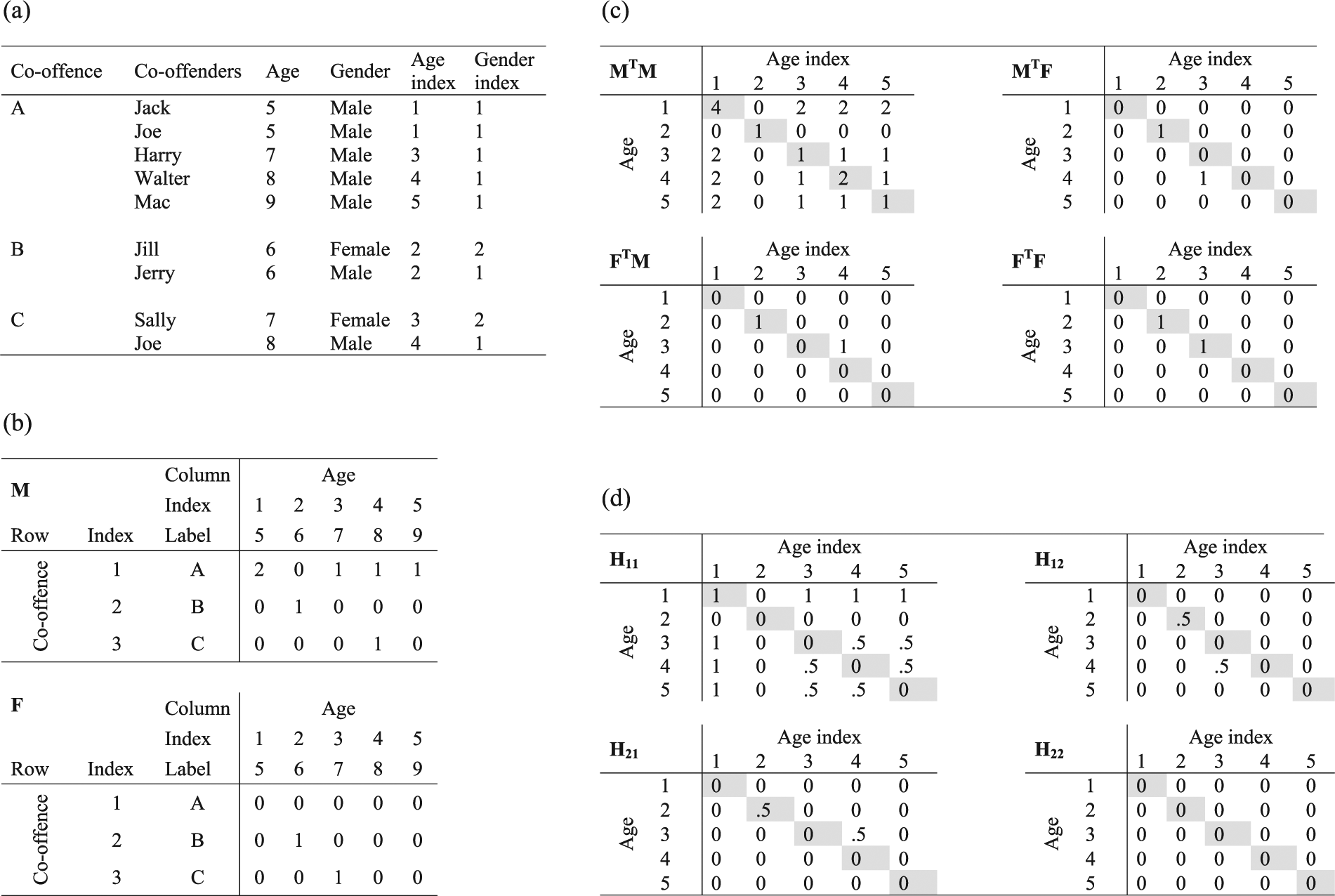
Transformation of co-offending groups to cross-tabulated dyads: (a) co-offending data, (b) weighted co-offending incidence matrices, (c) adjacency matrices with uncorrected cell counts and (d) the four slices of the four-dimensional cross-tabulation, with corrected cell counts.
When
where s is the number of rows in
As in Carrington (2015b; see preceding section), a further correction was required, because the entire symmetric matrix was analysed, unlike the analysis in Stegbauer and Rausch (2012), where only the lower triangle was analysed. In
where s is the number of rows in
The same procedure was followed to produce the female*female co-offending adjacency matrix
The 71 × 71 × 2 × 2 cross-tabulation of co-offending dyads was then reduced to a 3 × 3 × 2 × 2 cross-tabulation by aggregating years of age into age statuses, which Carrington (2015a) argues are more sociologically and criminologically relevant than merely chronological years of age or the ad hoc groupings of ages into ‘age groups’ in Carrington (2015b). Following Burt (1991), dyadic co-offending frequencies were row- and column-normalised using iterative proportional fitting (IPF), 8 in order to remove the effects of varying volumes of co-offending by members of different year-of-age groups. Distances (dissimilarities) between the co-offending patterns of each pair of years-of-age were calculated as the Euclidean distance between the corresponding pair of rows (or, equivalently, columns) in the two-dimensional 71 × 71 year-of-age by year-of-age cross-tabulation of normalised co-offending frequencies (Burt, 1991). Two methods were used to cluster the years of age in the resulting 71 × 71 distance matrix: visual examination of a multidimensional scaling (MDS) plot and Ward’s hierarchical agglomerative clustering method. 9 For Ward’s clustering, the choice of the number of clusters was assisted by plots of the pseudo-F statistic and pseudo-t2 statistic against the number of clusters (Cooper and Milligan, 1988). Ward’s clustering solution suggested either three clusters − 5–11, 12–17 and 18–75 years – or four clusters, with 18–75 years split into 18–45 and 46–75 years. The MDS plot (Figure 4) suggests (the same) three age clusters: 5–11, 12–17 and 18–75 years. Although derived from a clustering based on (dis-)similarities in co-offending patterns, these age clusters correspond exactly to the three age categories defined in Canadian criminal law: children (5–11 years), who cannot be prosecuted for criminal offences; youth (12–17 years), who are under the jurisdiction of the youth justice system; and adults, who are under the jurisdiction of the ordinary criminal justice system (Carrington, 2015a). 10
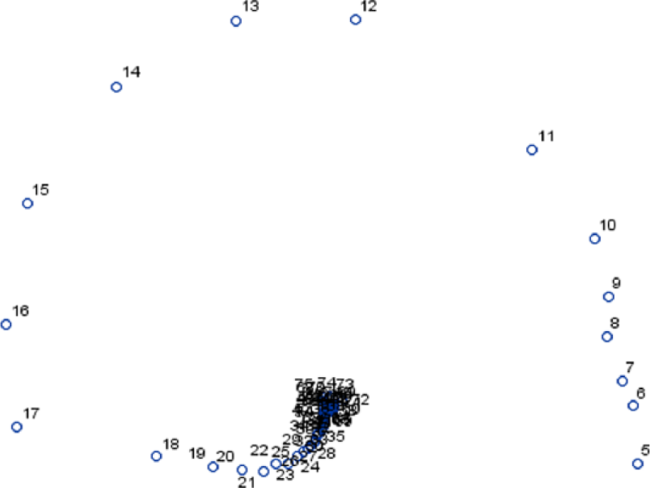
Two-dimensional MDS plot of distances between years-of-age, based on co-offending patterns.
The estimates for the gender and age status heterophily parameters were both negative and statistically significant (−0.757 and −1.897, respectively), indicating gender homophily and even stronger age status homophily among the co-offenders. The estimate for the interaction between gender and age status was 0.323 (SE = 0.008, p < 0.0001), indicating that dyads comprising a young female and an adult male are more frequent than expected from the main effects of gender and age, that is, gender and age status homophily are mutually attenuating, not reinforcing (Carrington, 2015a).
Limitations
The log-linear model of homophily in groups is a ‘dyad-independent’ model that assumes there are no connections between groups (Handcock et al., 2008). Where data are available on connections between groups – that is, if information is available on the presence of the same persons in two or more groups – then a model such as the exponential random graph model (ERGM) is, in principle, more appropriate because it can estimate homophily (using the same underlying distance model) while controlling for network effects (Robins and Daraganova, 2013: 93). However, there are limitations to the size of population that can be modelled with an ERGM (Robins and Lusher, 2013), whereas the approach described here is insensitive to population size, as the nodes are aggregated into categories of the classificatory variable.
The log-linear distance model also has the limitation that the transformation of groups into dyads, preparatory to construction of the cross-tabulation required by the log-linear model, loses information about group size. As homophily has been found to be related to group size (McPherson et al., 2001; Mayhew et al., 1995; van Mastrigt and Carrington, 2014), this may be an issue in some applications.
Conclusion
The log-linear distance model is a powerful and flexible way of modelling inbreeding homophily in small disconnected groups on attributes measured with ordinal or dichotomous variables. It brings the modelling of homophily into the overall family of log-linear models, whose statistical properties are well-known and whose parameterizations are extremely flexible and therefore readily adaptable to the testing of specific hypotheses. In order to apply the log-linear model to data on group memberships, the list of the members of each group must first be converted to a cross-tabulation of dyadic relationships, following the method of Stegbauer and Rausch (2012). Examples of the use of the log-linear distance model to assess age and gender homophily in co-offending groups are provided in recent work by Carrington (2015a, 2015b).
Footnotes
Acknowledgements
The author gratefully acknowledges the continuing support of the Canadian Centre for Justice Statistics, Statistics Canada for this programme of research and thanks Yvan Clermont, Julie McAuley, Anthony Matarazzo and Marian Radulescu for their assistance in accessing the data. The article has benefited from comments on earlier versions by Ronald Breiger, John Scott and an anonymous referee The opinions expressed herein are those of the author alone and do not represent the opinions of Statistics Canada.
Declaration of conflicting interests
The author(s) declared no potential conflicts of interest with respect to the research, authorship and/or publication of this article.
Funding
The research was supported by a grant from the Social Sciences and Humanities Research Council of Canada.