
Abstract
Timbral blend is fundamental in various musical activities for shaping sounds and musical intentions. Previous studies on blend perception have mostly focused on sounding blends, neglecting imagined blend made possible by inner hearing where sounds are imagined in the mind. Experiment 1 investigated how imagined blend compares to the perception of heard blend and whether musical background has an effect. Two groups of participants (musicians and nonmusicians; N = 31 per group) were presented with pairs of short instrument sounds in unison from 14 different instruments in two different experimental conditions. In the first condition, paired sounds were played sequentially, and participants were instructed to imagine them being played simultaneously and to rate their degree of blend. In the second condition, pairs of instrument sounds were played simultaneously, and participants were asked to rate the perceived degree of blend. Results showed significant interaction effects among the instrument pairs, presentation conditions, and musical backgrounds. Acoustic modeling and multidimensional scaling of blend ratings showed both varying and invariant roles of different acoustic features between the two types of blend perception. Imagining blend appears to be more sensitive to differences in brightness and richness of the high partial content between the blending sounds. Experiment 2 with 48 participants was conducted on the perception of dissimilarity between instruments, using the same stimuli as the previous experiment. Results from this experiment provided evidence that evaluating imagined blends is strongly informed by judging the dissimilarity of blending instruments. In practice, how the two types of blends differ is a result of complex interactions involving the specificity of blending instruments and listeners’ musical backgrounds.
Keywords
The perceptual complexity of timbre has been well described in the existing literature in both music theory and psychophysics. As timbre is a property of fused auditory events (Siedenburg & McAdams, 2017a), it is of natural interest to investigate the operational aspect of creating new timbres from different sonic constituents, examining how distinct sound sources fuse into a single perceptual unity or remain separated. In the case of fusion, the resulting composite sound creates the illusion of a “virtual source image” (McAdams, 1984, p. 289). Fused concurrent sounds can have a range of distinct timbral characteristics (Sandell, 1995), which offer great potential for orchestration and composition in the form of different instrumental combinations. Unsurprisingly, orchestration treatises have given great attention to the choices of concurrent combinations of different instruments for achieving different sonic intentions (e.g., Adler, 2002; Berlioz & Strauss, 1948; Read, 2004; Rimsky-Korsakov, 1964). Various psychoacoustic studies have also focused on the perception of concurrent instrumental sounds (for a recent review on this, see McAdams, 2019), many of which have specifically dealt with the perception of blend of concurrent timbres and its potential acoustic correlates.
Despite the predominant discussion in these studies addressing blend on physically sounding combinations of instruments, blend is also applicable to the mental image of imagined instrumental combinations. The imagination of different instruments interacting with each other, and hearing instruments being played in the mind, is often referred to as “inner hearing” (Agnew, 1922a, p. 280) or “mental hearing” (Agnew, 1922b, p. 268) and is not unfamiliar to composers: In a practical scenario of composing for multiple instruments, imagined concurrent timbres can be subject to composers’ evaluation for subsequent modification, bridging written scores (initial ideas) and concrete sounds (realization). However, little empirical research has been conducted on imagined instrumental blends. One of the fundamental questions concerning imagined blends would naturally be how comparable they are to perceived blends, and furthermore, how different acoustic features might contribute to this relationship. The current study provides some preliminary evidence on these questions by examining imagined blends of different acoustic instrument sounds in comparison with the perception of heard blends of the same sounds. The study additionally shows the behavioral kinship between imagining instrumental blends and judging timbral dissimilarity.
Concurrent Timbres and Blends
The application of concurrent combinations of instruments has always been a crucial component in composition and orchestration practices (Goodchild & McAdams, 2021). Because of its fundamental role in orchestration and the rich possibilities amenable to perceptual investigations, concurrent timbres have been one of the earliest focuses of empirical studies on orchestration-related issues. Specifically, the perceptual attribute of blend often functions as a criterion of how well the chosen instruments combine, where a good blend generally suggests instrumental combinations “in which the distinctiveness or individuality of the constituent instruments is subordinated to obtaining an overall, uniform timbral quality” (Sandell, 1991, p. 40). This musical definition is in line with the perceptual fusion process of creating a “virtual source image,” as described by McAdams (1984).
The clear definition of blend across different orchestration treatises and its underlying role in evaluating composite sounds make it an essential topic when it comes to discussing the effect and quality of different instrumental combinations. Several studies have been conducted on the perception of concurrent timbres and blends of different acoustic instruments and have suggested their potential acoustic correlates. Sandell (1989) investigated pairwise blends of 15 synthesized instrumental sounds from Grey (1977) at the same pitch. He found that sounds that are similar in spectral centroid and perceptual attack time and which have lower centroid and slower attack in their combined sound blend better. Using recordings of excerpts in longer musical contexts, Kendall and Carterette (1993) reported that the degree of blend of concurrent wind instrument sounds can be predicted by the distance between the constituent instruments in their two-dimensional (2D) perceptual similarity space, with greater distance corresponding to less blend.
More recent studies have expanded the analysis of both the scope of instruments and musical contexts within which blend occurs. Tardieu and McAdams (2012) studied the blend between sustained and impulsive instruments. They found that longer attack times and lower spectral centroids of instruments promote blend but also noted that the properties of the impulsive instrument have a greater effect on blend than those of the sustained instrument. This finding was confirmed by Lembke et al. (2019), who included pizzicato strings in studying blends of instrumental triads. The type of articulation (e.g., impulsive vs. gradual attack) was shown to be important for predicting blend, where the presence of plucked strings resulted in clearly lower blend ratings than for combinations of sustained instruments. Lembke et al. (2017) found that instrumentalists’ roles in the performance determine how they coordinate with each other and adjust the sounds to achieve timbral blend: Performers assigned to the role of followers tend to darken their sound with respect to leaders. Echoing previous findings on the important role of instruments’ formant positions for blend (Reuter, 1996), Lembke and McAdams (2015) found that blend perception is affected by the relative position and prominence of instruments’ main formants, emphasizing the important role of spectral overlap. Features related to formant properties were also used to model perceptual blend by Lembke et al. (2019).
Timbre in Memory
Existing research mostly addresses blend as a perceptual phenomenon characterizing a composite of different sounds. However, the notion of blend is also applicable to an imagined combination of sounds where the sounds are “perceived” and evaluated in the form of mental images. To investigate such “virtual” blend, it is necessary to first know how timbre is stored in memory, comparing it to the sensory representation of timbre resulting from sounding stimuli.
On a universal level, the storing of timbre in working memory can happen regardless of musical knowledge, training, and background. For musicians, prior knowledge of instruments additionally allows the encoding of timbres in long-term memory. In the case of working memory, Crowder (1993) suggested that the concept of visual image may apply well to the case of memory for timbre in that, like a visual image, a timbral image preserves the sensory coding of the original experience of hearing the timbre without being contaminated by other forms of recoding. Some studies (e.g., Siedenburg & McAdams, 2017b; Soemer & Saito, 2015) have provided evidence that timbre in working memory is likely to be maintained by “attentional refreshing” (Camos et al., 2009, p. 458) of the initial sensory trace—that is, by replaying internally the timbral image that was just activated from hearing.
Timbral imagery is a closely related topic that provides additional helpful clues to the mental representation of timbre. The concept of timbral imagery needs to be differentiated from that of timbral image mentioned above in that the latter applies to the original sensory representation resulting from hearing the target object. In the case of timbral imagery, the same representation is instead derived top-down from long-term memory contents without prior auditory stimulation (Crowder, 1993). Empirical evidence (see Crowder, 1989; Halpern et al., 2004) has demonstrated the authenticity and accuracy of timbral imagery, that “sensory representations activated by imagery can resemble those activated by sensory stimulation,” that is, hearing the timbre (Siedenburg & Müllensiefen, 2019, p. 102). Overall, existing studies on the maintenance of timbre in working memory and timbral imagery suggest an active and experiential nature of timbre cognition: Timbre can be maintained in working memory by refreshing the initial sensory trace of hearing the timbre, and the mental image of timbre can also be re-constructed from long-term memory, which resembles actual sensory stimulation. Both processes involve the re-creation of aspects of the original perceptual experience, that is, of hearing the timbre itself. These facts suggest that imagining and actively maintaining timbre in working memory leads listeners to “hear” the actual sounds internally.
Comparing Heard and Imagined Blends
The ability of humans to recreate authentic mental images of sounds without necessarily hearing them implicitly underlies various musical activities. As discussed above, various studies have suggested in general that neural activities responsible for internal auditory representation can occur without sound stimuli, which possibly mediates the experience of imagining music (Zatorre & Halpern, 2005). It is not clear yet, on a higher perceptual level, how concrete musical treatments or techniques involving interactions of sounds (e.g., blend, segregation, layering, etc.) may render themselves similarly or differently in actual perception and imagination. In contrast to a single tone or a single melody, real-world music is much more complex when considering all the possibilities of sound interaction. It is therefore of great interest to investigate these higher-level musical organization methods from two alternative angles, that is, perceived vs. imaginary. Among the various possible sound interaction strategies, instrumental blend is readily the most basic one, the simplest form being two different instruments sounding together. Blend is also the building block of many higher-level orchestration techniques. Given its formal simplicity and musical importance, instrumental blend is studied here as it is an excellent subject for a preliminary investigation into the perceptual characteristics of an imaginary musical soundscape.
For experienced composers, the scenario of imagining different combinations of instruments working together is often associated with timbral imagery activated from long-term knowledge of the instruments. To reduce the complication of individual knowledge and to allow comparison between musicians and nonmusicians, the imagined instrumental blends studied here were generated by allowing listeners to hear individual instruments first and then instructing them to imagine their blend, which also allowed us to test nonmusician listeners, who would be less likely to have stored and labeled memories of specific instrument sounds. The main objective of the current study is thus to compare how listeners perceive physically imagined and heard instrumental blends. This includes identifying how different the two types of blends are for different instrument pairs and the overall agreement between heard and imagined blends. Additionally, whether the factor of musical background (musicians vs. nonmusicians) influences how the two types of blends are rated is also studied. Acoustic features related to blend were extracted from the individual constituent sounds and used for modeling blend ratings to help uncover potential acoustic explanations of differences between the two types of blends.
To compare heard and imagined blends directly in this exploratory study, two experimental conditions were designed in Experiment 1 with the same set of instrumental stimuli, each focusing on one type of blend where blends were either imagined by participants after hearing constituent instruments or played to them as concurrent dyads. Participants were assigned to the two categories of musicians and nonmusicians. Overall, the experiment is a three-way mixed design with one between-subjects factor—the musical background with two levels, musicians and nonmusicians—and two within-subject factors—instrument pairs and blending conditions (imagined and heard). Experiment 2 was then conducted to determine the perceived dissimilarities among constituent sounds and to establish their relationship to imagined and heard blends.
Experiment 1
Method
Participants
Sixty-two participants were recruited (male = 26, female = 34, nonbinary = 2) with an average age of 23 years (SD = 4.6). They were categorized as either musicians (those who had received at least five years of formal musical training and were currently pursuing a degree in music) or nonmusicians (those who had never pursued any music degrees and had received less than five years of formal musical training). Musicians and nonmusicians were recruited from Schulich School of Music at McGill University and the general Montréal community, respectively. There were 31 people in the musician group (male = 18, female = 11, nonbinary = 2) with an average age of 24 years (SD = 5.3) and an average of 16 years of musical training and practice (SD = 5.5), and 31 people in the nonmusician group (male = 8, female = 23) with an average age of 22 years (SD = 3.7) and an average of 2 years of musical training and practice (SD = 3.4). Before the experiment, participants passed a pure-tone audiometric test at octave-spaced frequencies from 125 Hz to 8 kHz (ISO 389–8, 2004; Martin & Champlin, 2000) and were required to have thresholds at or below 20 dB HL to proceed to the experiment. Participants were paid for their participation. The experiment was certified for ethical compliance by McGill University's Research Ethics Board II. All participants signed written consent forms before the experiment.
Stimuli
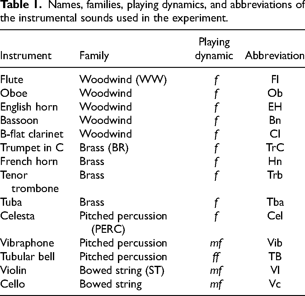
To cover a wide range of instruments allowing for different degrees of blend, 14 different instruments were chosen for the experiment as listed in Table 1, covering all major orchestral families. Sound samples of the 14 instruments were selected from Vienna Symphonic Library (https://vsl.co.at) as stimuli, all playing a sustained D#4 note with ordinary articulation. Samples were downmixed to mono by averaging across the two channels and then trimmed to 2.2 s in duration. A decreasing linear ramp envelope was then applied to the last 200 ms. The generated sound files all had a sampling rate of 44.1 kHz with 16-bit amplitude resolution. To equalize the perceived loudness of the 14 stimuli, 6 volunteers participated in a loudness-matching experiment in which they had to adjust the loudness of all other stimuli to match that of the oboe sample, which functioned as the reference. The medians of adjustment values were applied to the corresponding stimuli except for the celesta sample, for which an additional 2 dB boost was applied because of inadequate loudness boost with the original median value as determined by the authors.
Names, families, playing dynamics, and abbreviations of the instrumental sounds used in the experiment.
The 14 instrumental stimuli were paired with each other, forming 91 pairs in total. It is known that onset synchrony between constituent sounds is an important factor affecting blend (McAdams, 1984). Thus, in the current experiment, the effect of onset asynchrony on blend should be minimized beforehand. To align paired instrument stimuli for creating concurrent blend pairs, seven volunteers participated in an attack synchronization experiment following a design similar to that of Gordon (1987). All combinations of instruments were synchronized by adjusting the relative temporal offset between two isochronous loops of the individual instrument sounds, both having an inter-onset interval of 1 s, until the two instruments sounded as thought they were synchronized and playing on the same beat. The medians of time shift values were applied to corresponding instruments in all pairs. The authors did a final listening check on the synchronized stimuli and made minor adjustments to pairs for which the synchrony was not satisfactory (for time-shift values applied in the experiment, see Table A1 in the Appendix).
Apparatus
The experiment was run with the PsiExp computer environment (Smith, 1995). Sounds stored on a Mac Pro 5 computer running OS 10.6.8 (Apple Computer, Inc., Cupertino, CA) were amplified through a Grace Design m904 monitor (Grace Digital Audio, San Diego, CA) and presented over Dynaudio BM6a loudspeakers (Dynaudio International GmbH, Rosengarten, Germany) arranged at about ±60°, facing the listener at a distance of 1.5 m. Participants were seated in an IAC model 120act-3 double-walled audiometric booth (IAC Acoustics, Bronx, NY). The amplification level of the monitor was chosen in advance by the experimenters after pilot sessions to ensure a comfortable listening level for all stimuli in the experiment and remained fixed for all participants.
Procedure
Participants first read the experimental instructions, were asked what they thought the task was, and were corrected for any misunderstandings. At the very beginning of the experiment, participants were given two examples of instrument pairs that are generally perceived to blend well (violin and cello) and poorly (flute and tubular bell). Well-blended was described as “the sounds fuse together as a single unity in perception when they sound together,” and poorly blended was described as “the sounds are more easily perceived as separate sources when they sound together.” For these two examples, constituent instruments were played one after the other followed by the concurrently sounding pair. Participants then entered a familiarization phase in which 21 instrument pairs (all possible combinations of flute, oboe, trumpet, tuba, violin, celesta, and tubular bell in random order) were played sequentially to give an idea of the possible range of blends they would be rating. 1
The entire experiment was divided into two parts, corresponding to the two blending conditions. As hearing concurrent blend pairs first might prime listeners on the quality of blends and interfere with how they might imagine blends, the condition in which participants had to imagine was presented first. In this part (sequential condition), each instrument sound of the pair was played from both speakers one after the other with a silence of 500 ms in between, and the order of presentation was randomized. Participants were asked to imagine the two instruments being played simultaneously and rate how well the two sounds would blend in the imagined pair by placing a freely movable cursor on a scale with the left end labeled not at all blended (0) and the right end labeled strongly blended (1). Ratings were scaled to 0–1 for analysis. In the second part (concurrent condition), the paired instruments were played simultaneously with the instrument sounds coming out of separate speakers. 2 The assignment of instruments to speakers was randomized. Participants were asked to rate the degree of perceived blend of the sounding pairs using the same scale as in the first part. The order of presentation of instrument pairs was randomized for both parts. Each part was further divided into two blocks, and participants could choose to take a short break between blocks within a part and between the two parts.
Sound Analysis
For the extraction of potential acoustic features related to blend, the Timbre Toolbox (Peeters et al., 2011; revised by Kazazis et al., 2021) was used. Previous studies have pointed out that several temporal and spectral factors contribute significantly to the perception of blend, prominent ones being attack time and spectral centroid (Lembke et al., 2019; Sandell, 1989, 1991; Tardieu & McAdams, 2012), along with various global and local spectral-envelope features (Lembke et al., 2017; Lembke & McAdams, 2015). Given the results of hierarchical cluster analysis on inter-descriptor correlation in Peeters et al. (2011), eight descriptors were chosen (Table 2) and calculated on all single instrument sounds, representing various spectral and temporal features of the stimuli. Attack slope (AttSlope) is a global descriptor computed on the temporal energy envelope of the audio signal that measures the average temporal slope of the envelope during the attack segment. RMS energy (RMSErg) is a time-varying descriptor measuring the root-mean-squared energy of overlapping time frames of the audio signal (window size = 1024 samples, hop size = 512 samples). Spectral centroid (SpecCent), spectral crest (SpecCrest), and spectral variation (SpecVar) are time-varying descriptors addressing the content, shape, and temporal variation of the frequency spectrum of the sound, calculated from the magnitude-squared short-time Fourier transform (STFT) representation of the signal with Hann windows (window size = 2048 samples, hop size = 512 samples). Spectral centroid measures the center of gravity of the spectrum and is usually associated with the brightness of the sound (McAdams, 2013, p. 41). Spectral crest measures the peakiness of the spectrum, which can be used to distinguish between noise-like and tone-like sounds. Spectral variation represents the amount of variation of the spectrum over time. Inharmonicity (InHarm), noisiness, and tristimulus (its three ratio values abbreviated as “Tri1,” “Tri2,” and “Tri3”) are time-varying descriptors addressing the harmonic properties of the sound, calculated from the sinusoidal harmonic partial representation with Blackman windows (window size = 2048 samples, hop size = 512 samples). Inharmonicity measures the deviation of frequencies of partials from pure harmonic frequencies of the fundamental. Noisiness is calculated as the ratio of noise energy (the remainder after harmonic energy has been removed) to total energy in the signal. Tristimulus characterizes the distribution of energies among different partial regions of the spectrum, with the first value (Tri1) measuring the proportion of energy at the fundamental frequency, the second value (Tri2) the proportion of energy of the second to fourth partials, and the third value (Tri3) the proportion of energy of higher partials.
Acoustic descriptors calculated on single instrument sounds, the respective input audio representations used for calculation, and statistics used for summarizing time-varying descriptors. Pairwise associations were used to generate pairwise features.
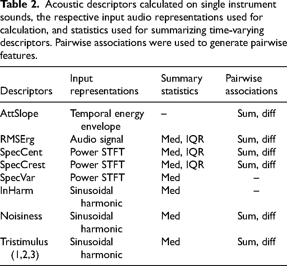
For the time-varying descriptors (all but attack slope), two summary statistics were used to reflect the central tendency (median) and variability (inter-quantile range [IQR]) of the descriptors in a single stimulus. For the current analysis, descriptors showing significant correlations between their own median and IQR values in Peeters et al. (2011) were summarized by median values only. For the rest of the descriptors, both median and IQR were calculated (denoted by suffixes “_Med” and “_IQR” in the abbreviation). In total, there are 13 acoustic descriptor values for each instrument sound. The descriptor extraction process was carried out in Matlab version R2020a (The MathWorks, Inc., Natick, MA).
To model blends with acoustic descriptors, pairwise descriptors were calculated by taking the sum and absolute difference of each single instrument descriptor between the paired instruments, and the generated descriptors are denoted using suffixes “_sum” and “_diff”. Cross-descriptor scatter plots, in which each pair of descriptors was plotted against each other, were used to visually examine if there were continuous mappings between descriptor values. These plots suggest that descriptors of spectral variation and inharmonicity have prominent bimodal distributions in which values cluster unequally at the extremities. As obtaining reliable estimates of the effects of these latter descriptors in a regression model could be problematic, they were not considered in the subsequent analyses. In total, there were 22 pairwise descriptors as potential regressors for modeling blend ratings.
Results
Analyses of data were conducted with R version 4.2.0 (http://www.r-project.org). Results are reported and discussed below.
General Pattern
Median blend ratings were calculated across participants for each instrument pair within each blending condition for each participant group. The correlation between the two blending conditions was calculated with the median ratings for musicians and nonmusicians separately. Overall, both musicians and nonmusicians gave consistent ratings between the two blending conditions, which were highly correlated: For musicians, r(89) = .96, p < .001; for nonmusicians, r(89) = .95, p < .001. This suggests that when two instruments are perceived to blend well when sounding together, they also blend well in imagination.
Inter-rater reliability was calculated for heard blend ratings (i.e., blend ratings obtained from the concurrent condition) and imagined blend ratings (i.e., blend ratings obtained from the sequential condition) separately between all participants. Specifically, ICC2 was chosen as a specific form of intraclass correlation coefficient (ICC) that allows generalization to other raters within the population (Shrout & Fleiss, 1979). Heard blend ratings had a larger ICC (.76) than that of imagined blend ratings (.66), suggesting that participants agreed with each other more when rating heard blends.
ANOVA
A three-way repeated-measures analysis of variance (ANOVA) was subsequently carried out to test the effects of participants’ musical backgrounds (between-subjects factor, musicians vs. nonmusicians), instrument pairs (within-subjects factor, 91 different pairs), blending conditions (within-subjects factor, concurrent vs. sequential), and their interactions on blend ratings. To this end, a linear mixed model was calculated with blend ratings as the dependent variables. Participants were treated as grouping factors across which intercepts were allowed to vary. An ANOVA table with results of F tests and associated p values for the experimental factors and their interactions was extracted from the model using Satterthwaite's method (Satterthwaite, 1946) via the R package “lmerTest” (Kuznetsova et al., 2017). Line plots of mean blend ratings of different instrument pairs (separated according to blending conditions and participants’ musical backgrounds) are supplied in the Appendix to aid the interpretation of the ANOVA results.
For the main effects, the musical background of the participants had no significant effect, F(1, 60) = 1.05, p = .31. The blending condition had a significant main effect on the blend ratings, F(1, 10860) = 474.16, p < .001. Instrument pairs presented in the concurrent condition were generally perceived to blend better than in the sequential condition where participants had to imagine the blends. As expected, the instrument pair had a significant main effect on blend ratings, F(90, 10860) = 352.32, p < .001, reflecting different intrinsic timbral qualities of different instruments that lead to different degrees of blend.
For two-way interaction effects, both the musicians and nonmusicians rated the instrument pairs as more blended on average in the concurrent condition than in the sequential condition. However, there was larger difference of the overall degrees of blend between the two blending conditions for the nonmusicians than for the musicians. Although both groups gave similar overall ratings to the imagined blends, the nonmusicians gave higher overall blend ratings to the heard blends than did the musicians, F(1, 10860) = 18.76, p < .001. Even though the musicians and nonmusicians gave overall parallel ratings across all the instrument pairs, there were still varying degrees of divergence between the two groups for different pairs, F(90, 10860) = 2.11, p < .001, for which no clear explanation emerges. Neither group gave consistently higher or lower ratings than the other group. The interaction effect between instrument pair and blending condition was also significant, F(90, 10860) = 11.07, p < .001. Pairs of two sustained instruments often received higher blend ratings in the concurrent condition than in the sequential condition. On the other hand, pairs of sustained and percussive instruments usually demonstrated the opposite pattern, where the degree of blend was lower in the concurrent condition with overall smaller blend-condition differences (i.e., difference between heard and imagined blend ratings) than for pairs of two sustained instruments. A notable exception concerns pairs involving tubular bell and a sustained instrument, which behaved more similarly to pairs of two sustained instruments.
The three-way interaction between blending condition, instrument pair, and musical background was also significant, F(90, 10860) = 1.44, p = .004. For pairs of two sustained instruments and pairs of tubular bell and other sustained instruments, although the heard blend ratings were usually higher than imagined blend ratings for both groups of participants, the blend-condition difference was frequently smaller for musicians than for nonmusicians. In contrast, for pairs of other percussive instruments and sustained instruments, the blend-condition difference was frequently smaller for the nonmusicians than for the musicians, whereas the imagined blend ratings were often slightly higher than the heard blend ratings for both groups of participants.
Acoustic Modeling
Median blend ratings across all participants in the two blending conditions were treated as outcome variables and modeled separately using a linear regression model with pairwise acoustic descriptors as regressors. Lasso regression was first applied via the R package “glmnet” (Friedman et al., 2010) to select descriptors that made a substantial contribution to predicting blend ratings. 3 Descriptors with non-zero coefficients were subsequently used as regressors in ordinary multiple regression in predicting blend ratings. Table 3 lists the results of multiple regressions for heard and imagined blend ratings separately. Heteroscedasticity-consistent standard errors (SE) calculated with the HC4 estimator (Zeileis, 2004) are reported in Table 3 and used for calculating p values. Lasso regression selected very similar sets of descriptors for the two blending conditions. The only unique descriptors belonging to either the heard or imagined blends are the differences of medians for tristimulus 1 and tristimulus 3, respectively.
Model estimates for heard and imagined blend ratings (

Note. *: p ≤ .05, **: p ≤ .01, ***: p ≤ .001
Multidimensional Scaling
Multidimensional scaling (MDS) is a useful tool for visualizing proximity data and uncovering latent dimensions of judgment (Borg et al., 2018). Blend ratings can be conceived as a specific type of proximity data, with higher blend ratings suggesting a kind of affinity between the associated instruments, as was done in studies by Sandell (1989, 1991). The derived multidimensional space, therefore, can be understood as a “blend space” in which closely spaced instruments tend to blend better than instruments that are farther apart. For the current study, computing such spaces offers a straightforward way to compare how instruments are perceived to blend in the two experimental conditions. For each condition, each participant's blend ratings were subtracted from 1 to generate pairwise “dissimilarity” data. These “dissimilarity” data were modeled with metric INDSCAL (Carroll & Chang, 1970) using the R package “smacof” (de Leeuw & Mair, 2009). INDSCAL uses all individual participants’ data by allowing individuals to have different weights on each dimension of the underlying group configuration, generating a configuration that considers individual variation. Following across-subjects cross-validation procedures using jackknifing and model evaluation procedures based on the Aikake Information Criterion (AIC) described by Elliott et al. (2013), two-dimensional INDSCAL was found to give the best solution-balancing model fit and parsimony for both heard and imagined blend ratings. The overall Stress values of the INDSCAL solutions for heard and imagined blend ratings were .26 and .27, respectively.
The blend space for heard blends was transformed with Procrustean transformations to match that for imagined blends to allow the structures of the two spaces to be more easily compared. To show potentially meaningful acoustic dimensions underlying the blend spaces, the acoustic descriptors calculated on single instrument sounds (see Table 2) were projected onto the blend spaces by regressing each descriptor on the instruments’ coordinates along the two dimensions:

INDSCAL configurations of heard and imagined blend ratings, along with projections of acoustic descriptors having individual R2 values that are significant at the .05 level.
For both blend spaces, a prominent feature is that instruments are separated into two groups of percussive instruments and sustained instruments on the first dimension, which can be primarily attributed to the attack slope. The space occupied by sustained instruments seems to be more compact in the concurrent condition. This corresponds to the ANOVA results discussed earlier that pairs of sustained instruments tend to blend better when heard than in imagination. For heard blends, AttSlope, Tri1_Med, Tri2_Med, and Noisiness_Med appear to be significant descriptors in both the regression modeling of blend ratings presented in the previous section and projections of acoustic descriptors in the blend space. For imagined blends, the shared descriptors between the regression model and projections in the blend space are AttSlope, Tri2_Med, Tri3_Med, and Noisiness_Med. Although both regression models discussed in the previous section and projections of acoustic features in MDS spaces aim to find acoustic correlates of blend ratings, they model and abstract blend information in different ways that give overlapping but still different results. Given that the regression models only use median ratings across participants, whereas INDSCAL models consider individual variation in the raw ratings explicitly, a greater emphasis is placed on the results of the acoustic projections in the MDS spaces for the rest of the article.
Comparing the two blend spaces, SpecCent_Med and Tri3_Med have significant correlations with the spatial positions of the instruments in the imagined blend space but not in the heard blend space. Both descriptors appear to be meaningful acoustic dimensions explaining the second dimension of the imagined blend space. Other than these two descriptors, the two blend spaces share the same significant acoustic projections, the directions of which are nevertheless different in the two blend spaces.
Discussion
Given that previous studies have shown the kinship of neural activities associated with the timbral imagery of an instrument sound and that of hearing it (Halpern et al., 2004), it seems logical that listeners would give overall coherent ratings of heard and imagined blends. Meanwhile, it is also plausible that features of instrument sounds will be extracted differently by listeners when imagining blends compared with when evaluating heard blends because of limited attentional resources involved in imagining blends, which might lead to different degrees of divergence between the two types of blends for different instrument combinations. The overall coherence between heard and imagined blends is confirmed by the strong correlation between blend ratings in the two experimental conditions. Most notably, the big picture holds true for both types of blends: Pairs containing one percussive and one sustained instrument blend universally worse than all the other pairs, as previously found by Tardieu and McAdams (2012) and Lembke et al. (2019).
Despite the overall parallel, various degrees of difference between the two types of blends are still observed. Qualitatively, many participants reported verbally after the experiment that many pairs blended much better when they heard them being played compared to what they previously imagined, which is in line with the significant main effect of blending condition on blend ratings. This global pattern holds true when inspecting the data from musicians and nonmusicians separately. It seems plausible that despite people's ability to imagine two instruments blending, in the case of the current experiment, the imagination of blends seems to be on average more “conservative” than the hearing of actual blends in terms of the degree of blend. A possible explanation of this, as confirmed by some participants’ feedback, could be attributable to the constructive nature of mentally blending two existing instruments: Operating on the mental images of two distinct instruments assumes a priori the “twoness” of the composite sound.
The exact nature of the differences between heard and imagined blends is largely dependent on the specific instrument pairs in question. Blends of two sustained instruments were generally underestimated in imagination, and blends of one percussive and one sustained instrument were generally similar or slightly overestimated in imagination. It seems plausible that for instruments with sharp contrasts in their attack behaviors, their blends were relatively easy to conceive in imagination and the rating was driven by the apparent difference in attack as a signifier of nonblend. Thus, they were in general given low ratings, which were not too different from the perception of hearing the blends, apart from the tubular bell. For instruments without apparent attack contrasts, blends were harder to conceive and evaluate in imagination, possibly because of the generic difficulty of superimposing two instruments’ images in imagination and the intrinsic “twoness” of the imagination task. The difficulty of imagining blends could also be implicitly inferred from the smaller ICC for the imagined blend ratings compared to heard blend ratings, as participants overall had more diverging imagined blend ratings for the same instrument pair.
Previous studies on retention of timbre in working memory have suggested that deterioration of memory can happen with reduced attentional resources, upon which maintenance of timbre through attentional refreshing relies (Siedenburg & McAdams, 2017b). It is possible that the action of retaining two instruments in memory and subsequently superimposing them internally requires a certain level of attentional resource (Soemer & Saito, 2015), which might detract from the accuracy of the blend's representation. Consequently, participants might be less confident to rate their imagined blends as either very well blended or badly blended. This is partially reflected in the distribution of raw blend ratings from all participants on all instrument pairs: whereas heard blend ratings are more populated near both ends of the rating scale, imagined blend ratings are relatively more spread across the entire scale. Another possible explanation of heard blend ratings being more polarized than imagined blend ratings is linked to the ordering of the experimental conditions. The imagination task with its associated difficulty in the first part likely conditioned and heightened participants’ expectation of what good or bad blends sound like. The exposure to heard blends in the second part thus confronted participants with fresh stimuli that were easily accessible to evaluation. This augmented state of realization of aspects of blends (e.g., “I didn't expect this pair to blend that well/badly until I heard it,” which showed up in feedback from participants) possibly encouraged participants to rate with more confidence, thus leading to more polarized ratings observed in the concurrent condition (i.e., blends tend to be either rather good or rather bad when heard).
The pairing of the tubular bell with sustained instruments stands out from that of other percussive instruments as all its pairs were perceived to blend somewhat better when heard than when imagined (in contrast to the other pairs of percussive and sustained instruments). The inharmonic sound along with the perceived indefiniteness of pitch of the tubular bell plausibly suggests to participants its inability to blend with other instruments, as all the other instruments have more harmonic sounds with clearly defined pitches. 4 When blends were heard, however, the sound of the tubular bell was able to blend with others to a better degree, possibly due to spectral masking and complex interactions between frequencies of the paired sounds. On the one hand, this again points to the fact that blends in imagination are probably not able to preserve and account for the actual acoustic interactions happening within heard blends. On the other hand, it suggests that the evaluation of blends in imagination might be biased by simply evaluating the similarity between constituent instruments, as the immediacy of the tubular bell's uniqueness possibly explains its low blend ratings when paired with other instruments in imagination. This latter point will be discussed in more detail in Experiment 2.
The significant three-way interaction between musical background, instrument pair, and blending condition suggests that musical background may play a role in how blends are imagined vs. heard for different instrument pairs. In the current experiment, the underestimation of blends of two sustained instruments as well as pairs including tubular bell is more prominent in nonmusicians than in musicians, where musicians’ blend ratings are more similar between the two blending conditions. This pattern is, however, slightly reversed for pairs of other percussive instruments and sustained instruments. A possible explanation is that spectral cues (e.g., masking between instruments) are relatively more available to musicians when imagining blends compared to nonmusicans. Because of exposure to instrumental practice where both inner hearing and “external” hearing are frequently involved, musicians may have a higher sensitivity to differences between instrumental timbres. As a result, for pairs of instruments without sharp attack contrast, the imagined blends from musicians more frequently matched heard results better than in the nonmusicians’ case. For nonmusicians, the attack contrast between blending instruments is a much more available cue than are spectral cues for judging blend in imagination. Thus, for some pairs with a significant presence of attack contrast compared to other spectral cues that on the contrary suggests the potential for blending, 5 non-musicians seemed to discount the plausible promoting factor of spectral similarity more and gave more matching heard and imagined ratings than musicians did. Musicians, on the other hand, seemed to account for different aspects of sounds more thoroughly when imagining blend, even though in the end the attack contrast turned out to be a much stronger cue for non-blend when heard.
Acoustic modeling of blend ratings in the concurrent and sequential conditions suggests a similar set of features that may explain the ratings. The model for heard blend ratings shares a few similar acoustic descriptors with the one obtained in Sandell (1991) for unison blends, including AttSlope_diff and a few other tristimulus features. In line with Sandell's model, the negative coefficient of AttSlope_diff suggests that a large difference between attack behaviors leads to worse blend. The prominence of tristimulus-related features found in models of both blending conditions possibly suggests a substantial role of acoustic features related to contrasts of spectral envelopes between the blending sounds, which have already been discussed by Lembke and McAdams (2015) and Reuter (1997) in terms of sounding blends. In the current experiment, both types of blend ratings decreased when the sounds of blending instruments had large differences in one or more tristimulus coefficients. Notably, imagined blends were more strongly affected by tristimulus 3, which describes the richness of high partials, than heard blends.
Some of the results in acoustic modeling of blend ratings are also reflected in MDS modeling, which considers variations between individual participants. When examining the projections of acoustic descriptors in blend spaces, certain significant descriptors (e.g., contrasts between attacks, noisiness, second tristimulus value, etc.) are shared by both spaces, suggesting some invariant aspects when evaluating heard and imagined blends. Notably, the projections of Tri3_Med and SpecCent_Med are not significant in the heard blend space but emerge as important in the imagined blend space. The emergence of tristimulus 3 in imagined blends is also observed in the regression modeling of blend ratings discussed above. These findings suggest that when participants imagine blends, a primary focus is on the brightness and richness of the high partials of the two sounds. If the blending sounds are very different on these acoustic aspects, they are less likely to blend well in imagination because of their uniqueness. On the other hand, these two features seem to be less relevant for the evaluation of heard blends. This could be attributed to spectral masking and the interaction between frequencies that occurs in perceived blends, which were not faithfully accounted for in imagination but effectively led to higher blend ratings with physically sounding stimuli. Another possible explanation of the reduced relevance of these spectral features has to do with the more polarized blend ratings observed for heard blends. This polarized pattern accentuates the effect of attack contrast in the perception of heard blends, and at the same time, this effect might have masked the less prominent effect of some spectral features, which also led to their poor fit in the models.
On a global level, the absence of significant projections of spectral centroid and tristimulus 3 in the heard blend space (which otherwise have a similar set of underlying acoustic projections) plausibly collapses the instruments into a smaller space compared to the imagined blend space. This collapse happens as the variation between instruments on these two spectral features does not contribute significantly to the spatial variation of sounds in the blend space (thus resulting in better blends in general). Some of the individual differences between instruments that are deemed to be prohibitive to blends in imagination become less influential for good blends with heard sounds. In the end, one could also surmise that evaluating blends in imagination resorts to judging the dissimilarity between blending instruments, instead of a purely mental recreation of the two instruments sounding together. Based on these comparisons and some participants’ feedback, it seems that there is an underlying analytical or comparative inclination when imagining and evaluating blends: Certain differences and contrasts between two sounds are intuitively interpreted as signifiers of nonblend, without necessarily undergoing the supposed mental process of superimposing the two timbres. To provide more concrete evidence of this hypothesis, a follow-up experiment using the same stimuli with participants rating the perceived dissimilarity between instruments was thus conducted.
Experiment 2
Method
Participants
A different group of 48 participants from Schulich School of Music at McGill University and the general Montréal community participated in the experiment. Two participants’ data were not included in subsequent data analyses as they did not pass the quality check (see the Procedure section below). Thus, 46 participants were included in the analyses (male = 16, female = 28, non-binary = 2) with an average age of 25 years (SD = 8.4). Unlike Experiment 1, the current experiment did not differentiate participants based on their musical backgrounds. A wide range of musical backgrounds were thus present in the participants recruited, with an average of 9 years of musical training and practice (SD = 8.7). Before the experiment, participants passed the same pure-tone audiometric test as described in Experiment 1. They were paid for their participation. The experiment was certified for ethical compliance by McGill University's Research Ethics Board II. All participants signed written consent forms before the experiment.
Stimuli
The same individual stimuli as Experiment 1 were used. The 14 instrumental sounds were paired with each other sequentially and additionally with themselves (i.e., pairs of identical sounds), forming 105 pairs in total.
Procedure
The same apparatus as Experiment 1 was used. After reading the instructions, participants entered a familiarization phase in which all 14 instrumental sounds were played one by one in random order to give participants an idea of the scope of sounds to be compared. In the main experiment, paired sounds were played one after the other (with a gap of 0.5 s in between), and the order of presentation within the pair was randomized. Participants were asked to rate how dissimilar the two sounds were by placing a freely movable cursor on a scale with the left end labeled identical (0) (i.e., the same sound presented twice) and the right end labeled very dissimilar (1). Ratings were scaled to 0–1 for analysis. The order of presentation of instrument pairs was randomized. Before entering the main experiment, participants additionally completed practice trials in which they rated 10 randomly selected instrument pairs using the same interface as in the main experiment. Data from the practice trial were not used. The main experiment was divided into two blocks, and participants could choose to take a short break between blocks. A preliminary check on the ratings given by participants for the identical instrument pairs showed that two participants gave abnormally high ratings to some of these pairs, for which the ratings should be theoretically very close to 0. 6 For reasons of quality control, these two participants were excluded from the subsequent data analyses given that their data seemed to be less reliable.
Results
General Pattern
Correlation analyses were conducted between median dissimilarity ratings and median blend ratings from Experiment 1 (separately for concurrent and sequential conditions) across all participants for all 91 different instrument pairs to show the overall congruence between instrument dissimilarity and blend ratings. The two correlation coefficients calculated individually for heard and imagined blend ratings were compared using the R package “cocor” (Diedenhofen & Musch, 2015) to test if there was a statistically significant difference between the magnitudes of the two correlations.
Both types of blend ratings show strong negative correlations with dissimilarity ratings: For heard blends, r(89) = −.93, p < .001; for imagined blends, r(89) = −.99, p < .001. Therefore, instruments blend worse if they are perceived to be very dissimilar for both types of blends. Numerically, imagined blend ratings show a larger magnitude of correlation with dissimilarity ratings than heard blend ratings do. Several methods exist to compare dependent correlation coefficients (i.e., correlation between data collected on the same samples) and examine the statistical significance of their difference. The R package “cocor” implements 10 different methods ranging chronologically from Pearson and Filon's z (1898) to Zou's (2007) confidence interval to compare the two correlation coefficients between the two types of blend ratings and dissimilarity ratings. All 10 methods rejected at the .05 alpha level the null hypothesis that these two correlation coefficients are the same, meaning that imagined blend ratings do show a statistically larger negative correlation with instrument dissimilarity ratings than heard blend ratings do.
ICC was calculated for the dissimilarity ratings as was done for the blend ratings in Experiment 1. The dissimilarity ratings in Experiment 2 had about the same ICC (.66) as that of the imagined blend ratings.
Principal Component Analysis
Additional analyses were conducted to examine the relationships between instrument dissimilarity, heard blend, and imagined blend ratings while considering variation across individual participants. Principal component analysis (PCA) was conducted by treating the 91 different instrument pairs as individuals and the 3 types of perceptual ratings given by individual participants as “feature variables” (dissimilarity [N = 46] and two blends [N = 62 in each case]), which leads to 170 variables. Calculating principal components of these feature variables will uncover whether there are general relationships among the three sets of ratings above and beyond individual variation among participants. PCA was conducted using the R package “FactoMineR” (Lê et al., 2008).
The first two principal components (PCs) explained around 77% of the total variance in the data. A correlation plot of feature variables (i.e., individual participants’ ratings on the 91 pairs of instruments) on the first two PCs is shown in Figure 2, in which the coordinates of a feature on the two PCs correspond to their correlation coefficients. The plot shows that feature variables cluster together according to whether they are dissimilarity, heard blend, or imagined blend ratings. This suggests that on these two PCs, the three types of perceptual ratings can be systematically differentiated, and within each of the three types of ratings there is inner consistency across participants. Plotting variables on other PCs with eigenvalues larger than 1 shows no clear differentiation of the three sets of ratings on the other PCs, which could be attributed to individual variances between participants, and they are not further considered here. The 91 instrument pairs, which were treated here as individuals in the PCA, were also plotted according to their component scores on the two PCs (see Figure 3).
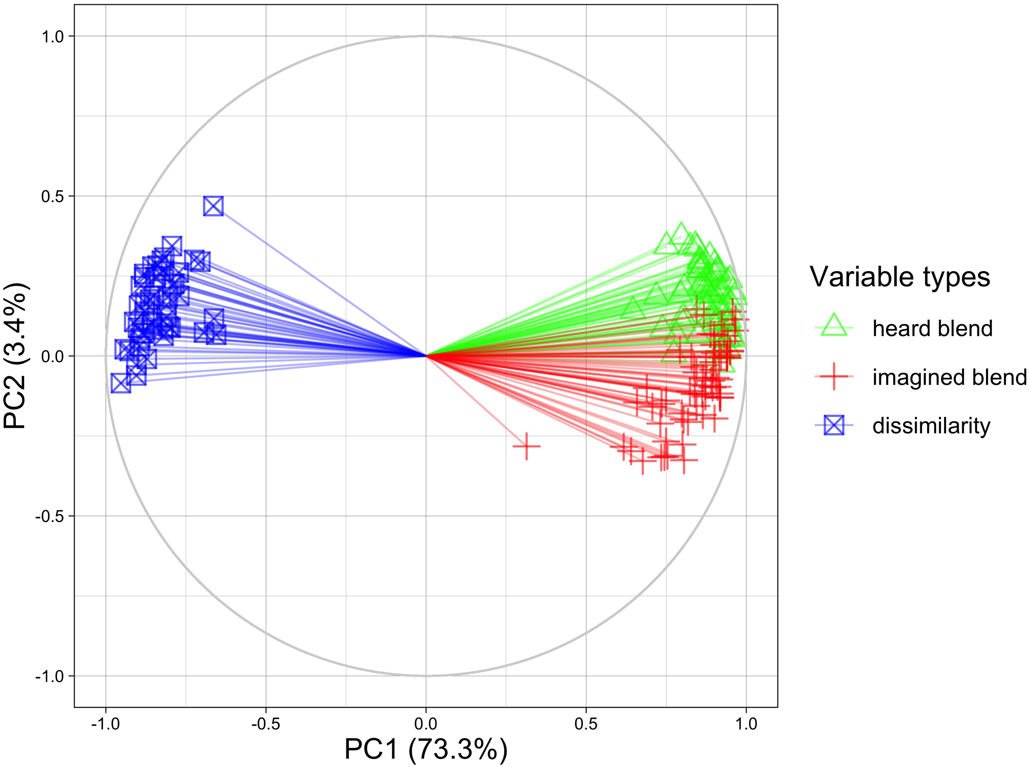
Correlation plot of feature variables (individual participants
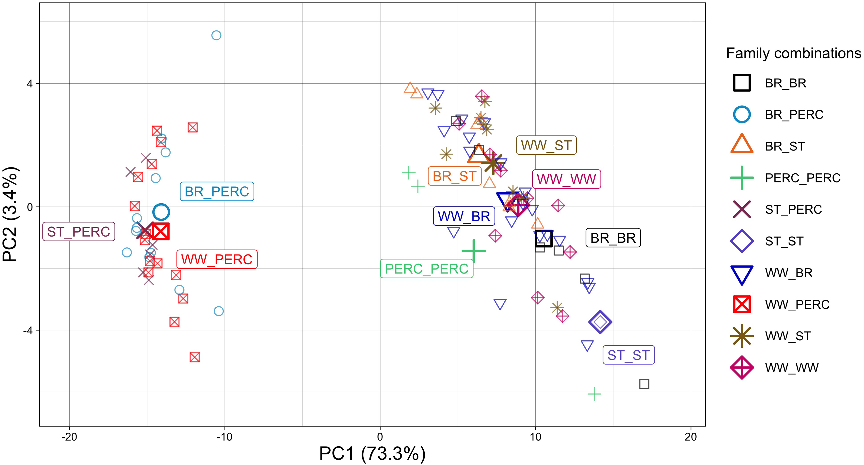
Instrument pairs
The first PC in Figure 2 clearly separates the two types of blend ratings from the dissimilarity ratings as they point in opposite directions in the correlation plot, meaning they are negatively correlated. In Figure 3 with instrument pairs, the first PC separates pairs with both percussive and sustained instruments from pairs with similar attack behaviors. As discussed in Experiment 1, pairs of mixed attack behaviors always received the lowest blend ratings regardless of being heard or imagined. It can be inferred that the first PC describes different degrees of generic blending qualities of instrument pairs, where higher scores mean better blends. As imagined blends and heard blends are highly correlated, these two both contribute in the same manner to the first PC, combining into a single measure of instrument pairs’ ability to blend. It is also expected that dissimilarity ratings contribute oppositely to this PC given its negative correlation with both blend ratings. The singularly large eigenvalue of this PC (124.6) compared to the other PCs (all below 10) indicates that variance in different instrument pairs’ intrinsic blend qualities is the predominant source of variance in the data.
The separation of clusters of heard blend ratings and imagined blend ratings on the second PC in Figure 2 suggests that this PC is related to the contrast between the two types of blend ratings and represents the second largest variance in the data, albeit much smaller (3.4% of the total variance). This can be quantitatively tested by correlating the difference between median heard blend ratings and median imagined blend ratings across all participants and the component score on the second PC for all instrument pairs. The correlation is highly significant, r(89) = .81, p < .001. Thus, the second PC is interpreted as describing the degree of difference between heard and imagined blend ratings of instrument pairs (not absolute difference), where higher scores mean instrument pairs blend much better when heard than when imagined. The eigenvalue of the second PC is much smaller than that of the first PC but still larger than 1, meaning that the variance of blend-condition differences among instrument pairs is still a significant source of variance in the data.
Overall, one can see in Figure 2 that dissimilarity ratings show a larger negative correlation with imagined blend ratings as their clusters occupy opposite quadrants in the correlation circle and point in nearly opposite directions. Indeed, if dissimilarity was transformed into similarity, the projections would overlap with those of imagined blend.
Multidimensional Scaling
Parallel to the MDS analyses done for blend ratings in Experiment 1, dissimilarity ratings in the current experiment were also submitted to the 2D INDSCAL model. The overall Stress value for the INDSCAL solution was .27. The generated dissimilarity space was matched to the imagined blend space described in Experiment 1 with a Procrustean transformation. Acoustic descriptors were projected onto the transformed dissimilarity space as was done with the heard and imagined blend spaces in Experiment 1. Eventually, the same set of significant projections as in the imagined blend space was found for the dissimilarity space, with almost identical directions of projections. The transformed dissimilarity space is plotted on top of the heard and imagined blend spaces derived from Experiment 1 in Figure 4. Note that the two blend spaces were aligned and scaled with a Procrustean transformation in Experiment 1.

Dissimilarity space plotted on top of the heard blend space (“blend_concurrent”) and imagined blend space (“blend_sequential”). The same instrument is connected by an arrow originating from the blend spaces.
Comparing the three INDSCAL solutions visually, it is easy to see the greater similarity between configurations of dissimilarity and imagined blend ratings. The similarity between the two blend spaces and the dissimilarity space was quantified using the alienation coefficient (Mair et al., 2022), where a higher coefficient signifies a larger configuration difference. Benchmarked against a large number of comparable random configurations (N = 1,000) from which an empirical null distribution of alienation coefficient differences was calculated, the alienation coefficient between the imagined blend space and the dissimilarity space (.11) was significantly smaller (p = .004) than that between the heard blend space and the dissimilarity space (.32).
Discussion
The impetus behind Experiment 2 was to test the hypothesis posed when discussing the results from Experiment 1 that evaluating imagined blends is strongly informed by judging dissimilarity of the blending instruments rather than by an ideal mental re-creation of a blended timbral image. Correlation analyses show that, although both imagined and heard blend ratings correlate significantly and negatively with dissimilarity ratings, dissimilarity ratings do correlate statistically more strongly with imagined blend ratings than with heard blend ratings, which provides support for the hypothesis.
A previous study by Kendall and Carterette (1993) had already investigated the relationship between the perceived degree of heard blend and instrument dissimilarity for wind instruments. They found that the degree of blend could be rather well predicted by the distance between the constituent instruments in a 2D perceptual similarity space generated by a musicologist who positioned instruments along two predetermined timbral semantic axes based on mental imagery of timbre. The kinship between dissimilarity space and blend space is indeed observed in the current experiment with direct measurement of perceived dissimilarity. However, when one compares heard blends and imagined blends, the blend space of imagined blend shows a stronger structural similarity with instrument dissimilarity space. This result again echoes the correlation analysis that instrument dissimilarity ratings correlated significantly more highly with imagined blend ratings than with heard blend ratings. Additionally, the very similar ICCs of dissimilarity ratings and imagined blend ratings (in comparison to heard blend ratings) also suggests a kinship between the tasks of rating instrument dissimilarity and rating imagined blends in the current experiments.
Additionally, when comparing the dissimilarity space and the heard blend space, one notices a clear dilation of instruments when moving from the latter to the former (as shown by the arrows in Figure 4). The same is true when comparing imagined and heard blend spaces (see Figure 1). One may also notice that this dilation of instrument space is more prominent along the second dimension, which relates prominently to spectral centroid and tristimulus 3 of the sounds in the dissimilarity space. A rough quantitative examination of this observation can be achieved by comparing the standard deviation of instruments’ coordinates on each dimension (as a measure of spread) between different spaces (Table 4). Results confirm the qualitative observation that the instruments are more spread out on the second dimension when moving from the heard blend space to the dissimilarity space. As instruments in the heard blend space are not significantly distinguished in terms of spectral centroid and tristimulus 3 (neither descriptor has a significant projection in the heard blend space), the dilation of instruments on the second dimension in the dissimilarity space suggests increased relevance of the stimuli's spectral centroid and tristimulus 3 when rating their dissimilarity compared to rating their blends when heard. Echoing the observation made when discussing Experiment 1, this finding suggests that sounds judged to be dissimilar in terms of their brightness and richness of high partials, which were also thought to be unable to blend well in imagination, were often able to blend relatively better when heard than expected.
Differences of standard deviation of instruments’ coordinates on each dimension between INDSCAL spaces.
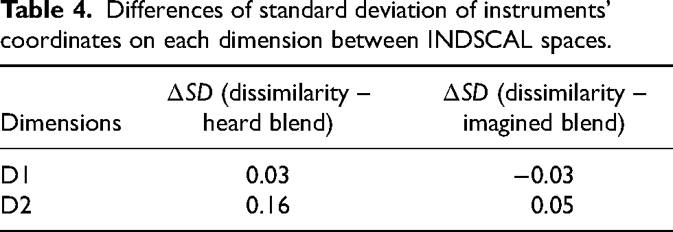
A much subtler dilation of instrument space can also be observed when moving from the imagined blend space to the dissimilarity space. As in the case of the heard blend space, the dilation happens more prominently along the second dimension (especially for Tba, Bn, Cl, Hn, Ob, Vl, and Vc), which is also supported by the results in Table 4. This could suggest that when judging imagined blends, the dissimilarity in brightness and harmonic energy in the high-frequency range between blending sounds still played a role but was also attenuated by participants compared to when they were asked to judge the dissimilarity. This likely suggests the presence of actual mental re-creation of blended timbral composites that mitigates the negative effect of differences between blending sounds rather than simply a process of judging dissimilarity.
More subtle relationships among instrument dissimilarity, heard blend, and imagined blend ratings were explored with PCA by treating individual participants’ ratings as feature variables. As visualized in the correlation plot of individual participants’ ratings (Figure 2), the first two PCs separated the three types of perceptual ratings into individual clusters, and overall dissimilarity ratings show a larger negative correlation with imagined blend ratings than with heard blend ratings. The first two PCs encoded the global variance related to instrument pairs’ generic ability to blend according to how dissimilar they are (the first PC) and blend-condition differences (the second PC). Looking at how the three types of ratings relate to the second PC, it is easy to observe that the difference between heard and imagined blend ratings, which explains the second PC as discussed in the section on PCA results, is to some extent positively associated with the degree of dissimilarity between the blending instruments (note in Figure 2 that the clusters of dissimilarity vectors have a projection in the positive direction on the second PC). This means that the perceived dissimilarity, which prominently relates to worse blends in imagination, is not as adverse for heard blends. In other words, the imagined blend of two instruments that are perceived to be more dissimilar can be more easily “challenged” when the blend is heard, which is often more blended than in imagination. Note that this positive association between dissimilarity and blend-condition difference is limited to discussing pairs with similar attack behaviors and should not be extended across the entire set of instrument pairs because pairs with large attack contrasts always receive much higher dissimilarity ratings than those with similar attack behaviors but do not necessarily have larger blend-condition differences.
General Discussion
The inclusion of instrument dissimilarity data from Experiment 2 substantiates the comparison of heard and imagined blends in terms of a possible underlying mechanism for evaluating imagined blends. It is thus worth revisiting some of the results from the two experiments especially in light of the addition of dissimilarity data.
A notable feature in the score plot of instrument pairs on the first two PCs from Experiment 2 (Figure 3) that has not been discussed is the different orientations of the two groups of instrument pairs separated according to homogeneous or heterogeneous attack behaviors. For pairs with homogeneous attack behaviors (clustered on the right side in Figure 3), blend-condition difference and instrument dissimilarity (PC 2) have an overall negative relationship with the intrinsic blend qualities of instrument pairs (PC 1). More specifically, pairs that clearly blend well when either heard or imagined are usually highly similar instruments. Imagined and heard blend ratings of them are very close together, with the former sometimes being slightly higher. On the other hand, pairs that have less obvious blending qualities where the degree of blend is usually in the middle range and therefore somewhat ambiguous are usually those containing more dissimilar instruments. They often received diverging blend ratings, which were usually higher when those pairs are heard as compared to being imagined. This relationship is observed when blending instruments have very similar attack behaviors where listeners would primarily rely on spectral information to judge the quality of the blend. However, for pairs with contrasting attack profiles (clustered on the left side in Figure 3), listeners’ attention might focus on this more dominant distinction between instruments when evaluating blends at the cost of perceptual resolution for the relatively less pronounced spectral differences (Lembke et al., 2019). Translating this to Figure 3, these pairs are therefore squeezed into a narrow range of the poor-blend zone on the far left, and there is no visible association between their intrinsic blend qualities and blend-condition differences. The variance along the second PC for these heterogeneous pairs plausibly captures the varying “residual” dissimilarity in the spectral domain between blending instruments when excluding their predominant attack differences. This portion of dissimilarity is of relatively smaller perceptual prominence and pertains to the differing blend-condition differences observed among these heterogeneous pairs.
A few more observations can be made regarding the categorization of instrument pairs according to instrument family combinations, by which the individual points in Figure 3 are shaped. As the numbers of instruments are not balanced among instrument families, the following observations are only qualitative but nevertheless worth discussing. Focusing on pairs with homogeneous attack behaviors, one notices that pairs of instruments from the same family in general blend relatively well and have smaller blend-condition differences (i.e., their blends tend to be more consistent when imagined and heard). In contrast, cross-family combinations do not blend as well, but it happens more often that these combinations have the potential to blend better than people would imagine. The combinations of woodwind and brass instruments cover the greatest range of the blend palette, containing many pairs that clearly blend well or blend well rather “unexpectedly” when heard. Stringed instruments are usually perceived to be quite different from wind instruments, but they are able to create rather good blends with different woodwind and brass instruments when heard.
When looking at INDSCAL configurations generated for dissimilarity and blend ratings, it is especially interesting to note the migration of the French horn and the oboe between spaces, as they move from the periphery in the dissimilarity space and imagined blend space to the center of instrument clusters in the heard blend space. This suggests their ability to blend relatively well with many different instruments. Specifically, the ability of the French horn to blend well with other instruments and function as a bridge instrument drawing different groups of instruments into a blend has been well discussed in the orchestration literature (Piston, 1955; Riddle, 1985). Their affinity to blend relatively well with other instruments in the concurrent condition could be first explained in terms of the conditioning effect of having to imagine blends first in the experiment, where heard blend ratings were augmented in relation to imagined blend ratings, as discussed in Experiment 1. Additionally, one may also consider the blend-promoting factor of spectral masking present in the sounding composites, where the bright and nasal timbre of the oboe can mask other instruments, whereas the French horn is susceptible to being assimilated into other instruments’ timbres. These acoustic factors remain subordinate to dissimilarity between instruments when judging imagined blends, thus the two instruments do not appear to be good blenders in imagination.
The hypothesis that Experiment 2 examines implies a causal relationship between two mental processes, where dissimilarity perceived between instruments leads to poorer imagined blends. So far, this causality has been assumed throughout discussion of the results. Although there is no direct testing of the causality, we speculate that at least part of the causality could be implicitly satisfied according to the experimental design. The sequential presentation of sounds used for inducing blend imagination in the experiment could have somewhat facilitated the mental process of comparing sounds, whether it is explicitly practiced by participants to aid their rating of imagined blends prior to the latter process or unintentionally/implicitly resorted to while evaluating the imagined blending timbral image. Nevertheless, we recognize that a theoretically sound examination of the nature of and relationship between blend imagination and dissimilarity ratings (i.e., whether dissimilarity ratings happen in concert with or even in place of the hypothesized sensory re-creation of blending timbres) would be more viable with the help of neuroscientific methods.
Conclusion
The current research assessed how instrumental blends are imagined from the presentation of individual instrumental sounds in succession in comparison with the perception of blend of physically sounding dyads. The results show that macroscopically, imagined blends are largely consistent with heard blends. On a microscopic level, how well the imagined images of blends correspond to the heard blends is contingent on the complex interaction between the specific instruments involved and the participants’ musical backgrounds. For pairs involving both percussive and sustained instruments, their blends can be readily conceived and evaluated in imagination relying on the contrasting attack profiles of the instruments, therefore most closely matching the perception of their heard blends. Without this cue, blends can be harder to properly conceive in imagination, and the degree of blend is usually underestimated in imagination. Additionally, this underestimation is overall more prominent in nonmusicians, whereas musicians’ blend ratings are more similar between the two blending conditions.
Regression modeling of blend ratings and projection of acoustic descriptors in the blend spaces obtained with multidimensional scaling suggest that, although both types of blend are affected by a few common acoustic descriptors (e.g., contrasts between attack behaviors, noisiness, second tristimulus value, etc.), the evaluation of imagined blend is more sensitive to differences in brightness and richness of high partials between the paired sounds, represented by the spectral centroid and tristimulus 3. Sounds that are different on these acoustic features tend to receive lower blend ratings in imagination. For physically sounding dyads, these acoustic differences are likely mitigated due to masking and interference between the spectra, which allow better blends to happen. It seems plausible that it is difficult for the mental faculty to fully account for the complex acoustic interactions occurring between sounds that may affect the actual blends. A “comparative” strategy, by which sounds are analyzed according to their differences and uniqueness, thus plausibly underlies the evaluation of imagined blends, rather than an authentic mental image of the blend as a timbral composite. This kinship between evaluating imagined blend and judging instrument dissimilarity is again supported by the results from Experiment 2.
Future directions following the current study can be addressed in three aspects. The ordering of the two experimental conditions in the current experiment may have had an effect on how participants evaluate blends. While presenting the sequential condition first can help bypass the priming effect of presenting concurrent blends to participants first, it probably brought in other biases where heard blend ratings were potentially augmented and polarized. Randomizing the order of presentation as a comparative follow-up experiment would allow us to evaluate whether such biases exist. Meanwhile, it seems logical that a more musically meaningful examination of the properties of timbral imagination should allow for a larger musical context. Composers rarely focus on the blends of two static single notes. Phrasal, melodic, or even textural organizations thus may serve as meaningful musical contexts for future explorations on timbral imagination, allowing a more organic and ecologically valid investigation of other possible musical attributes that affect blends in imagination. Finally, the yet-unanswered question of what happens when people actively imagine blends calls for cognitive neuroscientific approaches to elucidate the underlying mechanisms. Some participants reported after the experiment that they did not always or were not always sure that they followed the instruction of imagining the two sounds playing simultaneously (as it was not always easy) but rather switched to other methods momentarily, such as holding the first note in memory and superimposing its image onto the second note being played where evaluations were made on this “half-imagined” blend. Other methods reported include simply judging the similarity between instruments as a shortcut to rate how they blend in imagination. Methods such as functional magnetic resonance imaging (fMRI), as adopted in Halpern et al. (2004), might shed light on how comparable imagining blends is with hearing blends or simply comparing two sounds on a neurological level.
Supplemental Material
sj-zip-1-mns-10.1177_20592043241246751 - Supplemental material for Comparison of Heard and Imagined Blends of Instrumental Dyads
Supplemental material, sj-zip-1-mns-10.1177_20592043241246751 for Comparison of Heard and Imagined Blends of Instrumental Dyads by Linglan Zhu and Stephen McAdams in Music & Science
Footnotes
Acknowledgements
The authors would like to thank Bennett K. Smith for programming the experiment interface for both experiments and Marcel Montrey for offering input on the statistical analyses.
Action Editor
Charalampos Saitis, Queen Mary University of London, School of Electronic Engineering and Computer Science.
Peer Review
Isabella Czedik-Eysenberg, University of Vienna, Department of Musicology.
Sven-Amin Lembke, Anglia Ruskin University, Cambridge School of Creative Industries.
Contributorship
LZ researched literature and conceived the study. LZ and SMc were involved in study design, gaining ethical approval, participant recruitment, and data analysis and interpretation. LZ wrote the first draft of the manuscript. LZ and SMc reviewed and edited and approved the final version of the manuscript.
Experiment 1 reported in this article was conceived in the context of the Master's thesis research of the first author (Zhu, 2022). Part of the reported results in this article were presented and collected in the proceedings of the following conferences: the 3rd International Conference on Timbre (Timbre 2023), Thessaloniki, Greece; the 17th International Conference on Music Perception and Cognition (ICMPC), Tokyo, Japan.
Declaration of Conflicting Interests
The authors declared no potential conflicts of interest with respect to the research, authorship, and/or publication of this article.
Ethical Approval
This study was approved for ethical compliance by McGill University's Research Ethics Board II. REB File No. 162-0817 / September 10, 2021.
Funding
This project was funded by a Canadian Natural Sciences and Engineering Research Council Discovery Grant (RGPIN-2022-04022), a Social Sciences and Humanities Research Council Partnership Grant (895-2018-1023), and a Canada Research Chair (950-231872) to SMc.
Data Availability Statement
The sound stimuli and anonymized datasets analyzed in the current study are available online as supplemental materials, which can be found as part of the online version of this article.
Supplemental Material
Supplemental material for this article is available online.
Notes
Appendix
Time offsets between instrumental samples applied to ensure pairwise perceptual synchrony in the concurrent condition of Experiment 1. Values are times in milliseconds that the stimuli in rows should be delayed to be in synchrony with stimuli in columns (negative values mean advancing in time).

| Cel | EH | Bn | Fl | Hn | Cl | Ob | TB | Trb | Tba | TrC | Vc | Vl | Vib | |
|---|---|---|---|---|---|---|---|---|---|---|---|---|---|---|
| Cel | - | - | - | - | - | - | - | - | - | - | - | - | - | - |
| EH | −2.9 | - | - | - | - | - | - | - | - | - | - | - | - | - |
| Bn | −30.5 | −17.4 | - | - | - | - | - | - | - | - | - | - | - | - |
| Fl | −108.8 | −117.6 | −107.4 | - | - | - | - | - | - | - | - | - | - | - |
| Hn | −11.6 | 2.9 | 23.2 | 98.7 | - | - | - | - | - | - | - | - | - | - |
| Cl | −40.6 | −36.3 | −29 | 58 | −42.1 | - | - | - | - | - | - | - | - | - |
| Ob | −5.8 | −8.7 | 17.4 | 95.8 | −1.5 | 26.1 | - | - | - | - | - | - | - | - |
| TB | −2.9 | 17.4 | 34.8 | 119 | 2.9 | 74 | −1.5 | - | - | - | - | - | - | - |
| Trb | −37.7 | −20.3 | 10.2 | 97.2 | −24.7 | 33.4 | −16 | −36.3 | - | - | - | - | - | - |
| Tba | −4.4 | −1.5 | 20.3 | 121.9 | −7.3 | 47.9 | −1.5 | −5.8 | 11.6 | - | - | - | - | - |
| TrC | −23.2 | −2.9 | 17.4 | 127.7 | −7.3 | 53.7 | −21.8 | −4.4 | 2.9 | −2.9 | - | - | - | - |
| Vc | −36.3 | −13.1 | 11.6 | 98.7 | −5.8 | 23.2 | −11.6 | −16 | 4.4 | −7.3 | −1.5 | - | - | - |
| Vl | −65.3 | −4.4 | −5.8 | 90 | −24.7 | 13.1 | −40.6 | −40.6 | −13.1 | −14.5 | −7.3 | −10.2 | - | - |
| Vib | 1.5 | 18.9 | 40.6 | 105.9 | 7.3 | 59.5 | 18.9 | 2.9 | 42.1 | 10.2 | 13.1 | 53.7 | 37.7 | - |
Note: Cel=celesta, EH=English horn, Bn=bassoon, Fl=flute, Hn=horn, Cl=clarinet, Ob=Oboe, TB=tubular bell, Trb=trombone, Tba=tuba, Vc=cello, Vl=violin, Vib=vibraphone.
References
Supplementary Material
Please find the following supplemental material available below.
For Open Access articles published under a Creative Commons License, all supplemental material carries the same license as the article it is associated with.
For non-Open Access articles published, all supplemental material carries a non-exclusive license, and permission requests for re-use of supplemental material or any part of supplemental material shall be sent directly to the copyright owner as specified in the copyright notice associated with the article.