Sage Journals: Discover world-class research

Abstract

Diversity is recognised as a significant criterion for appraising the democratic performance of media systems. This article begins by considering key conceptual debates that help differentiate types and levels of diversity. It then addresses a core methodological challenge in measuring diversity: how do we model statistical variation and difference when many measures of source and content diversity only attain the nominal level of measurement? We identify a range of obscure statistical indices developed in other fields that measure the strength of ‘qualitative variation’. Using original data, we compare the performance of five diversity indices and, on this basis, propose the creation of a more effective diversity average measure. The article concludes by outlining innovative strategies for drawing statistical inferences from these measures, using bootstrapping and permutation testing resampling. All statistical procedures are supported by a unique online resource developed for this article.

Keywords

Bootstrapping diversity measures media diversity permutation testing qualitative variation

Introduction

Concerns about diversity are at the heart of discussions about the democratic performance of all media platforms (e.g. Entman, 1989, p. 64; Habermas, 2006, p. 416). With mainstream media, such debates are fundamentally about plurality; the extent to which these powerful opinion leading organisations are able and inclined to engage with and represent the disparate communities, issues and interests that sculpt modern societies. Diversity has become a litmus test for the assessment and regulation of media impartiality. For example, since 2003, the Federal Communications Commission in the United States has seen the promotion of ‘viewpoint diversity’ as a key rationale for its regulatory activities (McCann, 2013). In the United Kingdom, the British Broadcasting Corporation (BBC, 2018) impartiality guidelines state: ‘Across our output as a whole, we must be inclusive, reflecting a breadth and diversity of opinion’.

This article is mainly focussed on the statistical measurement and extrapolation of diversity. We present and assess a range of obscure diversity indices that can be used to measure ‘qualitative variation’ (i.e. the distribution of values in a variable attaining the nominal level of measurement). In doing so, we propose the creation of a new measure for the analysis of diversity (DIVa: The Diversity Average). We then present two innovative strategies for addressing a major lacuna within the literature on diversity measures: how to make statistical inferences from these descriptive measures. Our analysis is supported by an empirical case study using content analysis data of mainstream news media coverage of three recent ‘first order’ national electoral events in the United Kingdom.

It is at once an indication of the obscurity of these measures and a barrier to their wider utilisation, that none are supported currently by mainstream statistical software. Their automated calculation requires familiarity with data programming languages, such as R and Python and/or advanced skills with spreadsheet programmes like Excel. To enable their wider evaluation and use, we have developed a web resource that allows the automatic calculation of all procedures discussed herein (see https://diva.lboro.ac.uk; Figure 1).

Figure 1.

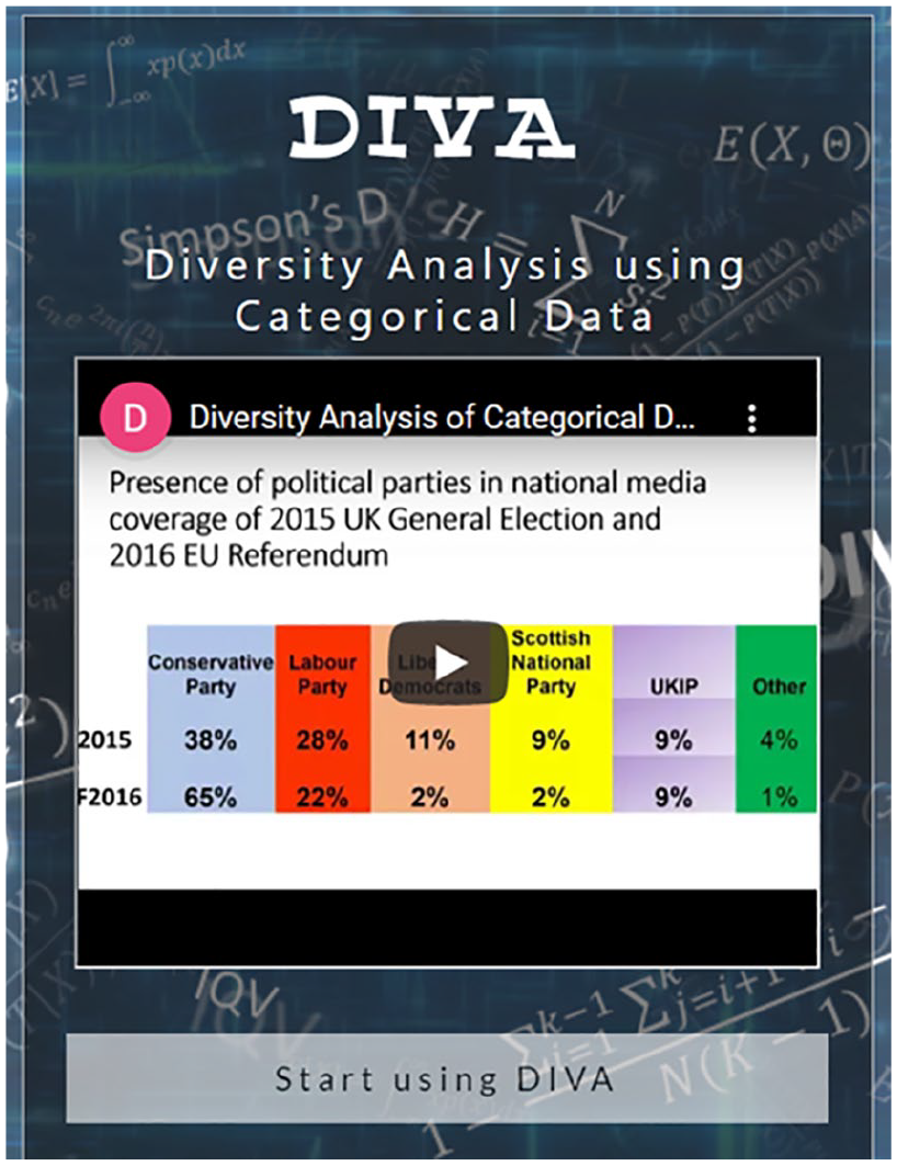
Diversity analysis online tool.

But any discussion of these technical and methodological matters needs to begin with consideration of the wider conceptual parameters of the media diversity debate. For what may seem a simple equation (i.e. more diversity = more democracy) is a calculus of greater algebraic complexity. The additional equational components include where one looks for diversity, how one defines it, how it is measured and whether it is possible to conceive of excessive diversity?

Dimensions of diversity

The importance of media diversity for democracy has been widely recognised and documented, as too have the threats to it from a range of centripetal and centrifugal forces (for synoptic accounts over time, see De Bens, 1998; Dominick & Pierce, 1976; Joris et al., 2020; Loecherbach et al., 2020; McQuail & Van Cuilenburg, 1983). Indeed, one of the key challenges of media policy remains how to mitigate the impact of these forces (McQuail, 2007). From a supply side, centripetal tendencies of markets have long been recognised as leading to greater concentration of media ownership in the hands of fewer corporations, and growing output homogeneity. From the demand side, market pricing, digital divides, and inequalities in public access to media, have been identified as undermining the needs of citizens (Van Cuilenburg, 2000). At the same time, centrifugal forces are said to undermine a sense of a shared common sphere for citizens as evidenced by the rise of algorithmic information provision, and digital filter bubbles and echo chambers (see Möller et al., 2018; Powers & Benson, 2014; Stroud, 2011). These forces threaten citizens’ opportunities to access the resources needed to participate fully and effectively in national democratic life, making democracy all the poorer.

Concerns about the diversity of media content and representation intersect with supply and demand side questions, particularly when assessing the impact that different media environments have upon the plurality of public discourse. In discussions about content diversity, attention has focussed upon (but is not restricted to) the measurement of source diversity (i.e. which individuals and institutions gain greatest prominence in media representations) and content diversity (i.e. what issues and frames receive greatest prominence; Voakes et al., 1996).

These disparate concerns highlight the need to appreciate the different conceptual levels in the analysis of media diversity. McQuail and Van Cuilenburg (1983) distinguish between the macro level (‘the entire media “system” of a society’), the meso level (‘a sector within a media system’) and the micro level (‘the individual media organisation or outlet’; p. 151). Roessler (2008) also uses these terminological distinctions but in a somewhat different way, drawing a useful distinction between ‘diversity’ (‘the variety or breadth of media content’) and ‘diversification’ (‘the supply side of media firms’; p. 467). In his analysis, the macro-level attends to ‘the media system and its overall structure (Roessler, 2008, p. 465), the meso-level (‘single media outlets in a given media system’) and the micro level (the coverage ‘of issues and protagonists’).

These different analytical frames in turn raise the question: at what level should assessments about the content diversity be made? Should the focus be on diversity within particular media outlets (variously referred to as ‘internal’, ‘vertical’ or ‘intra-media’ diversity) or on cumulative diversity across media sectors or systems (referred to as ‘external’, ‘horizontal’ or ‘inter media’ diversity; Van Cuilenburg, 2008, pp. 28–29)? There are tensions between these perspectives as ‘[t]he more intra diverse content packages are, the less inter diverse they can be – and vice versa’ (Van Cuilenburg, 2000, p. 28). Understanding these alternate stances is also valuable for understanding distinctions within and between national media systems. For example, UK national newspapers are renowned for their political partisanship and party alignment, whereas public service broadcasters are required to demonstrate due impartiality and balance in their coverage of the political sphere. The justification for the former is found in appeals to ‘external diversity’ (i.e. citizens can choose a newspaper that most suits their political palate in a competitive marketplace), whereas the rationale for the latter relates to the importance of securing ‘internal diversity’ (because of the centrality of broadcasting channels as providers of entertainment and information and, in the case of the BBC, its public funding).

One of the challenges of research in media diversity is to understand the nature and conditions of these intersecting levels and concepts. Voakes et al. (1996) used an empirical case study to assert that ‘the common assumption that source diversity begets content diversity is fallacious. They sometimes accompany each other, but they appear to vary independently of each other’ (p. 591). Other studies also challenge assumptions that diversity of ownership guarantees greater plurality of content as media owners sometimes seek to differentiate content provision across outlets in their portfolio to increase overall consolidation of market share (Roessler, 2008, p. 478).

Diversity can sometimes be too much of a good thing. Just as a non-diverse mainstream media can constrain the parameters of public understanding, so excessive diversity can create a disorientating diffuseness in public discourse (Gitlin, 1998). This in turn begs the question as to what normative principles should be applied when appraising media diversity. One approach orientates to the concept of ‘reflective diversity’ and measures the goodness-of-fit between media representations and known population distributions and preferences. The other is ‘open diversity’ which is more concerned with the opinion-leading potential of the media in social terms and their responsibility to extend and pluralise public debate, regardless of underlying social configurations. Van Cuilenberg (2000) notes the tensions between reflective and open diversity: ‘Media fully reflecting social preferences inevitably ill perform at openness to a greater variety of different perspectives, social positions and conditions, whereas perfect media openness harms majority positions in favour of minority perspectives, beliefs, attitudes and conditions’ (p. 30). Raeijmaekers and Maeseele (2015) distinguish four normative frameworks, each implying ‘a different conceptual interpretation of media, pluralism, and democracy in general, and media pluralism in specific’ (p. 1051). The first is ‘affirmative diversity’, which sees the media as ‘mirrors of society’ and ‘marketplaces of ideas’. The second is ‘affirmative pluralism’, represented by the metaphor of media as ‘public forums’. Third is ‘critical diversity’, with a focus on the ‘cultural industries’, it highlights the ‘structural inequalities – mostly economic’ – and how they ‘negatively influence media representation’. Finally, there is ‘critical pluralism’ which emphasises the ‘media as ‘sites of struggle’ or ‘fields of contestation’ (pp. 1052–1054). Loecherbach et al. (2020) also identify four dominant normative models present in the wider literature. Our concern here has mainly been with what they term the liberal-aggregative and liberal-individual frameworks, in which citizen have access to a wide variety of views and have equal opportunities to participate (see Loecherbach et al., 2020). It should be noted they also identify deliberative and adversarial/ critical frameworks (see Loecherbach et al., 2020), but these lie outside the scope of this article.

Measure for measure: statistical description of diversity

A shared aspect of all these debates is a concern with questions of accumulation, scale and patterning across media content, contexts, and temporalities. These invite questions of measurement and particularly their statistical summation. In this respect, there is a challenge, as many things that are measured to assess media diversity only attain the nominal level of measurement (e.g. ownership concentration within media markets, gender and ethnicity distributions within creative industries, the prioritisation of certain frames and sources within a chosen issue domain).

This reliance on categorical measures precludes many of the standard measures of variance applied to data that attain ordinal, interval and ratio levels. It also means that many of the statistical analyses of differences and trends in diversity are reliant principally on cross-tabulated comparisons (e.g. Deacon, Downey, Smith, & Wring, 2017; Deacon, Downey, Stanyer, & Wring, 2017; Deacon, & Wring 2017; Wahl-Jorgensen et al., 2017). Such tabulations have undeniable analytical value: it is important to demonstrate where observed differences or confluences occur. But their use and interpretability rapidly degrade the more data points and categories that are introduced and as the analysis extends into multivariate dimensions. This is particularly regrettable for the analysis of diversity as it limits opportunities to model the relationship between the different conceptualisations outlined earlier (e.g. how the strength in correlation between source and content diversity varies with differential orientation to internal or external diversity norms?).

Rediscovering diversity indices (and recognising their inconsistent labels)

It so happens there exist a range of statistical indices that measure the strength of qualitative variation and are of value in addressing these methodological challenges. These indices have been developed across a variety of disciplines, including botany, economics, sociology and information science, but they are relatively obscure. Several decades ago, the statistician Allen Wilcox (1973) noted that ‘the discussion of the measurement of variation with nominal-scale data is usually conspicuous by its absence’ (p. 325) and we can attest, having trawled dozens of contemporary statistical textbooks in preparing this article, that this remains the case. They are referenced infrequently and their calculation is not supported by major statistical software. There are instances where these measures have been used in the analysis of media performance and diversity, but these occasions are vanishingly small and we contend it is timely for researchers within the field to consider their use and limitations more widely.

In developing our analysis, two interventions have proven particularly valuable in identifying the main indices. The first is Indices of Qualitative Variation and Political Measurement authored by the aforementioned Wilcox (1973). The second is The Conceptualisation and Measurement of Diversity written by McDonald Dimmock (2003). Wilcox’s overview considers the performance of six indices: the deviation from the mode (DM), the mean difference analogue (MDA), the average deviation analogue (ADA), HREL, the variance analogue (VA) and Kaiser’s B. McDonald Dimmock consider nine measures: Simpson’s D, Simpson’s D_z, Kvalseth’s OD, Jung’s H, Shannon’s H, Gleason’s D, Hall and Tideman’s H, Fager’s S and Fager’s NM. The lack of any apparent overlap in the measures discussed is a further indicator of the underdeveloped nature of this statistical field (although, as discussed below, HREL and Shannon’s H are closely linked).

At first sight, both reviews appear to exclude two further indices of qualitative variation that have been used relatively widely. The Herfindahl–Hirschman index (HHI) was developed in economics to measure market concentration and has been applied in several studies of media diversity (e.g. Entman, 2006; Powers & Benson, 2014). The index of qualitative variation (IQV) has achieved some prominence as a diversity measure in sociological research (e.g. Agresti & Agresti, 1978; Marsden, 1987). The apparent exclusion of each from these reviews has different explanations. McDonald Dimmock (2003: 67–68) explain that HHI is mathematically equivalent to Simpson’s D but not as simple to interpret (NB the version of Simpson’s D included in this article produces a diversity measure between 0 and 1 whereas HHI scores can range from nearly 0 to 10,000). The absence of the IQV measure is due to Wilcox labelling it the ‘Variance Analogue’ in his overview. Terminological inconsistency of this kind is a consistent (and confusing) feature of the use of these measures, as are differences in the calculation of some indices with the same name. For example, Shannon’s H (1948), first developed by the information theorist Claud Shannon in the 1940s, is also referred to as the ‘Shannon entropy measure’, the ‘Shannon Weaver index’ and the ‘Shannon Weiner index’ (Spellerberg & Fedor, 2003). It is also often found that H is then standardised equitability, to produce a final statistic between 0 and 1. This is variously referred to as HREL or the Shannon equitability index. Similar confusions exist with Simpson’s D (1949), which is sometimes referred to as Gini–Simpson’s index, and depending on its mode of calculation, can generate figures between 0 and 1, or from 1 and above.

Given the variety of indices, the assessment in this article will focus on the statistical indices deemed by Wilcox, McDonald, Dimmock and other authors to be most effective, stable and easy to use (e.g. see also Tan & Weaver, 2013, p. 778; Teachman, 1980, p. 344). These are: Simpson’s D, HREL, the IQV (aka variance analogue in Wilcox’s typology), the MDA and the DM. All of these measures meet Wilcox’s (1973) requirements that: (1) variation is measured as between 1 and 0; (2) when the distribution of all of the observations are the same, variation is 0 and (3) when all of the observations are equally different, the variation is 1. They also pass the dual-concept requirement identified by McDonald Dimmock (2003). This is that the measures take account of: (1) the range of discrete categorisations within a nominal distribution and (2) the assignment of elements to those categories. With all indices, nominal distributions can be entered as observed values or percentage distributions. In addition, categories that contain zero observations must be included in the calculation as their emptiness says something about the overall diversity of a distribution.

Table 1 outlines the statistical equations we used to calculate each measure (with notation standardised across the various equations). As mentioned earlier, we have developed a web resource that automates these calculations (see https://diva.lboro.ac.uk).

Table 1.

Equations for diversity indices.

Simpson’s D	$1 - \frac{\sum^{} f (f - 1)}{N (N - 1)}$
IQV	$\frac{K (100^{2} - \sum^{} P c t^{2})}{100^{2} (K - 1)}$
HREL	$- \sum_{i = 1}^{k} \frac{f_{i}}{N} \log_{2} \frac{f_{i}}{N}$
MDA	$1 - \frac{\sum_{i = 1}^{k - 1} \sum_{j = i + 1}^{k} \| f_{i} - f_{j} \|}{N (K - 1)}$
DM	$1 - \frac{\sum_{i = 1}^{K} (f_{m} - f_{i})}{N (K - 1)}$

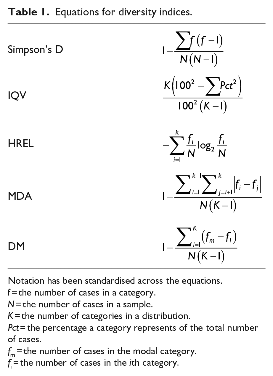
Notation has been standardised across the equations.

f = the number of cases in a category.

N = the number of cases in a sample.

K = the number of categories in a distribution.

Pct = the percentage a category represents of the total number of cases.

f_m = the number of cases in the modal category.

f_i = the number of cases in the ith category.

An illustrative case study of diversity index performance

To assess the use and performance of these selected measures, we used data from media content analyses of three recent UK electoral events: national TV and newspaper reporting of the 2015 United Kingdom General Election (GE2015), the 2016 UK European Union Membership Referendum¹ (REF2016) and the 2017 UK General Election (GE2017).² All studies were conducted by the Centre for Research in Communication and Culture, Loughborough University (see Deacon, Downey, Stanyer, & Wring, 2017; Deacon et al., 2016; Deacon & Wring, 2017). Although discrete studies, they used repeated measures, identical sampling procedures, near identical coding teams and were each subject to inter-coder reliability testing.³ To emphasise, these data are used here solely for illustrative purposes, to assess how different measures perform and how they can be used in empirical analysis to appraise and compare diversity in nominal data across different contexts.

To assess the performance of the selected indices, we compared their measurement of ‘source diversity’ in the coverage of these three electoral events. Our measure of source diversity was the frequency of appearance of quoted party-political representatives across the entirety of each campaign sample.

Categorisation effects

The first issue we examined was whether different category groupings of the same data sets changed diversity scores – that is, could we identify any categorisation effects? As noted, one of McDonald Dimmock’s (2003) ‘dual concept’ requirements for evaluating a diversity measure is that the calculation takes account of the range of discrete categorisations within a nominal distribution, thereby opening up the potential for the comparison of diversity scores for distributions with different numbers of categories. However, if diversity scores appear to be affected by the range of categorisations, such practices need to be questioned.

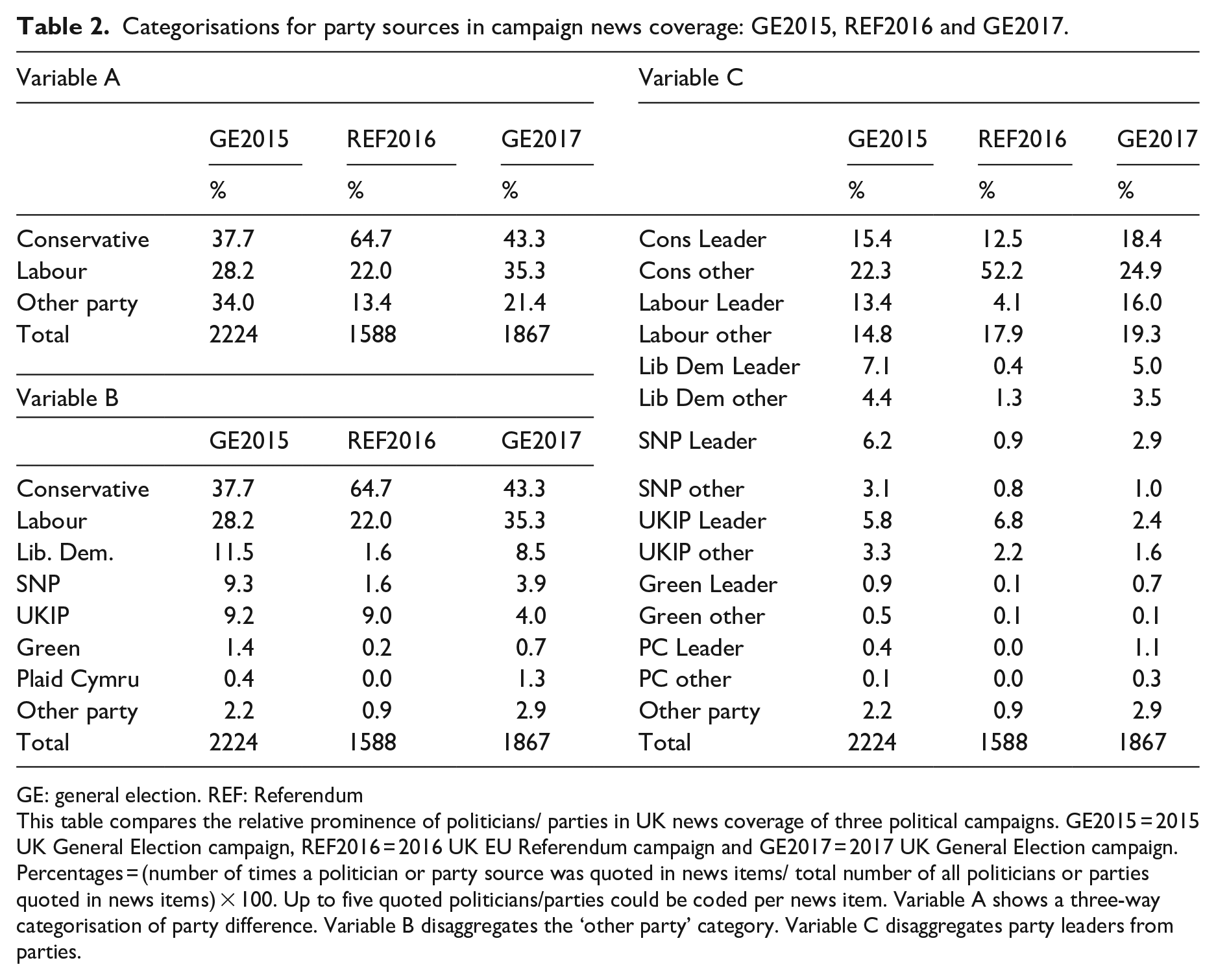
To analyse this aspect, we categorised source diversity distributions for the three campaigns in three ways (see Table 2). Variable A differentiated between sources from the two main parties and placed ‘all other parties’ in a single category. Variable B elaborated the ‘all other parties’ category to produce a distribution with eight party categories. Variable C extended this further, making a distinction between the appearance of ‘party leaders’ and ‘all other party sources’ for the seven main UK political parties and a remaining category for ‘all other party sources’, producing 15 categories. The categorisations and the data distributions for each are set out in Table 2. Table 3 provides the statistical summary for source diversity in each campaign and categorisation, using the five selected diversity indices.

Table 2.

Categorisations for party sources in campaign news coverage: GE2015, REF2016 and GE2017.

Variable A				Variable C
	GE2015	REF2016	GE2017		GE2015	REF2016	GE2017
	%	%	%		%	%	%
Conservative	37.7	64.7	43.3	Cons Leader	15.4	12.5	18.4
Labour	28.2	22.0	35.3	Cons other	22.3	52.2	24.9
Other party	34.0	13.4	21.4	Labour Leader	13.4	4.1	16.0
Total	2224	1588	1867	Labour other	14.8	17.9	19.3
				Lib Dem Leader	7.1	0.4	5.0
Variable B				Lib Dem other	4.4	1.3	3.5
	GE2015	REF2016	GE2017	SNP Leader	6.2	0.9	2.9
Conservative	37.7	64.7	43.3	SNP other	3.1	0.8	1.0
Labour	28.2	22.0	35.3	UKIP Leader	5.8	6.8	2.4
Lib. Dem.	11.5	1.6	8.5	UKIP other	3.3	2.2	1.6
SNP	9.3	1.6	3.9	Green Leader	0.9	0.1	0.7
UKIP	9.2	9.0	4.0	Green other	0.5	0.1	0.1
Green	1.4	0.2	0.7	PC Leader	0.4	0.0	1.1
Plaid Cymru	0.4	0.0	1.3	PC other	0.1	0.0	0.3
Other party	2.2	0.9	2.9	Other party	2.2	0.9	2.9
Total	2224	1588	1867	Total	2224	1588	1867

GE: general election. REF: Referendum

This table compares the relative prominence of politicians/ parties in UK news coverage of three political campaigns. GE2015 = 2015 UK General Election campaign, REF2016 = 2016 UK EU Referendum campaign and GE2017 = 2017 UK General Election campaign. Percentages = (number of times a politician or party source was quoted in news items/ total number of all politicians or parties quoted in news items) × 100. Up to five quoted politicians/parties could be coded per news item. Variable A shows a three-way categorisation of party difference. Variable B disaggregates the ‘other party’ category. Variable C disaggregates party leaders from parties.

Table 3.

Macro-diversity scores for news coverage of political parties in the GE2015, REF2016 and GE2017 campaigns.

	Campaign	HREL	D	IQV	MDA	DM
Variable A	GE2015	0.993	0.662	0.993	0.907	0.944
	REF2016	0.804	0.516	0.773	0.487	0.53
(3 categories)	GE2017	0.965	0.643	0.963	0.781	0.851
Variable B	GE2015	0.761	0.747	0.854	0.396	0.712
(8 categories)	REF2016	0.524	0.525	0.600	0.163	0.404
	GE2017	0.670	0.677	0.773	0.308	0.648
Variable C	GE2015	0.828	0.87	0.932	0.442	0.832
	REF2016	0.590	0.673	0.721	0.177	0.512
(15 categories)	GE2017	0.756	0.835	0.894	0.353	0.805

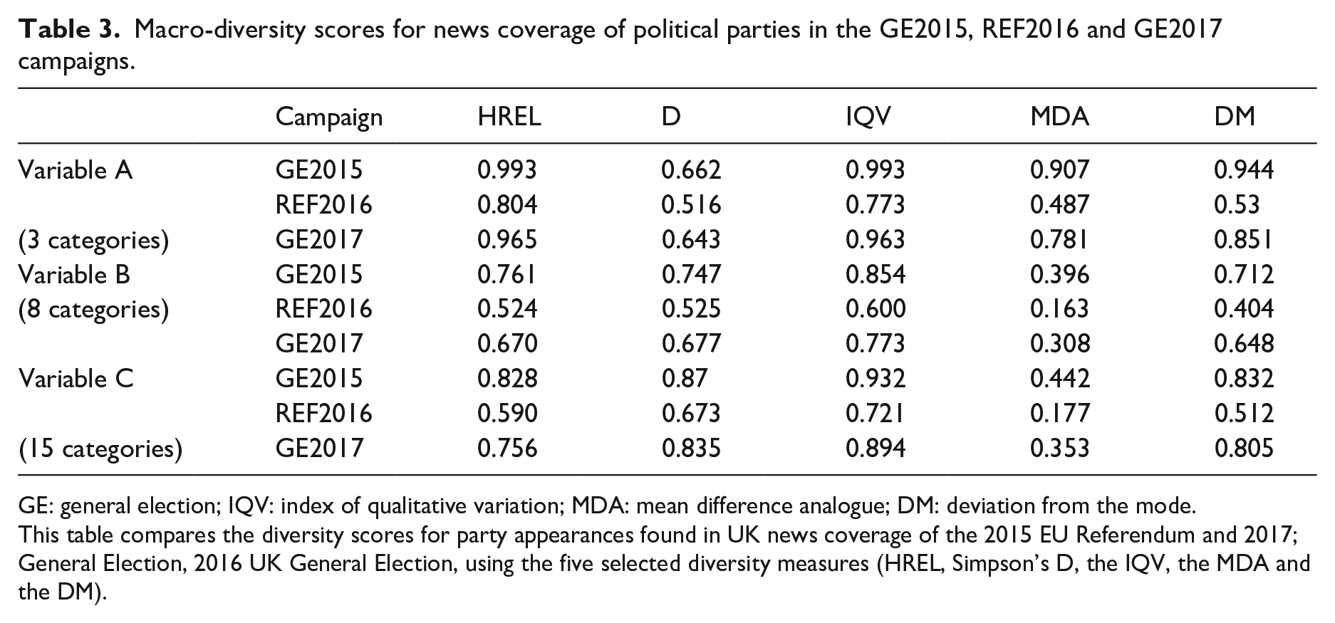
GE: general election; IQV: index of qualitative variation; MDA: mean difference analogue; DM: deviation from the mode.

This table compares the diversity scores for party appearances found in UK news coverage of the 2015 EU Referendum and 2017; General Election, 2016 UK General Election, using the five selected diversity measures (HREL, Simpson’s D, the IQV, the MDA and the DM).

In broad terms, the diversity measures for each categorisation of the three campaigns tell a consistent story: all indicate that news coverage of the 2015 UK General Election had the highest source diversity, followed by the 2017 UK General Election and then the 2016 EU Referendum. Closer analysis reveals variation both within and between diversity measures. This variation is not consistent, but there are some tendencies. The IQV results were either the highest or joint highest in seven of the nine cases, and the second highest in the remainder. At the other end, MDA scores were the lowest in seven of the nine cases, and second lowest in the remainder. The remaining three measures fluctuated more inconsistently in positioning. D scores were second highest in five cases, but the lowest in two of the remainder, DM scores were never higher than third in the rankings, HREL results varied most widely in terms of rankings.

The measures also reveal different levels of stability across the categorisation options. To assess this aspect, we calculated the average of all permutations of the absolute differences for the categorisations of each measure, for each election.⁴ By this test, IQV showed least average variation (0.112), followed by D (0.124), DM (0.125) and HREL (0.179). MDA was a striking outlier by this measure, producing an average variation of 0.291.

We identify four implications to these findings. First, even with standardised measures, it is not possible to compare across indices, as certain measures are inclined to produce higher values than others, even when the categorical range is the same. Second, the resilience of different diversity measures to categorisation effects varies, but there seems to be such volatility in the MDA that it raises serious questions about its reliability as a diversity measure. Third, there are risks in comparing diversity scores where different categorisations have been used. For example, if we wanted to compare source diversity in GE2015 and GE2017 news coverage and used the variable B, IQV score for the former (0.854) and the variable C, IQV score for the latter (0.894), we would erroneously conclude that coverage of the 2017 General Election had greater source diversity, whereas all the like-for-like comparisons show the reverse to be the case. Fourth, recognition of this shows that diversity scores need to be assessed contextually and it is problematic to try and conceive of any abstracted statistical thresholds for ascertaining ‘high’, ‘medium’ or ‘low’ diversity.

This last point has implications for a tendency we have noted within the economics literature around the application of the Herfindahl–Hirschman Index in the measurement of market competition. As noted earlier, the HHI is the direct mathematical equivalent of Simpsons’ D, but produces results from close to 0–10,000 in which the lower a score is, the greater the diversity of a distribution. The US government agencies currently apply an abstracted standard that judge markets with an HHI below 1500 as ‘unconcentrated’, with an HHI between 1500 and 2500 as ‘moderately concentrated’ and an HHI above 2500 above HHI as ‘Highly concentrated’ (US Department of Justice, 2018). If we were to use the GE2015 distribution as a proxy for a measure of concentration within an imaginary market, the variable B categorisation would produce an HHI score of 2529, and the variable C, an HHI of 1303. In other words, applying the abstracted US government agency criteria, the variable B categorisation would indicate a ‘highly concentrated’ market and the variable C categorisation an ‘unconcentrated’ one.

Diversity averaging: beyond the ‘First past the post’ and ‘horses for courses’ standoff

Where does this recognition of the variance across diversity indices leave us in terms of selecting a measure? We discern two approaches within the limited literature on diversity indices. The first might be labelled ‘the first past the post’ approach and involves asserting that one measure is the ‘best’ overall measure (e.g. Tan & Weaver, 2013). The second, can be termed the ‘horses for courses’ approach and claims that some measures are better for addressing specific questions related to diversity and some for others (e.g. Teachman, 1980, p. 344). In our view, the first approach presents a question that is difficult to resolve, whereas, the second poses a question that is difficult for non-specialists to understand. A neat solution to this would be to develop an integrated measure that averages a composite of selected measures. Straightforward averaging might seem crude, but it is a technique that is commonly used in areas such as economic forecasting and is recognised as improving forecast accuracy (e.g. Clemen, 1989).

For the constituent elements of this measure we recommend using the four diversity measures shown to perform most consistently (HREL, D, IQV and DM). We propose naming this composite measure the DIVa and have included a facility for its automated computation on the web resource developed in conjunction with this article. The DIVa scores for all media in the three campaigns were (variable A) 0.898, 0.656, 0.855; (variable B) 0.768, 0.513, 0.692 and (variable C): 0.865, 0.624, 0.822. Once again, we calculated the average of all permutations of the absolute differences, for each election and found DIVa had a lower averaged variation than all single measures (0.097). This suggests that the combination of measures in its calculation ameliorates the categorisation effects noted with individual measures.

From description to inference: the need for innovation

All diversity measures are descriptive statistics and as such are limited in the extent to which they can be extrapolated and compared. Any variations – such as the differences shown in the three campaigns through our illustrative example – may reveal something important or they may just be a product of the random fluctuation that occurs in any form of sampling.

Statistical inference permits two core tasks: estimating ‘true’ population parameters from descriptive measures and hypothesis testing (Deacon et al., 2021). Wilcox (1973) notes that it is necessary to gain knowledge of the sampling distributions of diversity indices ‘if one hopes or intends to apply procedures of statistical inference’ (p. 340). In this respect, the already limited literature on the measurement of qualitative diversity is nearly silent. Neither McDonald Dimmock (2003) nor Wilcox (1973) provide guidance on statistical testing and most studies that use diversity indices do not include significance tests. On the rare occasions such tests appear, it is difficult to identify the procedures that have been used (e.g. Humprecht & Esser, 2017) or their application requires advanced understanding and operationalisation of statistical formulae (e.g. Agresti & Agresti, 1978, pp. 211–229).

In this section, we propose the use of ‘bootstrapping’ and ‘permutation testing’ techniques to address the twin challenges of drawing population estimates and hypothesis testing from observed diversity scores. Bootstrapping can be used to calculate confidence intervals for population estimates (i.e. the range in which the ‘true’ population value likely to lie on the basis of sampled observations). Permutation testing can be used for hypothesis testing (i.e. calculating whether observed differences in descriptive measures are statistically significant). Both approaches have long prehistories (e.g. Fisher, 1935), but it is only with the accessibility to powerful computer technology that their application has become widespread (Mooney, 1996). Both deploy resampling techniques to generate the necessary sampling distributions needed for inferential statistical work.

Bootstrapping

The name ‘bootstrapping’ is taken from the phrase ‘pulling oneself by one’s own bootstraps’ and calculates population distributions by using the information you have available: that is, your sample data. The process involves generating large numbers of random resamples (with replacement) from this data set. When we talk of sampling ‘with replacement’ we are describing a process whereby once a value is selected for inclusion in a resample, it is returned to the selection process thereby permitting the possibility that it might again be resampled randomly.

Bootstrapping for the diversity measures discussed here involved generating a 1000 resamples with replacement of the samples for GE2015, REF2016 and GE2017. All selected diversity indices were then calculated for each resample and ranked from highest to lowest. This produced a bootstrap distribution that is used as our sample distribution. To calculate the 95% confidence interval with 1000 resamples (p < 0.05), we identified the 26th lowest ranked value and the 975th highest ranked value for each diversity measure. Table 4 shows the CIs for DIVa, D, HREL, IQV and DM.

Table 4.

95% confidence intervals estimated for GE2015, REF2016 and GE2017 variable C source diversity scores.

	Diversity score	95% CI
GE2015
DIVa	0.865	0.834–0.915
D	0.87	0.84–0.893
HREL	0.828	0.816–0.919
IQV	0.932	0.908–0.963
DM	0.832	0.753–0.902
REF2016
DIVa	0.624	0.572–0.746
D	0.673	0.587–0.744
HREL	0.59	0.595–0.758
IQV	0.721	0.663–0.835
DM	0.512	0.434–0.653
GE2017
DIVa	0.822	0.792–0.878
D	0.835	0.8–0.864
HREL	0.756	0.748–0.866
IQV	0.894	0.87–0.935
DM	0.805	0.726–0.869

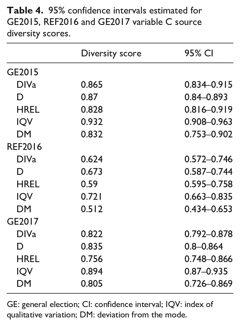
GE: general election; CI: confidence interval; IQV: index of qualitative variation; DM: deviation from the mode.

Permutation testing

Permutation testing shares similarities to bootstrapping, in that it involves the estimation of population distributions by multiple resampling of observed values. The principal differences are that it is used to compare differences between two variables (hence its role in hypothesis testing) and the resampling is conducted without replacement (i.e. when a value is resampled it is excluded from subsequent selections). The procedure starts by considering ‘the value of the statistic actually observed in the study’ (Hesterberg et al., 2007, Section 16.42). In our example, this would be comparing the observed differences in two-way comparisons of QV scores for source diversity in media coverage of different campaigns and it is computed by calculating the absolute value between the two diversity scores (e.g. the absolute difference in the values found for Simpson’s D values found for GE2015 and REF2018 is 0.197). We then construct a null hypothesis – that is, that the observed difference between the two scores is likely to be the product of chance and cannot be deemed statistically significant. The next step requires the creation of a sampling distribution that ‘this statistic would have if the effect were not present in the population’ (Hesterberg et al., 2007, Section 16.40), and then comparing the observed statistic to this distribution. If the value sits centrally in the distribution there is a high chance it occurred by chance, but the further away from the centre it sits, the greater the probability ‘that something other than chance is operating’.

The sampling distribution described above is known as the permutation distribution and assumes that the null hypothesis is true (i.e. ‘that the two groups’ code counts are identically distributed, or that the grouping variable does not influence the outcome’ (Collingridge, 2013, p. 89)). To construct this distribution, the observed distributions in two samples are shuffled into a pooled sample from which two new samples are created that replicate the original sample structures. These twinned samples are created by randomly selecting sample units that are not then returned to the pooled data (i.e. resampled without replacement). The measure under assessment (e.g. each of the selected diversity scores) is then calculated for both resamples and the value of the second resample is subtracted from the first, to produce a positive or negative value. This process is repeated multiple times to produce the permutation distribution (1000 resamples should be seen as a lower limit). The observed difference is then mapped onto the permutation distribution to gain a p value. This is calculated as the proportion of resampled values that give a result as high as the observed difference being tested. For example, we have noted that the difference in the Simpsons’ D diversity score for GE 2015 and REF2016 was 0.197. Resampling results found 13 of the 1000 resamples produced a value the same or higher, which means the estimated p-value is 0.013 (13/1000).

There is one important caveat to be borne in mind when using this method. Significance testing will not operate for the comparison of variables with three or fewer categories. This is because if there are less than 20 possible permutations with two independent variables, p ⩽ 0.05 can never be attained (see Ludbrook & Dudley, 1998, p. 130).

Table 5 shows the results of two-way permutation testing for each of the three media campaigns used for our illustrative case study. The results show the degree of statistical confidence we can have that these observed sample differences between paired media campaigns (i.e. GE2015 and REF2016; GE2017 and REF2016; GE2015 and GE2017) are indicative of actual differences in the wider population. The findings reveal that the observed differences in source diversity between GE2015 and REF2016 for all indices are statistically significant (using p ⩽ 0.05 to determine statistical significance), whereas the differences between GE2015 and GE2017 are not. The results also show that differences between GE2017 and REF2016 are statistically significant for D, IQV and DM, but not for HREL (p = 0.07). This raises a further question about the use of single diversity measures, as this example suggests that the determination of statistical significance can be affected by the choice of measure. This adds strength to the case for developing a composite measure like DIVa, as it offers a way of resolving those instances where significance tests for different measures reach discrepant conclusions.

Table 5.

Hypothesis testing: variable C comparisons.

Comparison of GE2015 and REF2016	GE2015	REF2016	Absolute difference
DIVa	0.865	0.624	0.241*
D	0.870	0.673	0.197*
HREL	0.828	0.590	0.238*
IQV	0.932	0.721	0.211*
DM	0.832	0.512	0.320*
Comparison of GE2017 and REF2016	GE2017	REF2016	Absolute difference
DIVa	0.822	0.624	0.198*
D	0.835	0.673	0.162*
HREL	0.756	0.590	0.166
IQV	0.894	0.721	0.173*
DM	0.805	0.512	0.293*
Comparison of GE2015 and GE2017	GE2015	GE2017	Absolute difference
DIVa	0.865	0.822	0.043
D	0.870	0.835	0.035
HREL	0.828	0.756	0.072
IQV	0.932	0.894	0.037
DM	0.832	0.805	0.028

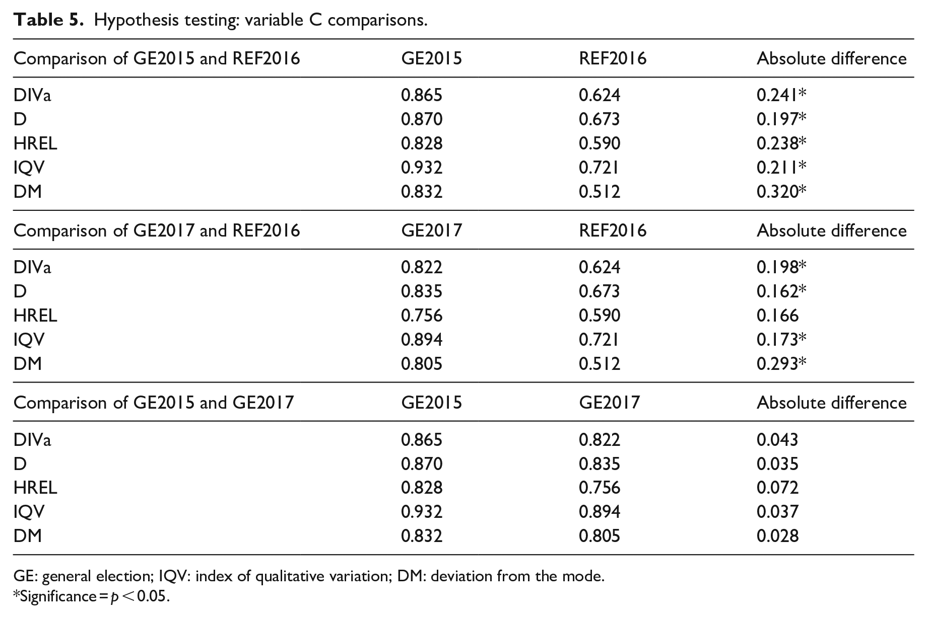
GE: general election; IQV: index of qualitative variation; DM: deviation from the mode.

Significance = p < 0.05.

Conclusion

This article has reviewed the key conceptual debates about media diversity and identified a major methodological challenge: how can statistical variance be modelled across these different conceptual frameworks when so many of the core measures only attain the nominal level of measurement?

We suggest a valuable way forward is to make greater use of indices of qualitative variation that have been developed across diverse disciplines. These measures are not part of the statistical mainstream and this obscurity is compounded by the confusion and inconsistencies surrounding their labelling. One of the purposes of this article has been to identify and resolve these confusions.

We assessed the performance of five diversity indices: Simpsons’ D, the IQV, HREL, the MDA and the DM. Five broader points need to be drawn from this assessment.

First, these measures are most appropriate for the analysis of ‘open’ diversity – that is, the extent to which values are evenly spread across nominal categories. They are less useful for appraising ‘reflective diversity’ – that is, the extent to which the dispersion of values in one distribution mirrors that of another. This is because even if two diversity scores are very similar, there is no guarantee that the constituent values disperse in a similar way across the categories. For this reason, measuring reflective diversity requires the adaption of other correlational statistical measures (see Deacon et al., 2020 for an example of this in practice). However, these diversity indices do have a value in assessing the extent to which news organisations orientate to internal or external diversity goals (i.e. the extent to which they see their role as providing pluralistic coverage within their content, or providing a distinctive perspectives that contribute to pluralism across different outlets).

Second, these measures can just as readily be applied to ‘demand side’ diversity questions as they can to ‘supply side’ issues (e.g. the ‘exposure diversity’ of citizens to different media outlets). The case study we present of ‘source diversity’ in political news coverage is offered purely for illustrative purposes.

Third, it is not appropriate to think about abstract statistical benchmarks for what might indicate ‘good’, ‘acceptable’ or ‘poor’ levels of diversity (even though some authoritative sources have suggested this can be done). This is partly because some measures tend to give consistently higher diversity scores than others, even when they are standardised to produce scores between 1 and 0. Furthermore, there are clear ‘categorisation effects’ – that is, that diversity scores are affected by the number of categories used. This issue has been signally neglected in the methodological literature to date but means that diversity scores always need to be considered contextually and comparatively. Furthermore, these comparisons must use the same diversity measure and the same categorisation structure to ensure that any observed differences are not an artefact of failing to compare like-with-like.

Fourth, our evaluation led us to recommend the development of a new averaged measure of the most stable diversity indices. This approach is commonly found in financial forecasting and recognised to improve forecast accuracy. We label this new composite measure the DIVa and show that it helps avoid the contentiousness of claiming that one measure is superior to others (the ‘first past the post’ argument) and the complexities of determining which measures are best for which scenarios (the ‘horses for courses’ argument). The measure also addresses, at least partially, the two problems noted above, in that it flattens out fluctuations across different measures, and reduces categorisation effects.

Finally, we suggest two ways in which statistical inferences can be made from these descriptive statistical methods (which is another neglected issue in the available literature). To estimate confidence intervals, we recommend ‘bootstrapping’ resampling methods to construct sampling distributions from observed values. For hypothesis testing, we suggest ‘permutation testing’ resampling to create a null hypothesis distribution to calculate the probability that observed differences between two diversity scores occurred by chance. The latter exercise also reveals a further value to the new DIVa measure, as it helps to arbitrate those occasions when certain diversity indices suggest there is a significant difference between two data distributions and other indices, do not.

All of these methods demand computational assistance and the absence of an accessible resource to perform these tasks has been a major hindrance to the wider application and evaluation of diversity measures. In developing this article, we created a computational resource to automate these tasks. The fruits of this activity are now offered as an online resource to encourage further investigation into the value of the quantification of qualitative variation in communication research.

Footnotes

Acknowledgements

The authors would like to thank Orange Gao and Peter Dean of Business Intelligence and Strategy Ltd and Dr Adrian Leguina, School of Social Sciences, Loughborough University for their assistance in developing the conceptual and technical aspects of this paper.

ORCID iD

David Deacon

Notes

Author biography

David Deacon is Professor of Communication and Media Analysis at the Centre for Research in Communication and Culture, Loughborough University.

James Stanyer is Professor of Communication and Media Analysis at the Centre for Research in Communication and Culture, Loughborough University.

References

Agresti

(1978). Statistical analysis of qualitative variation. Sociological Methodology, 9, 204–237.

British Broadcasting Corporation. (2018). Editorial guidelines, section 4: Impartiality. https://www.bbc.com/editorialguidelines/guidelines/impartiality/guidelines

Collingridge

(2013). A primer on quantitized data analysis and permutation testing. Journal of Mixed Methods Research, 7(1): 81–97. https://doi.org/10.1177/1558689812454457

Clemen

(1989). Combining forecasts: A review and bibliography with discussion. International Journal of Forecasting, 5(4), 559–608.

Deacon

Downey

Smith

Wring

(2017). Two parts policy, one part process: News media coverage of the 2017 General Election. In Mair

Clark

Fowler

Snoddy

Tait

(Eds.), Brexit, trump and the media (pp. 367–71). Abramis.

Deacon

Downey

Stanyer

Wring

(2017). The media campaign: The issues and personalities who defined the election. In Wring

Mortimore

Atkinson

(Eds.), Political communication in Britain: Polling, campaigning and media in the General Election 2015 (pp. 183–196). Palgrave Macmillan.

Deacon

Pickering

Golding

Murdock

(2021). Researching communications: A practical guide to media and cultural analysis (3rd ed.). Bloomsbury.

Deacon

Wring

(2017c). One party, two issues: UK news media reporting of the EU referendum. In Mair

Clark

Fowler

Snoddy

Tait

(Eds.), Brexit, trump and the media (pp. 36–44). Abramis.

Deacon

Wring

Vaccari

Smith

(2020). Here, there and everywhere? Brexit and mainstream news coverage during the 2019 General Election. In Mair

Clark

Fowler

Snoddy

Tait

(Eds.), Brexit, Boris, and the media (pp. 27–35). Abramis.

10.

De Bens

(1998). Television programming: More diversity, more convergence. In Brants

Hermes

De Bens

(Eds.), The media in question: Popular cultures and public interests. SAGE.

11.

Dominick

J. R.

Pierce

M. C.

(1976). Trends in network primetime programming, 1953-1974. Journal of Communication, 26, 70–80.

12.

Entman

(1989). Democracy without citizens: Media and the decay of American politics. Oxford University Press.

13.

Entman

(2006). Punctuating the homogeneity of institutionalized news: Abusing prisoners at Abu Ghraib versus killing civilians at Fallujah. Political Communication, 23(2), 215–224. https://doi.org/10.1080/10584600600629844

14.

Fisher

R. A.

(1935). The design of experiments (3rd ed.). Oliver & Boyd.

15.

Gitlin

(1998). Public sphere or public sphericules? In Liebes

Curran

(Eds.), Media, ritual, identity (pp. 168–175). Routledge.

16.

Habermas

(2006). Political communication in media society: Does democracy still enjoy an epistemic dimension? The impact of normative theory on empirical research. Communication Theory, 16, 411–426.

17.

Hesterberg

Moore

Monaghan

Clipson

Epstein

Craig

(2007). Bootstrap methods and permutation tests. In Moore

McCabe

Craig

(Eds.), Introduction to the practice of statistics (6th ed., pp. 16.1–16.58). W. H. Freeman.

18.

Humprecht

Esser

(2017). Diversity in online news. Journalism Studies, 19(12), 1825–1849. https://doi.org/10.1080/1461670X.2017.1308229

19.

Joris

De Grove

Van Damme

De Marez

(2020). News diversity reconsidered: A systematic literature review unravelling the diversity in conceptualizations. Journalism Studies, 21(13), 1893–1912. https://doi.org/10.1080/1461670X.2020.1797527

20.

Loecherbach

Moeller

Trilling

van Atteveldt

(2020). The unified framework of media diversity: A systematic literature review. Digital Journalism, 8(5), 605–642. https://doi.org/10.1080/21670811.2020.1764374

21.

Ludbrook

Dudley

(1998). Why permutation tests are superior to T and F tests in biomedical tesearch. The American Statistician, 52(2), 127–132.

22.

Marsden

(1987). Core discussion networks of Americans. American Sociological Review, 52, 122–131.

23.

McCann

(2013). The diversity policy model and assessment of the policy. SAGE Open, 3(2). https://doi.org/10.1177/2158244013492780

24.

McDonald

Dimmock

(2003). The conceptualisation and measurement of diversity. Communication Research, 30(1), 60–79. https://doi.org/10.1177/0093650202239026

25.

McQuail

(2007). Revisiting diversity as a media policy goal. In Meier

Trappel

(Eds.), Power, performance and politics (pp. 41–58). Nomos.

26.

McQuail

Van Cuilenburg

(1983). Diversity as a media policy goal: A strategy for evaluative research and a Netherlands case study. Gazette, 31(3), 145–162.

27.

Möller

Trilling

Helberger

van Es

(2018). Do not blame it on the algorithm: An empirical assessment of multiple recommender systems and their impact on content diversity. Information, Communication & Society, 21(7), 959–977. https://doi.org/10.1080/1369118X.2018.1444076

28.

Mooney

(1996). Bootstrap statistical inference: Examples and evaluations for political science. American Journal of Political Science, 40(2), 570–602.

29.

Powers

Benson

(2014). Is the Internet homogenizing or diversifying the news? External pluralism in the U.S., Danish, and French press. The International Journal of Press/politics, 19(2), 246–265. https://doi.org/10.1177/1940161213519680

30.

Raeijmaekers

Maeseele

(2015). Media, pluralism and democracy: What’s in a name? Media, Culture & Society, 37(7), 1042–1059. https://doi.org/10.1177/0163443715591670

31.

Roessler

(2008). Media content diversity: Conceptual issues and future directions for communications research. In: Beck

C. S.

(Ed.) Communication yearbook 31 (pp. 464–520). Lawrence Erlbaum.

32.

Shannon

(1948). A mathematical theory of communication. Bell System Technical Journal, 27, 379–423.

33.

Simpson

E. H.

(1949). Measurement of diversity. Nature, 163, Article 688.

34.

Spellerberg

Fedor

(2003). A tribute to Claude Shannon (1916 – 2001) and a plea for more rigorous use of species richness, species diversity and the ‘Shannon-Weiner’ Index. Global Ecology and Biogeography, 12(3), 177–179. https://doi.org/10.1046/j.1466-822X.2003.00015.x

35.

Stroud

N. J.

(2011). Niche news: The politics of news choice. Oxford University Press.

36.

Tan

Weaver

(2013). Agenda diversity and agenda setting: From 1956 to 2004. Journalism Studies, 14(6), 773–789. https://doi.org/10.1080/1461670X.2012.748516

37.

Teachman

(1980). Analysis of population diversity: Measures of qualitative variation. Sociological Methods and Research, 8, 341–362.

38.

US Department of Justice (2018) ‘Herfindahl-Hirschman Index.’ https://www.justice.gov/atr/herfindahl-hirschman-index (accessed 1 April 2021).

39.

Van Cuilenburg

(2000). Media diversity, competition and concentration: Concepts and theories. In De Bens

, (Ed.), Media Between Culture and Commerce (Vol 4, pp. 25–54). Changing Media – Changing Europe Series. Intellect.

40.

Voakes

Kapfer

Kurpius

Shano-yeon Chern

(1996). Diversity in news: A conceptual and methodological framework. Journalism & Mass Communication Quarterly, 73(3), 582–593.

41.

Wahl-Jorgensen

Berry

Garcia-Blanco

Bennett

Cable

(2017). Rethinking balance and impartiality in journalism? How the BBC attempted and failed to change the paradigm. Journalism, 18(7), 781–800. https://doi.org/10.1177/1464884916648094

42.

Wilcox

(1973). Indices of qualitative variation and political measurement. Western Political Quarterly, 26(2), 325–343.

Media diversity and the analysis of qualitative variation

Abstract

Keywords

Introduction

Dimensions of diversity

Measure for measure: statistical description of diversity

Rediscovering diversity indices (and recognising their inconsistent labels)

An illustrative case study of diversity index performance

Categorisation effects

Diversity averaging: beyond the ‘First past the post’ and ‘horses for courses’ standoff

From description to inference: the need for innovation

Bootstrapping

Permutation testing

Conclusion

Footnotes

Acknowledgements

ORCID iD

Notes

Author biography

References