Sage Journals: Discover world-class research

Abstract

Objective

To develop and deploy a deep-learning system for automatic NICE classification of colorectal lesions that delivers real-time assistance, incorporates withdrawal-speed monitoring, and shortens the learning curve for endoscopists.

Methods

A total of 2605 colonoscopic images from three hospitals were used for training/testing, with an independent external set of 99 images for validation. Three CNN models (EfficientNet, ResNet50, VGG19) and three Transformer models (ViT, Swin, CvT) were fine-tuned via transfer learning and compared. Model decisions were explained by Grad-CAM, Guided Grad-CAM and SHAP. The best model was converted to ONNX for cross-platform deployment (>50 FPS) and combined with a perceptual-hash/Hamming-distance algorithm to visualize and alarm withdrawal speed.

Results

EfficientNet achieved the best performance (internal accuracy 0.910, F1 = 0.916). On the external set it reached a macro-average AUC of 0.994 with precision 0.936 and recall 0.918. Compared with endoscopists, the model matched or exceeded sensitivity/specificity for NICE 2 and NICE 3. After ONNX conversion, frame-level inference exceeded 50 FPS, and excessive withdrawal speed triggered yellow/red warnings.

Conclusion

This study is the first to integrate high-accuracy EfficientNet-based NICE classification, comprehensive explainability, and real-time withdrawal-speed monitoring into an ONNX-based multi-terminal system. The tool shows strong potential to improve optical diagnosis consistency for early colorectal cancer and to accelerate training of novice endoscopists.

Keywords

NICE classification colonoscopy CNN transformer withdrawal speed monitoring

Introduction

A study spanning the past 25 years revealed a significant increase in colorectal cancer (CRC) incidence among individuals aged 20 to 49 in Europe, with the annual growth rate reaching as high as 7.9% in the 20 to 29 age group.¹ In China, CRC ranks as the second most common cancer and the fifth leading cause of cancer-related mortality. In 2020 alone, there were 555,000 new cases and 286,000 deaths attributed to CRC. Between 1990 and 2025, CRC incidence has shown a continuous upward trend, with projections indicating further increases in the coming years.²

Colonoscopy is the gold standard for detecting colonic polyps and cancer.^3–5 Most adenomatous polyps and early mucosal carcinomas can be excised using endoscopic techniques such as EMR and ESD. However, for cancers with deep submucosal infiltration, surgical intervention is recommended.^6–8 Although colonoscopy is widely adopted, real-time differentiation of lesion types remains challenging. The narrow-band image international colorectal endoscopic classification(NICE) offers an efficient solution, allowing accurate identification of the histological characteristics of lesions without the need for optical magnification.⁹ This classification is favored by endoscopists for its clarity, but physicians still undergo a learning curve when mastering its application and face issues of assessment consistency.¹⁰

In recent years, the application of artificial intelligence (AI) in various medical fields has been steadily increasing. This includes research utilizing deep learning frameworks to predict the severity of COVID-19 infections,¹¹ as well as the development of AI models and applications based on convolutional neural networks (CNN) for assisting in the interpretation of small-bowel capsule endoscopy.¹² In the realm of automated polyp detection, several studies have developed AI models to distinguish between hyperplastic and adenomatous polyps, providing more precise guidance for clinical resection.^13–15 Despite this, research into distinguishing adenomatous polyps, early mucosal carcinomas, and cancers with deep submucosal infiltration remains insufficient. The NICE classification establishes clear criteria for distinguishing among the three types of colorectal lesions.

The main contributions of the proposed automatic NICE classification model for colorectal lesions is given here.

To train deep learning models for automatic NICE classification of colorectal lesions using a dedicated multi-center dataset, and to incorporate withdrawal speed monitoring to enhance endoscopic quality control.

To compare the performance of three CNN-based and three Transformer-based architectures to identify the optimal model.

To evaluate the diagnostic performance of the AI model against that of endoscopists at different confidence levels.

To apply dimensionality reduction techniques (e.g., t-SNE) to explore the feature distribution and misclassification patterns for model improvement.

To implement explainable AI methods such as Grad-CAM, Guided Grad-CAM, and SHAP to interpret model decisions and enhance clinical trust.

Materials and methods

Datasets

The investigation is predicated upon three datasets: Dataset 1 (affiliated to Soochow University Changshu Hospital, n = 2050) and Dataset 2 (Changshu Traditional Chinese Medicine Hospital, n = 456) are deployed for the model's development and evaluation, while Dataset 3 (affiliated to Soochow University First Hospital, n = 99) serves as an external test set. This extrinsic test assembly is solely designated for the assessment of model performance, having never partaken in model training or hyperparameter tuning, thus ensuring its absolute insulation from the model training regime. Colonoscopy examinations utilized endoscopic systems from multiple brands, including SonoScape HD-550, Olympus CV-V1, and Pentax EPK-i7000. All collected colonoscopy images were anonymized. The dataset includes images of normal bowel, NICE Type 1, NICE Type 2, and NICE Type 3 lesions, with representative examples shown in Figure 1. Various Image-Enhanced Endoscopy (IEE) techniques were applied, encompassing 894 narrow-band imaging (NBI) images, 861 blue light imaging (BLI) images, and 850 white light imaging (WLI) images.

Figure 1.

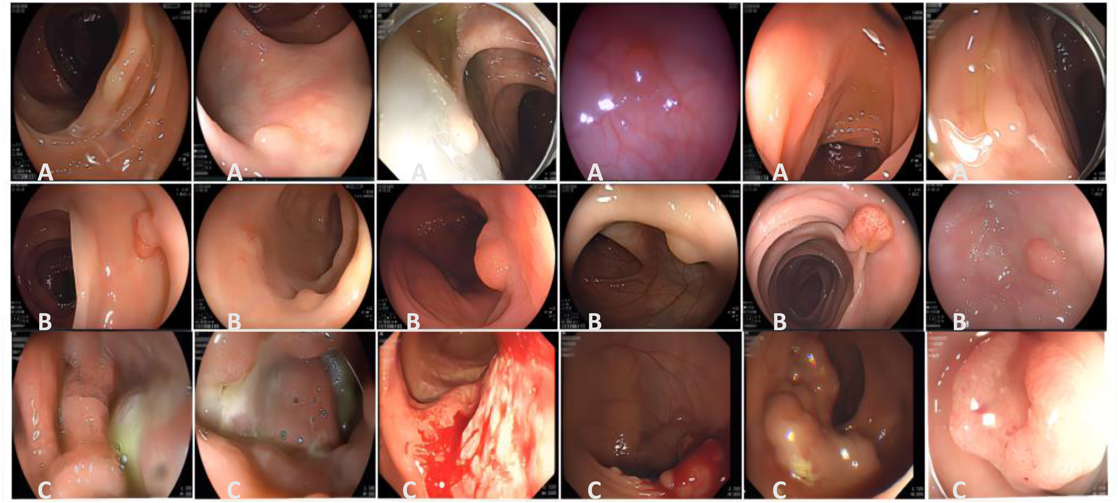
Representative images from the datasets. A1-A6 depict NICE type 1, B1-B6 depict NICE type 2, and C1-C6 depict NICE type 3.

This study excluded patients under the following circumstances: inflammatory bowel disease, active colitis, coagulation dysfunction, familial polyposis, emergency colonoscopy, and those with incomplete diagnostic or therapeutic information. Figure 2(a) depicts the distribution of all image dimensions across the three datasets. Herein, the color yellow signifies a concentration of homologous image quantities at that dimension, while purple denotes a lesser quantity. This clearly showcases a multitude of image dimensions encompassed within the datasets, with dimensions 1280 × 995 and 1504 × 1080 being particularly prevalent. Figure 2(b) illustrates the composition and distribution of lesion types across the training set, test set, and external test set.

Figure 2.

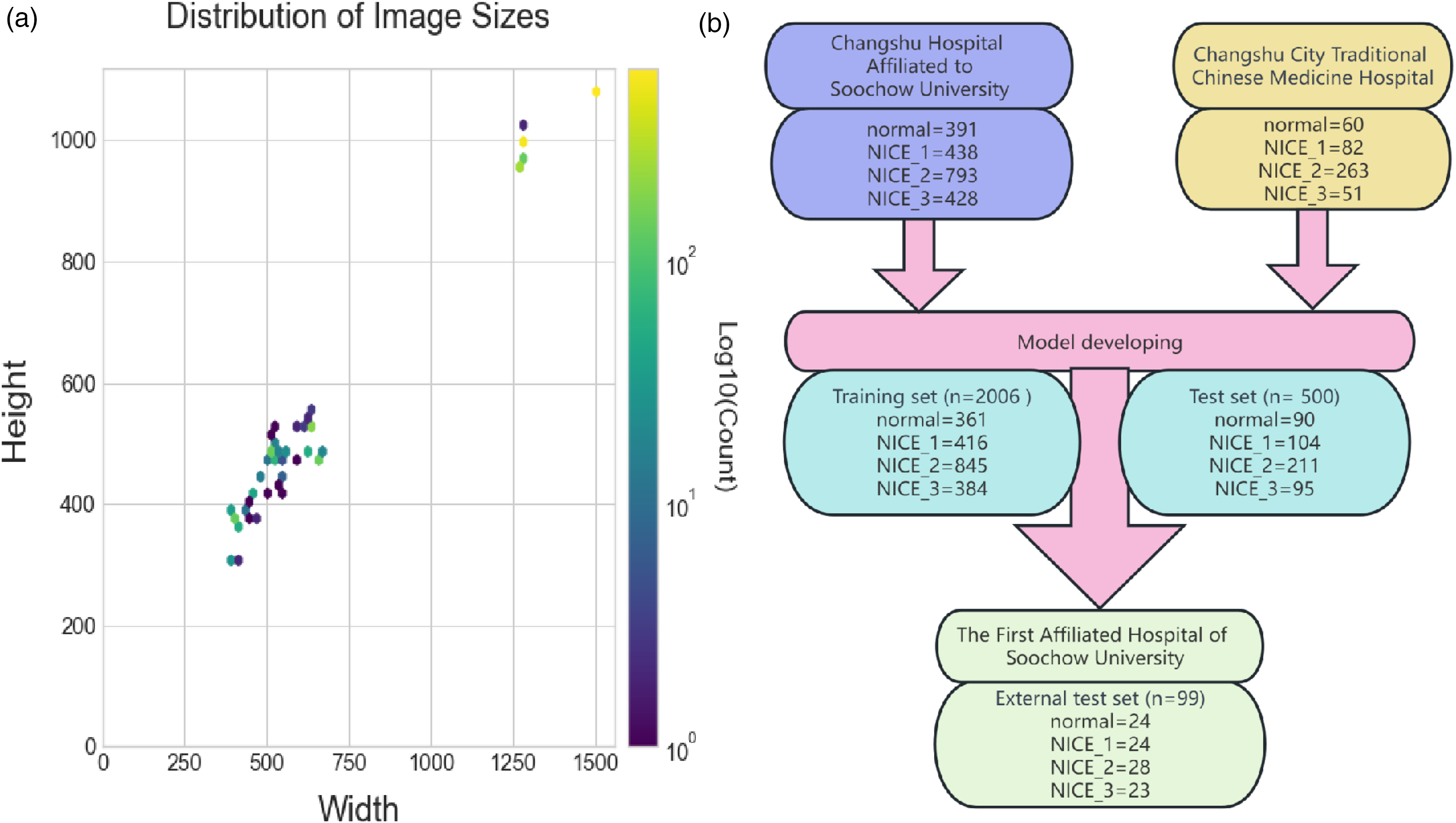
(a) Distribution of image sizes in the dataset. (b) Distribution of images across different categories.

Image labelling

In this study, all lesions discovered during colonoscopic examinations were excised and subjected to histopathological analysis. The pathological findings were documented within the electronic medical records system. We incorporated 2605 colonoscopic images, wherein aside from those categorized as “normal”, all images were pathologically validated. In instances where biopsy and excised specimen pathological results were present, the latter was deemed authoritative. To assure image integrity, we employed meticulously maintained high-resolution endoscopes, and executed stringent intestinal preparation for each patient. Within the pathological diagnostic results were: 475 normal cases, 544 instances of inflammatory hyperplasia, 1084 cases of adenomas/mucosal carcinoma, and 502 instances of infiltrative carcinoma.

The NICE classification, proposed by Tanaka et al. in 2011,¹⁶ primarily evaluates the infiltration depth of tumors through the observation of the lesion's surface structure, vasculature, and color. This typology does not necessitate magnified endoscopy, rendering it straightforward and highly amenable for utilization by junior physicians and for clinical propagation. The NICE classification delineates lesions into three categories based on color, microvascular structure, and surface characteristics: Type 1 represents proliferative polyps; Type 2 signifies neoplastic alterations, encompassing adenomas, mucosal carcinoma (M), and superficial submucosal infiltrative carcinoma (SM1); whereas Type 3 denotes tumors with deep submucosal infiltration (SM2) or deeper. In accordance with the pathological findings of the incorporated images, and when juxtaposed with the NICE classification, the following was deduced: 544 images were of NICE Type 1, 1084 images of NICE Type 2, and 502 images of NICE Type 3.

Deep learning networks

Image preprocessing

To enhance the model's generalization capability, we applied real-time (online) data augmentation during training,¹⁷ ensuring the model encountered slightly varied versions of the same image in each epoch. For the training set, input images were randomly resized and cropped to 224 × 224, followed by random horizontal flipping. Additionally, we introduced brightness variation and noise perturbation to simulate realistic image degradation and improve the model's robustness under suboptimal imaging conditions. Images were then converted to PyTorch tensors and normalized to the [0, 1] range, and standardized using channel-wise z-score normalization with ImageNet mean values [0.485, 0.456, 0.406] and standard deviations [0.229, 0.224, 0.225]. For the test set, the short edge was resized to 256 pixels and then center-cropped to 224 × 224. The remaining normalization and standardization steps were identical to those used for the training set. All preprocessing operations were performed using the torchvision library.

Model training configuration

For the image classification task, we employed transfer learning using CNN- and Transformer-based models pretrained on the ImageNet dataset. Within the CNN realm, EfficientNet,¹⁸ ResNet50,¹⁹ and VGG19²⁰ models were selected; whereas within the Transformer realm, ViT,²¹ Swin,²² and CvT²³ models were chosen. The pretrained weights for CNNs were obtained via the torchvision.models library, while Transformer-based models were initialized using weights from the timm (PyTorch Image Models) repository, available at https://github.com/huggingface/pytorch-image-models. All models were fine-tuned on our dataset through transfer learning. The corresponding neural network architectures are illustrated in Supplementary Figure 1.

The CNN models consist of convolutional layers, average pooling layers, and fully connected layers with ReLU activation. To better adapt to our dataset, two additional dense layers with ReLU activation and a final output layer with Softmax activation were appended to each pre-trained model. The output layer was configured to have 4 neurons, corresponding to our 4-class classification task. During training, cross-entropy was used as the loss function. For EfficientNet and ResNet50, Adam was employed as the optimizer with an initial learning rate of 1e⁻⁴ and no weight decay, while VGG19 used SGD with a momentum of 0.9 and an initial learning rate of 1e⁻³. The learning rate was reduced by half every 5 epochs, and training lasted for 35 epochs with a batch size of 60. An early stopping mechanism with a patience of 8 epochs was applied to prevent overfitting. The training hyperparameter settings are detailed in Table 1.

Table 1.

Training hyperparameters for different models.

Model	Learning Rate	Optimizer	Learning Rate Scheduler	Batch Size	Weight Decay	Epochs	Patience
EfficientNet	1e⁻⁴	Adam	StepLR	60	0	35	8
ResNet50	1e⁻⁴	Adam	StepLR	60	0	35	8
VGG19	1e⁻³	SGD	StepLR	60	0	35	8
ViT_Base	1e⁻³	Adam	StepLR	32	0	35	8
Convit	1e⁻⁵	AdamW	StepLR	64	1e-4	60	8
Swin	1e⁻⁵	AdamW	StepLR	64	1e-4	60	8

For the Transformer models, random cropping, horizontal flipping, and rotations of up to 15 degrees were applied during image preprocessing. The models included ViT_Base_Patch32_224, Swin_Tiny, and ConViT. ViT and Swin were trained using Adam and AdamW optimizers, respectively, with an initial learning rate of 1e⁻³ for ViT and 1e⁻⁵ for Swin and ConViT, both with a weight decay of 1e⁻⁴. The training hyperparameter settings, including optimizer types, learning rates, and other configurations, are detailed in Table 1. The learning rate scheduler StepLR was set to decrease the learning rate by a factor of 0.1 every 7 epochs. The Transformer models were trained for 60 epochs, with a batch size of 64 for Swin and ConViT, and 32 for ViT. Early stopping was also implemented with a patience of 8 epochs. For classification, the models divided input images into fixed-size patches, encoded positional information, and used Transformer encoders to capture patch-level relationships. Finally, the output of the first patch was utilized for 4-class classification.

To track withdrawal speed during colonoscopy, we utilized perceptual hash functions to measure changes between consecutive video frames. The workflow, built with OpenCV and PyTorch, calculated the perceptual hash (pHash) for each frame using the imagehash library. The hash value was derived as H = pHasH(I), where I denotes the input image. The degree of visual change between frames was quantified by computing the Hamming distance D, defined as D = H1-H2, where H1 and H2 are the hash values of consecutive frames. This metric reflects the magnitude of content variation. To visualize withdrawal speed, a scale indicator was overlaid on each frame, its position determined by the value of D. Color coding was applied: blue for normal speed (D ≤ 20), yellow for warning speed (21 ≤ D ≤ 30), and red for hazardous speed (D > 30).

Model interpretation

Despite the wide application of advanced computer vision technologies in medical imaging, their proliferation within the medical community remains hindered by high computational costs, data constraints, and the black-box nature of deep learning. To enhance transparency, Explainable Artificial Intelligence (XAI) has been introduced, aiming to unveil the internal mechanisms and decision-making processes of deep learning models. To surmount this “black-box effect”, we conducted an in-depth interpretability analysis on high-performance models based on CNN and Transformer, employing techniques such as gradient-weighted class activation mapping (Grad-CAM), guided Grad-CAM, and SHAP.^24–26 Among these, Grad-CAM generates heatmaps to disclose the key image regions in model decision-making; Guided Grad-CAM amalgamates Grad-CAM with Guided Backpropagation, offering a more refined perspective on pixel contributions during the decision process. Concurrently, SHAP allocates significance to each pixel in image classification, elucidating their roles in decision-making. These techniques collectively deepened our understanding of the automated NICE classification of colorectal lesions.

In this investigation, deep learning was employed for the automated NICE categorization of colorectal lesions into normal, NICE Type 1, NICE Type 2, and NICE Type 3. To delineate the model's semantic classification efficacy, intermediate layer outputs from the image classification model were harnessed as semantic features. Utilizing forward hooks registered to the targeted layer, these features were captured. The high-dimensional features were subsequently reduced to a two-dimensional space using the t-SNE method,²⁷ and visualized utilizing the Plotly library.

Deployment of model across multiple devices

To automate the NICE classification of colorectal lesions, a deep learning model was developed and deployed across multiple devices including desktop computers, laptops, and online browsers at endoscopy centers. This model aims for real-time and precise monitoring during colonoscopy examinations, adhering to minimal FPS requirements to encompass the entire process. Leveraging transfer learning, specific optimizations were made to the PyTorch-based model. For seamless cross-platform deployment, the model was converted to the ONNX format, enabling efficient operation across various operating systems (e.g., Linux, Windows, MacOS) and hardware configurations (CPU, GPU) via ONNX Runtime. As an open standard, ONNX not only facilitates model interoperability but expands deployment options, thus enhancing real-time lesion recognition accuracy in colonoscopy videos.²⁸ Refer to Supplementary Figure 2 for the model development and deployment workflow.

Experimental platform and evaluation metrics

In this investigation, a computer outfitted with an RTX A4000 graphics card (16GB memory), 5×E5-2680 v4 CPUs, and 350GB disk space was utilized. Employing Python libraries including TensorFlow (2.7.0), Keras (2.7.0), and OpenCV (4.5.4.60), we efficiently built and trained deep learning models, and processed images. Data organization, analysis, and visualization were facilitated through Pandas (1.3.4), NumPy (1.21.4), Matplotlib (3.5.0), and Plotly (5.4.0). Model optimization was executed using PyTorch (1.10.0 + cu113), while model saving and loading were handled by H5py (3.6.0). To ascertain model robustness and broad applicability, an exhaustive evaluation on an independent test set was conducted. The principal evaluation metrics entailed the accuracy of internal and external testing. Additional performance metrics, including precision or positive predictive value (defined as [true positives/true positives + false positives]), recall or sensitivity (defined as [true positives/true positives + false negatives]), and F1 score (2 × precision × recall/precision + recall) were meticulously calculated. Through the ROC curve and its AUC value, model performance at varying thresholds was assessed. Specifically, predictions with confidence levels of 80% or above were deemed highly confident, indicative of reliable model predictions. Given the retrospective design and image anonymization, the requirement for written informed patient consent was waived.¹³

Results

Clinical class distributions of datasets

During the study period, 2248 colorectal lesions from 1835 patients were examined. The cohort comprised 993 males and 842 females, with an average age of 59 ± 25.3 years. Pathological assessments revealed 575 cases of hyperplasia (25.6% of total), 1143 instances of adenomas/mucosal in-situ carcinomas, and 530 cases of invasive carcinomas. Among them, 1027 (45.69%) were identified as adenomas, with a median size of 6.3 mm (range: 2–25 mm). Refer to Table 2 for detailed characteristics of the colorectal lesions.

Table 2.

Characteristics of colorectal lesions.

Variables	Overall set (n = 2248)
Histological type
hyperplasia	575.0 (25.6%)
adenomas/mucosal in-situ carcinomas	1143.0 (50.84%)
invasive carcinomas	530.0 (23.58%)
Size(in mm)
≤5 mm	643.0 (28.6%)
6 mm to <10 mm	933 (41.5%)
≥10 mm	672.0 (29.9%)
Location
Rectum-sigma	513.0 (22.8%)
Others	1735.0 (77.2%)

Comparative analysis of deep learning models for automated NICE classification

We evaluated six deep learning models—three CNN-based and three Transformer-based—on a test set of 500 colonoscopy images. As shown in Table 3, EfficientNet outperformed the other models, achieving the highest accuracy (0.910), precision (0.918), recall (0.914), and F1 score (0.916), demonstrating strong robustness and classification effectiveness. ResNet50 and VGG19 followed with accuracies of 0.884 and 0.868, respectively. While Transformer models generally underperformed compared to CNNs, ViT showed the best performance among them, reaching an accuracy of 0.664, indicating potential for improvement with further optimization. The training process of EfficientNet also showed stable convergence, with a final test loss of 0.303 after 30 epochs. Supplementary Figures 3 and 4 present the training curves of loss, accuracy, precision, recall, and F1 score, providing insight into the model's learning dynamics and overall consistency.

Table 3.

Performance metrics of different models.

Architecture	Model	Accuracy	Precision	Recall	F1-score	FPS
CNN	EfficientNet	0.910	0.918	0.914	0.916	121
	resnet50	0.884	0.893	0.890	0.891	152
	VGG19	0.868	0.876	0.867	0.869	94
Transformer	vit_base	0.664	0.686	0.637	0.648	76
	CvT	0.656	0.687	0.615	0.635	98
	Swin	0.592	0.478	0.521	0.481	57

Model predictive performance on external test set

We developed the EfficientNet deep learning model for automated NICE classification of colorectal lesions using a dataset (n = 2506) from the Affiliated Changshu Hospital of Soochow University and Changshu Traditional Chinese Medicine Hospital. To evaluate the model's generalizability, we employed 99 colonoscopy images from the First Affiliated Hospital of Soochow University as an external test set. This independent validation helps assess the model's real-world performance and mitigates overfitting concerns.

On the external test set, the EfficientNet model demonstrated outstanding classification. AUC values for NICE Type 1 and Type 2 were 0.988 and 0.989, respectively, highlighting its discriminative prowess. The AUC for NICE Type 3 reached 0.995 (Figure 3(a)). Overall, the model achieved a macro-average precision of 0.9360, recall of 0.9177, and AUC of 0.9943, with weighted metrics at 0.9296, 0.9192, and 0.9940.

Figure 3.

Predictive performance of the model on the external test set. (a) Receiver operating characteristic (ROC) curve; (b) Precision-recall (PR) curve.

As shown in Figure 3(b)'s PR curve, the model exhibited a precision of 0.950 and recall of 0.792 for NICE Type 1, closely approaching optimal levels. For NICE Type 2, precision was 0.794 with a notable recall of 0.964. NICE Type 3 delivered a precision of 1.00 and recall of 0.957. Despite slight recall variations in some categories, each category's average precision (AP) surpassed 0.970, underscoring the model's robustness. A confusion matrix, presented in Figure 4(a), further confirmed its classification efficacy across categories.

Figure 4.

Model performance on the external test set. (a) Confusion matrix. (b) Image example with true label as NICE 1, but predicted by the model as NICE 2. (c) Image example with true label as normal, but predicted by the model as NICE 2. (d) Image example with true label as NICE 2, but predicted by the model as NICE 1.

In our research, the DL model largely demonstrated consistent accuracy, but certain misclassifications were observed. Figure 4 highlights these: Figure 4(b) depicts NICE 1 images classified as NICE 2; Figure 4(c) shows a ‘normal’ image predicted as NICE 2; and Figure 4(d) presents a NICE 2 image identified as NICE 1. Factors such as overlapping image features, unintended reflections, capture distances, and image blur may have contributed to these errors.

To unveil underlying patterns and enhance our analysis, we employed t-SNE to project high-dimensional image features onto a two-dimensional plane. Supplementary Figure 5 illustrates orange circles (NICE Type 1) overlapping with purple stars (NICE Type 2), implying potential misclassifications. The light green ‘+’ symbols distinctly indicate NICE Type 3. Following a comprehensive review by two physicians, a labeling error was identified. Additionally, we created an interactive three-dimensional semantic feature map using the plotly library, enabling users to intuitively explore the distribution of external test set images (Supplementary Figure 6) by dragging with a finger or mouse for interactive navigation.

Deep learning vs. endoscopists diagnostic performance

In an external dataset of 99 colorectal lesion images, we compared the EfficientNet deep learning model's predictive capacity for NICE classification with that of endoscopists. For NICE Type 1, the model's sensitivity was 0.792, marginally lower than the endoscopists’ 0.823, but its specificity of 0.950 closely matched the endoscopists’ 0.973. For NICE Type 2 predictions, the model achieved a sensitivity of 0.964, exceeding the endoscopists’ 0.893, but lagged in specificity at 0.794 compared to the endoscopists’ 0.965. In NICE Type 3, the model's sensitivity was 0.957, comparable to the endoscopists’ 0.977, but showcased a flawless specificity of 1.000, surpassing the endoscopists’ 0.949. In summary, EfficientNet paralleled endoscopists in certain metrics and excelled in others.

In our research, an 80% confidence threshold was delineated for each NICE classification category pertaining to colorectal lesions, with the aim of appraising the predictive accuracy between endoscopists and the model. Confidence levels meeting or surpassing the 80% threshold are classified as high confidence, whereas those falling below this benchmark are categorized as low confidence. This arrangement endeavors to ensure a substantial degree of reliability across most predictions. As depicted in Figure 5, each circlet symbolizes a colorectal lesion; the green and gray hues denote accurate and erroneous predictions, respectively, while solid and semi-circular icons represent high and low confidence predictions, respectively. This illustration succinctly contrasts the predictive assessments of endoscopists and the EfficientNet model on an external independent testing cohort.

Figure 5.

Diagnostic performance: deep learning model (EfficientNet) vs. endoscopist. Left: EfficientNet predictions. Right: Endoscopist predictions. (a) NICE 1 category. (b) NICE 2 category. (c) NICE 3 category.

Model interpretation

To improve the interpretability of the model's predictions, we applied Grad-CAM, Guided Grad-CAM, and SHAP to visualize the decision basis for NICE classification. As shown in Figure 6, the attention heatmaps generated by Grad-CAM and its guided variant highlighted lesion areas with distinct surface texture, vascular patterns, and color changes—features that align with clinical diagnostic criteria. SHAP analysis (Figure 7) further confirmed that pixel-level contributions were consistent with the histological characteristics of NICE Type 2 and Type 3 lesions. These results suggest that the model relies on clinically meaningful features in its classification process, supporting its reliability for use in AI-assisted optical diagnosis.

Figure 6.

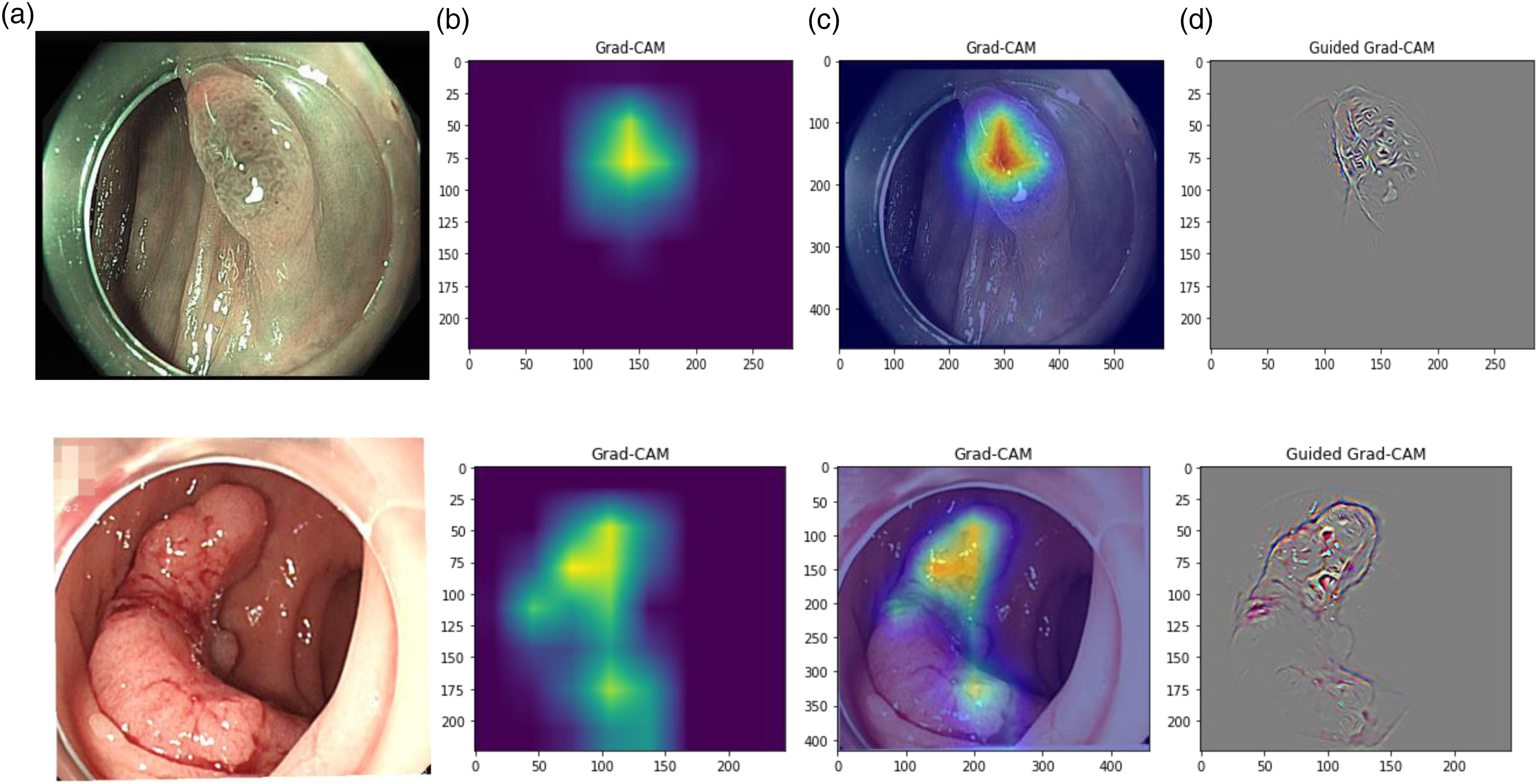
Interpretative analysis of automated NICE classification model. Column a: Original endoscopic image; Column b: Pixel activation heatmap using Grad-CAM; Column c: Composite of original image with activation heatmap; Column d: Fine-grained heatmap via Guided Grad-CAM.

Figure 7.

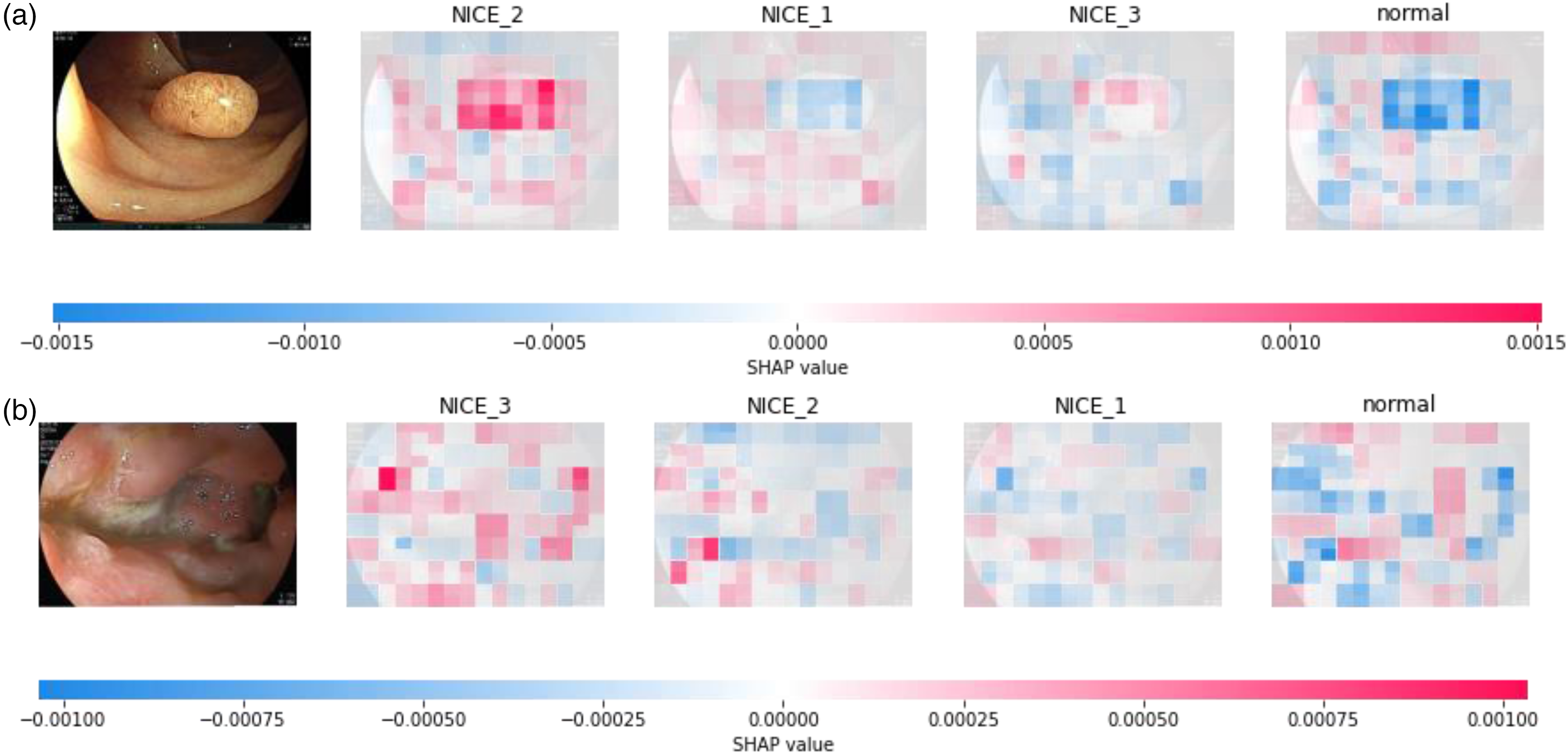
Interpretative analysis via SHAP. (a) SHAP visualization for a correctly predicted label of NICE 2; (b) SHAP visualization for a correctly predicted label of NICE 3.

Model-based video prediction and multi-terminal deployment

We trained the EfficientNet model via transfer learning in PyTorch, converted it to ONNX for standardized cross-platform deployment, and integrated it with OpenCV for real-time NICE classification on both local and web-based systems. Supplementary Figure 7 illustrates a single frame's prediction outcome. The left image showcases the original frame with the top two classifications and their respective confidence levels. while the right displays a confidence bar chart. Subfigures A and B detail predictions for images labeled NICE Type 1 and NICE Type 2. Subfigures C and D, using QR codes, demonstrate real-time video predictions, with C highlighting a local computer deployment and D showing predictions via the computer's camera. Subfigures E illustrates the predictive performance of the AI model, enhanced with colonoscope withdrawal speed monitoring functionality. The current withdrawal speed is displayed in real time on a scale in the lower-left corner of the video screen. If the speed exceeds the safe limit, the scale moves into the red zone, triggering a “dangerous speed” warning. When the speed stays within the acceptable range, a blue “normal speed” indicator appears. Otherwise, a yellow “caution speed” alert is shown.

Discussion

In this study, we crafted six DL-based CV models for the automated NICE classification of colorectal lesions: three employing CNN architectures and three utilizing Transformer frameworks. Drawing upon colonoscopy datasets from three major hospitals in Jiangsu Province, China, we curated 2506 images marked by NICE 1, NICE 2, NICE 3, and conventional colonic features for model development and validation. After evaluation with an external test set, the EfficientNet model stood out as the superior performer. This model has been successfully deployed across multiple platforms for real-time video predictions. The study comparatively evaluates the performance of CNN and Transformer in automated NICE classification, identifying the optimal model and encompassing the entire process from model development and testing to interpretable analysis and multi-terminal deployment.

Advanced endoscopic methods, such as confocal laser, traditional staining, and magnifying endoscopy, confront technical and cost barriers. Deep learning has showcased its efficacy in medical imaging, notably in gastroenterological endoscopic diagnosis.²⁹ Recent AI research in gastroenterology has delved into the prospects of AI-enhanced medical solutions. Our NICE automatic classification model, utilizing the ONNX format, enhances cross-framework interoperability. The EfficientNet model, deployed on platforms like local computers and web interfaces, achieves over 50 FPS during colonoscopies, ensuring timely and precise lesion categorization. This model presents an efficient NICE classification alternative for budget-restricted endoscopy centers. Furthermore, the withdrawal speed monitoring module was designed in accordance with ASGE guidelines,³⁰ which emphasize the withdrawal phase as a key quality control indicator during colonoscopy. Our perceptual hash–based system effectively captures image instability from either fast withdrawal or abrupt motion, thus providing timely alerts to endoscopists to maintain a steady and safe withdrawal technique.

Optical diagnostic methods discern the tumorous characteristics of polyps. Given that a majority of polyps found in colonoscopies measure ≤5 mm with minimal histological risk, optical diagnosis emerges as a cost-effective and safer alternative to histopathological evaluation.³¹ Recognizing its cost-efficiency, esteemed bodies like ASGE, BSG, and ESGE have endorsed the “resect and discard” approach,^32–34 contingent on a ≥ 90% agreement between optical and histopathological diagnoses. Aligning with this, our EfficientNet model achieved 91.03% accuracy on a standard dataset and escalated to 91.92% on an external set, highlighting its reliability. This consistent performance suggests the model's potential to bolster the “resect and discard” strategy when combined with optical diagnostics.

The NICE classification, introduced by CTNIG in 2009, serves as the international standard for colorectal NBI imagery, distinguishing colorectal lesions. It categorizes lesions into three types: hyperplastic polyps (NICE 1), adenomatous polyps and early carcinomas (NICE 2), and deeply invasive cancers (NICE 3). This classification offers clinical guidance for colorectal lesion decisions, such as resection strategies or surgical techniques. Recently, Y. Hamada et al. (2021)⁹ and Wang et al. (2021)³⁵ evaluated the application of NICE classification in colorectal lesion diagnosis. Hamada's team reported sensitivities of 86.0%, 99.2%, and 81.8% for NICE types 1, 2, and 3, respectively, with corresponding specificities of 99.6%, 85.2%, and 99.6%, and accuracies of 98.5%, 97.8%, and 99.3%. Wang's study contrasted the diagnostic capabilities of high-experience versus low-experience endoscopists, revealing sensitivities of 84.6%, 91.4%, and 91.7% for the high-experience group and 82.1%, 89.8%, and 83.3% for the low-experience group. Compared to these studies, our model exhibited commendable sensitivity for NICE 1 and NICE 2, though the sensitivity for NICE 2 was slightly lower at 96.4% versus Hamada's 99.2%. For NICE 3, our model achieved a sensitivity of 95.65%, surpassing Hamada's 81.8%. Overall, our EfficientNet model demonstrated comparable or superior performance across NICE categories relative to other studies.

In our study, CNN models notably outperformed Transformer models in the NICE automatic classification of colorectal lesions. While Transformers, such as ViT, have excelled in various NLP and image tasks,^36,37 traditional CNNs like EfficientNet surpassed them in key metrics like Accuracy, Precision, Recall, and F1-Score. This can be attributed to CNNs’ proficiency, especially EfficientNet's, in capturing image local structures and spatial hierarchies, which are essential for colonoscopic image classification.^38,39 Based on this perspective, Zhou T et al.⁴⁰ proposed a novel approach using a Volume Memory Network (VMN) for interactive segmentation of 3D medical images, effectively leveraging the spatial advantages inherent in 3D data. Experiments on three public datasets demonstrated outstanding performance. While our study focuses on the NICE classification task for 2D endoscopic images, the success of this method indicates that, in suitable scenarios, incorporating 3D data and its spatial information could further enhance classification performance. On the other hand, Transformers, particularly ViT, often require vast training data to maximize their capabilities.⁴¹ In data-limited scenarios, EfficientNet may better resist overfitting, leading to enhanced test dataset performance.⁴²

In our study, we compared the EfficientNet deep learning model's predictive capabilities in NICE classification of colorectal lesions with those of endoscopists. While the model's sensitivity for NICE 1 was slightly lower than the physicians’, its specificity was comparable. For NICE 2 and NICE 3, the model occasionally outperformed the physicians, notably achieving perfect specificity for NICE 3. This suggests that deep learning might offer enhanced discriminative power in certain colorectal lesion classifications. The learning curve represents skill or knowledge acquisition rate.⁴³ Zhuo, Lu, and Sun (2021) identified that novice physicians needed to observe 900 colonic polyp images to stabilize in NICE classification under non-magnifying endoscopy.⁴⁴ The EfficientNet model developed in this study could help accelerate this learning process in several ways. First, it provides real-time NICE classification with confidence scores during colonoscopy, enabling immediate feedback for trainees. Second, using Grad-CAM and SHAP, the model highlights key lesion areas that inform its decisions, allowing learners to better understand the visual features associated with each NICE type. These functions together support faster recognition, reinforce diagnostic reasoning, and ultimately shorten the learning curve for endoscopists.

We explored the interpretability of the EfficientNet model using techniques like Grad-CAM, Guided Grad-CAM, and SHAP. While deep learning models are often termed “black boxes”, our use of the torchcam library and Grad-CAM enabled visualization of key decision regions for colorectal lesion NICE classification. EfficientNet's activation heatmaps revealed the model's focal points. Guided Grad-CAM further delineated these regions, and SHAP assessed the contribution of individual pixels to predictions. Using Grad-CAM as an example, we observed that the regions highlighted by the model were highly correlated with key features driving classification decisions, such as surface texture, vascular patterns, and color variations. These features align closely with the NICE classification criteria. This analysis not only enriched our understanding of the model but also provided a nuanced view into its decision-making process.

This study has several notable limitations. First, the dataset used primarily consisted of high-quality colonoscopic images with adequate bowel preparation, which may limit the model's applicability in more complex clinical scenarios, such as poor lighting, motion blur, or inadequate bowel cleanliness. Second, although the model demonstrated good generalizability on an independent external test set, further large-scale, multi-center validation in more diverse patient populations is needed to enhance its clinical utility. Third, during dataset construction, we intentionally excluded certain clinical conditions—such as inflammatory bowel disease, active colitis, and cases with incomplete diagnostic information—to ensure labeling accuracy and improve training stability. While this strategy facilitated model convergence, it may have reduced the dataset's representativeness of real-world clinical complexity. Lastly, future studies should incorporate more diverse and unfiltered clinical images to comprehensively evaluate and improve the model's generalizability in real-world settings.

Conclusion

Our study encompassed the full spectrum from model development to multi-terminal deployment, resulting in a tailored EfficientNet model for automatic NICE classification of colorectal lesions. With a 91.92% accuracy on an independent test set, the model outperformed existing research and excelled in NICE 2 and NICE 3 classifications compared to endoscopists. Given the criticality of early colorectal cancer detection, this model provides robust support for clinical decisions, potentially accelerating novice endoscopists’ proficiency in NICE classification and enhancing patient care.

Supplemental Material

sj-docx-1-dhj-10.1177_20552076251393296 - Supplemental material for Real-time deep-learning NICE classification and withdrawal-speed monitoring for colorectal endoscopy

Supplemental material, sj-docx-1-dhj-10.1177_20552076251393296 for Real-time deep-learning NICE classification and withdrawal-speed monitoring for colorectal endoscopy by Ganhong Wang, Limei Yin, Zhijia Shen, Kaijian Xia, Xiaodan Xu and Jian Chen in DIGITAL HEALTH

Footnotes

ORCID iDs

Ganhong Wang

Xiaodan Xu

Jian Chen

Ethics approval and consent to participate

This study has been approved by the Ethics Review Committee of Changshu Hospital Affiliated to Soochow University (the IRB approval number L2023039). This study was performed in accordance with the Declaration of Helsinki, and written informed consent was obtained from all participants.

Author contribution

Author contributions WGH and YLM contributed equally to this work.

WGH and CJ worked on the study design. YLM and SZJ worked on data collection. CJ and XKJ worked on data analysis. WGH worked on manuscript preparation. XXD and XKJ provided administrative, technical, or material support. XXD supervised the study. All authors have made a significant contribution to this study and have approved the final manuscript.

Funding

The authors disclosed receipt of the following financial support for the research, authorship, and/or publication of this article: Changshu City Science and Technology Plan Project (CS202452); Suzhou Health Information and Medical Big Data Society Project (SZMIA2402); Health Informatics Key Support Discipline Funding of Suzhou City (SZFCXK202147); Suzhou City's 23rd Science and Technology Development Plan Project (SLT2023006); Suzhou Science and Technology Key Project (SYW2025034); Jiangsu Province Traditional Chinese Medicine Science and Technology Development Program Project (MS2024084); No funding body had any role in the design of the study and collection, analysis, interpretation of data, or in writing the manuscript.

Declaration of Conflicting Interests

The authors declared no potential conflicts of interest with respect to the research, authorship, and/or publication of this article.

Data availability

The datasets analysed during the current study are available from the corresponding author on reasonable request.

Supplemental material

Supplemental material for this article is available online.

References

Vuik

Nieuwenburg

Bardou

, et al. Increasing incidence of colorectal cancer in young adults in Europe over the last 25 years. Gut 2019; 68: 1820–1826.

Yin

Lin

Liu

, et al. Development of a deep learning model for malignant small bowel tumors survival: a SEER-based study. Diagnostics 2022; 12: 1247.

Hoffman

Sar

Goetz

, et al. High definition colonoscopy combined with i-scan is superior in the detection of colorectal neoplasias compared with standard video colonoscopy: a prospective randomized controlled trial. Endoscopy 2010; 42: 827–833.

Chan

SCH

Liang

. Advances in tests for colorectal cancer screening and diagnosis. Expert Rev Mol Diagn 2022; 22: 449–460.

Montminy

Jang

Conner

, et al. Screening for colorectal cancer. Med Clin North Am 2020; 104: 1023–1036.

Lim

Nistala

KRY

, et al. Endoscopic submucosal dissection vs endoscopic mucosal resection for colorectal polyps: a meta-analysis and meta-regression with single arm analysis. World J Gastroentero 2021; 27: 3925–3939.

Quero

Fiorillo

Longo

, et al. Propensity score-matched comparison of short- and long-term outcomes between surgery and endoscopic submucosal dissection (ESD) for intestinal type early gastric cancer (EGC) of the middle and lower third of the stomach: a European tertiary referral center experience. Surg Endosc 2021; 35: 2592–2600.

Yeh

Huang

Lee

, et al. Long-term outcomes of endoscopic submucosal dissection and comparison to surgery for superficial esophageal squamous cancer: a systematic review and meta-analysis. Therap Adv Gastroenterol 2020; 13: 320814116.

Hamada

Tanaka

Katsurahara

, et al. Utility of the narrow-band imaging international colorectal endoscopic classification for optical diagnosis of colorectal polyp histology in clinical practice: a retrospective study. BMC Gastroenterol 2021; 21: 336.

10.

Repici

Ciscato

Correale

, et al. Narrow-band imaging international colorectal endoscopic classification to predict polyp histology: REDEFINE study (with videos). Gastrointest Endosc 2016; 84: 479–486.

11.

Yousefzadeh

Hasanpour

Zolghadri

, et al. Deep learning framework for prediction of infection severity of COVID-19. Front Med-Lausanne 2022; 9: 940960.

12.

Chen

Xia

Zhang

, et al. Establishing an AI model and application for automated capsule endoscopy recognition based on convolutional neural networks (with video). BMC Gastroenterol 2024; 24: 394.

13.

Gong

Bang

Lee

, et al. No-code platform-based deep-learning models for prediction of colorectal polyp histology from white-light endoscopy images: development and performance verification. J Pers Med 2022; 12: 963.

14.

Garcia-Rodriguez

Tudela

Cordova

, et al. In vivo computer-aided diagnosis of colorectal polyps using white light endoscopy. Endosc Int Open 2022; 10: E1201–E1207.

15.

Wang

Liu

Glissen Brown

, et al. Lower adenoma miss rate of computer-aided detection-assisted colonoscopy vs routine white-light colonoscopy in a prospective tandem study. Gastroenterology 2020; 159: 1252–1261.

16.

Tanaka

Sano

. Aim to unify the narrow band imaging (NBI) magnifying classification for colorectal tumors: current status in Japan from a summary of the consensus symposium in the 79th annual meeting of the Japan gastroenterological endoscopy society. Dig Endosc 2011; 23: 131–139.

17.

Athalye

Arnaout

. Domain-guided data augmentation for deep learning on medical imaging. PLOS one 2023; 18: e282532.

18.

Chen

Zhu

Papandreou

, et al. Encoder-decoder with atrous separable convolution for semantic image segmentation. In: Conference Paper ‘Paper presented at‘ Computer Vision – ECCV 2018, 2018.

19.

Zhang

Ren

, et al. Deep residual learning for image recognition. In: Conference Paper ‘Paper presented, Las Vegas, NV, USA, 2016.

20.

Bansal

Kumar

Sachdeva

, et al. Transfer learning for image classification using VGG19: caltech-101 image data set. J Amb Intel Hum Comp 2023; 14: 3609–3620.

21.

Yao

Pan

, et al. Dual vision transformer. IEEE T Pattern Anal 2023; 45: 10870–10882.

22.

Liu

Lin

Cao

, et al. Swin transformer: Hierarchical vision transformer using shifted windows. In: Conference Paper ‘Paper presented, Montreal, QC, Canada, 2021.

23.

Xiao

Codella

, et al. CvT: Introducing convolutions to vision transformers. In: Conference Paper ‘Paper presented at‘ 2021 IEEE/CVF International Conference on Computer Vision (ICCV), Montreal, QC, Canada, 2021.

24.

Zhang

Hong

McClement

, et al. Grad-CAM helps interpret the deep learning models trained to classify multiple sclerosis types using clinical brain magnetic resonance imaging. J Neurosci Meth 2021; 353: 109098.

25.

Kikutsuji

Mori

Okazaki

, et al. Explaining reaction coordinates of alanine dipeptide isomerization obtained from deep neural networks using explainable artificial intelligence (XAI). J Chem Phys 2022; 156: 154108.

26.

Zhang

. Genomic pan-cancer classification using image-based deep learning. Comput Struct Biotec 2021; 19: 835–846.

27.

Linderman

Steinerberger

. Clustering with t-SNE, provably. Siam J Math Data Sci 2019; 1: 313–332.

28.

Wang

Huang

, et al. Multi-model running latency optimization in an edge computing paradigm. Sensors (Basel, Switzerland) 2022; 22(16): 6097.

29.

Guimarães

Keller

Fehlmann

, et al. Deep-learning based detection of gastric precancerous conditions. Gut 2020; 69: 4–6.

30.

Rex

Anderson

Butterly

, et al. Quality indicators for colonoscopy. Gastrointest Endosc 2024; 100: 352–381.

31.

Huynh

, et al. Utility of narrow-band imaging with or without dual focus magnification in neoplastic prediction of small colorectal polyps: a Vietnamese experience. Clin Endosc 2023; 56: 479–489.

32.

Bisschops

East

Hassan

, et al. Advanced imaging for detection and differentiation of colorectal neoplasia: European society of gastrointestinal endoscopy (ESGE) guideline - update 2019. Endoscopy 2019; 51: 1155–1179.

33.

Rutter

East

Rees

, et al. British Society of gastroenterology/association of coloproctology of Great Britain and Ireland/public health England post-polypectomy and post-colorectal cancer resection surveillance guidelines. Gut 2020; 69: 201–223.

34.

East

Vleugels

Roelandt

, et al. Advanced endoscopic imaging: European society of gastrointestinal endoscopy (ESGE) technology review. Endoscopy 2016; 48: 1029–1045.

35.

Wang

, et al. Diagnostic performance of narrow-band imaging international colorectal endoscopic and Japanese narrow-band imaging expert team classification systems for colorectal cancer and precancerous lesions. World J Gastro Oncol 2021; 13: 58–68.

36.

Sun

Qin

Deng

, et al. Vicinity vision transformer. IEEE T Pattern Anal 2023; 45: 12635–12649.

37.

Liu

Zhang

Wang

, et al. A survey of visual transformers. IEEE T Neur Net Lear 2024; 35(6): 7478–7498.

38.

Gao

Yang

Zhang

. Combine EfficientNet and CNN for 3D model classification. Math Biosci Eng 2023; 20: 9062–9079.

39.

Huang

Wang

Zhang

, et al. Tuberculosis diagnosis using deep transferred EfficientNet. IEEE/ACM Trans Comput Biol Bioinf 2023; 20(5): 2639–2646.

40.

Zhou

Bredell

, et al. Volumetric memory network for interactive medical image segmentation. Med Image Anal 2023; 83: 102599.

41.

Zhang

. FV-ViT: vision transformer for finger vein recognition. IEEE Access 2023; 11: 75451–75461.

42.

, et al. A robust approach for brain tumor detection in magnetic resonance images using finetuned EfficientNet. IEEE Access 2022; 10: 65426–65438.

43.

Gkionis

Flamourakis

Tsagkataki

, et al. Multidimensional analysis of the learning curve for laparoscopic colorectal surgery in a regional hospital: the implementation of a standardized surgical procedure counterbalances the lack of experience. BMC Surg 2020; 20: 308.

44.

Zhuo

Sun

. IDDF2021-ABS-0082 Application and learning curve of nice classification for colorectal polyps under non-magnifying endoscopy. Gut 2021; 70: A111.

Supplementary Material

Please find the following supplemental material available below.

For Open Access articles published under a Creative Commons License, all supplemental material carries the same license as the article it is associated with.

For non-Open Access articles published, all supplemental material carries a non-exclusive license, and permission requests for re-use of supplemental material or any part of supplemental material shall be sent directly to the copyright owner as specified in the copyright notice associated with the article.

0.00 MB

2.24 MB