Enhanced MRI-based brain tumor segmentation and feature extraction using Berkeley wavelet transform and ETCCNN

Abstract

Objective

Brain tumors are abnormal growths of brain cells that are typically diagnosed via magnetic resonance imaging (MRI), which helps to discriminate between malignant and benign tumors. Using MRI image analysis, tumor sites have been identified and classified into four distinct tumor categories: meningioma, glioma, not tumor, and pituitary. If a brain tumor is not detected in its early stages, it could progress to a severe level or cause death. Therefore, to address these issues, the proposed approach uses an efficient classifier based on deep learning for brain tumor detection.

Methods

This article describes the classification and detection of brain tumor by an efficient two-channel convolutional neural network. The input image is initially rotated during the augmentation stage. Morphological operations, thresholding, and region filling are then used in the pre-processing stage. The output is then segmented using the Berkeley Wavelet Transform. A two-channel convolutional neural network is used to extract features from segmented objects. In the end, the most effective deep neural network is employed to determine the features of brain tumors. The classifier will utilize the Enhanced Serval Optimization Algorithm to determine the optimal gain parameters. MATLAB serves as the platform of choice for implementing the suggested model.

Results

Several performance metrics are calculated to assess the proposed brain tumor detection method, such as accuracy, F measures, kappa, precision, sensitivity, and specificity. The proposed model has a 98.8% detection accuracy for brain tumors.

Conclusion

The evaluation shows that the suggested strategy has produced the best results.

Introduction

Brain regulates the whole human body's functions and serves as the central nervous system's controller. ¹ Brain tumors are defined as uncontrollably growing and deforming brain tissue. ² Human life is directly at stake from brain tumors. If the tumor is found early, the patient's likelihood of survival is higher. Brain tumors represent a major threat to a patient's life and are a prevalent form of cancer that affects many people globally. ³ Signs and symptoms of brain tumors vary depending on their shape, size, and location. Headaches, nausea, speech changes, vision problems, numbness in extremities, seizures, memory loss, mood changes, behavioral changes, balance problems, and difficulty walking are symptoms. The exact cause of brain tumors is still being investigated. ⁴

Brain tumors are classified into two categories: primary brain tumors and metastatic brain tumors. A brain tumor that first appears there and is known as a primary brain tumor because it often remains there until it spreads. ⁵ Furthermore, Benign brain tumors can be distinguished from, meaning they are not cancerous, or malignant, meaning they include cancerous cells and present a greater risk to life. Accurate identification and categorization of these complicated conditions are essential for providing effective treatment for brain tumors. ⁶

In the last few decades, practitioners have started utilizing cutting-edge methods to find tumors that bring patients greater agony. ⁷ Doctors utilize MRI or CT scanning to detect tumors. A magnetic particle and weak radio wave are used in MRI to produce precise images of the brain's inside. Because MRI can detect even the slightest abnormalities in the brain, neurosurgeons favor it. ⁸ Furthermore, it is among the most useful methods currently in use for identifying advanced-stage brain cancers. ⁹

Conversely, brain cancers can be identified early and without the need for human intervention according to the Computer-Aided Diagnosis technique. CAD systems have the ability to provide diagnostic reports and offer radiologists guidance based on MRI images. In medical imaging, CAD method was enhanced by machine and deep learning techniques. ¹⁰

Type and presence of brain tumors are determined by Machine learning techniques; however, since machine learning models are predictive, additional human intervention is required. However, using neural networks, deep learning models are able to learn and analyze their own features.. ¹¹ Their ultimate goal is to integrate the entire search process is done on a single machine. Based on DL's performances, we aim to investigate the possibility of creating a technique that will aid in brain tumor identification and categorization. ¹² Deep learning is an extremely useful technique for resolving image processing issues in medicine, such as brain tumor identification, tibial cartilage segmentation, and lung cancer diagnosis. ¹³ In medical imaging, CNN is the most widely used deep learning tool. CNN model achieves high performance capabilities and can extract structured and representative information from medical images. ¹⁴ After analyzing the optimizers, we will choose the best one to get the best outcome and utilize it to construct our ultimate sequential model. ¹⁵

Recent developments in computational methods and medical imaging have greatly aided in the early identification and diagnosis of brain cancers. To improve tumor segmentation and classification using medical imaging data, a variety of computational techniques have been used. An overview of some popular models and methods in this field is given in this section. These include Hybrid Approaches (Feature Fusion and Ensemble Methods), Deep Learning Approaches (CNN, U-Net, and Fully Convolutional Networks (FCNs)), and Machine Learning Approaches (Support Vector Machines (SVM), Random Forests, and K-Nearest Neighbors (KNN)). In summary, the use of these computational techniques in brain tumor analysis can greatly improve both treatment planning and diagnostic capacities.

Detection and classification of brain tumors require these details. Numerous investigations have examined the etiology of brain tumors, however, the findings have not proven definitive. Numerous neural network techniques have been employed in less accurate tumor categorization and detection. The segmentation and detection algorithms employed determine the accuracy of the detection. As of right now, the accuracy and image quality of the existing method are less. Because deep learning networks can effectively recognize patterns suggestive of diseases and process enormous volumes of complicated data, ¹⁶ including medical pictures, efficiently, they have become increasingly popular in the field of medical diagnosis. Many deep learning-based models have been investigated recently ¹⁷ for the purpose of detecting brain tumors. Because of its remarkable performance and adaptability, the Convolutional Neural Network (CNN) architecture has been the most widely used of these models.^18,19 The CNN model uses a number of training layers to carry out feature extraction and classification; these layers can be adjusted based on the final performance. To address this issue of detect and categorize brain tumors, we are using an Effective Two Channel Convolutional Neural Network.

An overview of the primary findings of the research is provided below:

ODNN classifier presented in this work is intended to identify brain tumors. The open-source system is where the database is gathered. There will be five stages in the suggested process.

In the Augmentation approach, rotation has been used. To preprocess the augmented output images, employ thresholding, morphological operation, and region filling.

The preprocessed output images are segmented to extract the brain tumor section using Berkeley's Wavelet Transformation (BWT). A two-channel CNN is used to extract features.

Finally, tumor portion will be identified using the ODNN classifier and Enhanced Several Optimization Algorithm will be developed for selecting optimal gain parameters.

Literature review

This section discusses the major studies for diagnosing various brain tumors and includes a few pertinent survey papers.

Kameswara Rao Pedada et al. proposed an improved U-Net model based on the rest of the network using time convolutions in the U-Net's initial encoder section and subpixel convolutions in the decoder component. ²⁰ The advantage of subpixel convolution over classical resized convolution was the wide parameter set that avoids deconvolution aliasing and allows further modeling at a comparable cost. In the Brain Tumour Segmentation (BraTS) Challenge in 2017 and 2018, the suggested U-Net model was tested. It had a 93.40% and 92.20% segmentation accuracy, respectively. Three categories were also used to classify the tumor sub regions: enhancing core (EC), total tumor (WT), and tumor core (TC). According to test data, the proposed U-Net operates better than the existing method.

It was reported by Shubhangi Solanki et al. ²¹ that the differences in tumor site, structure, and proportions made brain tumor diagnosis extremely difficult. This research's primary goal was to enable researchers to better understand data regarding magnetic resonance imaging (MRI) detection of brain tumors. This scholarly work suggested multiple methods for brain cancer and tumor detection using statistical image processing and computational intelligence. This study also presents an assessment matrix for a given system using specific systems and dataset kinds. This study also included explanations regarding brain tumor anatomical features, easily accessible data sets, augmentation methods, component extraction, and classification of transfer learning, machine, and deep learning models. In the end, their research gathers all the information needed to identify and comprehend tumors, including their advantages, disadvantages, developments, and future trends.

A technique to identify cancers in brain MRI images was suggested by NishthaTomar et al. ²² Previous research on tumor detection had limitations that had opened the door to more research. To overcome these limitations, a method for detecting tumors based on visual attention was suggested. Since brain tumors vary widely in intensity, ranging in intensity from that of a skull to that of interior substance, a novel entropy-based thresholding technique was used, however it proved challenging to threshold. Ultimately, a framework based on super pixels was suggested and employed to accurately depict the actual structure of the cancer. Ultimately, a framework based on superpixels was suggested and employed to accurately depict the actual structure of the cancer. Lastly, an experimental demonstration was made of the suggested approach (Table 1).

Table 1.

Comparison analysis.

S. No.	Method	Uses	Dataset and measures	Disadvantages
1	U-Net model	classification and segmentation	Segmentation accuracy-92.20% and classification accuracy-93.40%	First off, as the number of convolution layers rises, the U-Net model's capacity for generalization deteriorates. Second, the training network is greatly impacted by the quantity and quality of the images in the dataset; yet, the majority of the time, there aren't many medical datasets available.
2	Deep learning model	Classification model	Accuracy-94.1%	Overfitting: When a model performs poorly on fresh, untrained data, it has been trained too well on the training set.
3	Novel entropy-based thresholding technique	Classification model	Accuracy-95.8%	The primary drawback of the entropy method is its exclusive application to the weight-determination procedure.
4	CNN-based EfficientNetB4	Classification model	Accuracy-98%	Computational requirements: To train and deploy, CNNs need a lot of computational resources, especially powerful GPUs. This may cause them to lag and impede real-time operation on inexpensive devices.
5	Convolutional neural networks (CNNs)	Classification model	Accuracy-98%	Large data requirements: To reach high accuracy, CNNs need a lot of labeled training data. This data can be costly and time-consuming to gather and categorize.
6	Novel texture-based decision-making criterion	Segmentation and classification model	Segmentation accuracy-92.44% and classification accuracy-91.87%	These include restricting the range of opinions and data, decreasing stakeholder acceptance and dedication, and raising the decision-maker's risk and accountability.
7	Novel voting method	Classification model	99.92%	Complexity: Needs probability approximations from the foundational models.
				Possible Overfitting: Soft voting may result in subpar performance if base models are overfit.
8	Parallel deep convolutional neural networks (PDCNNs)	Classification model	97.60%	CNNs can be challenging to read, making it challenging to comprehend the knowledge the network has acquired.
9	Support Vector Machine classifier	Classification model	97.1%	When there is more sound in the data set—that is, when the target classes overlap—it does not perform as well.

Muhammad ZaferKhaliki & MuhammetSinanBaşarslan ²³ provided an example of how to classify brain malignancies utilizing brain MRI scans, including gliomas, meningiomas, and pituitary tumors. CNN-based inception-V3, CNN-based EfficientNetB4, and CNN-based VGG19 transfer learning approaches were applied for classification. These models were evaluated using imprinting, recall, accuracy, and F-score. Following statistics were reported for the transfer learning model (VGG16), which yielded the highest accuracy result: 98% for recall, 98% for precision, 97% for F-score, and 99% for Area Under the Curve (AUC). CNN architecture and CNN-based transfer learning models have made it possible to diagnose and cure some illnesses in humans earlier and more quickly.

Xu et al. ²⁴ had been proposed a novel technique for segmenting and diagnosing brain tumors for MRI images by combining active contouring with a texture-based decision measure. Initially, active contouring method was utilized in their suggested novel scheme to automatically identify one or more suspected regions (image segments). After that, in order to ascertain whether any of these suspected image segments genuinely included a tumor, they were assessed once more using their recently developed novel texture-based decision-making criterion. The effectiveness of their proposed new scheme was also tested using the widely used brain-tumor MRI dataset. The results showed that their new method produced area-under-curve (AUC) and average correct segmentation area ratios of 0.9244 and 0.8019, respectively, which were significantly better than the current deep-learning and active-contour-based brain-tumor detection methods.

In order to diagnose brain tumors, Santoso et al. ²⁵ developed a novel voting method for convolutional neural networks (CNNs) based on MRI images. Three network pathways, each using a different kernel size for the convolution operation, made up the proposed CNN architecture. Voting was required for the final detection since varying the MRI image input shapes on the suggested CNN might have produced various detection results. According to the suggested voting method, an MRI image of a brain tumor would only be displayed as the final detection result if one suggested CNN model with a particular input shape could recognize the tumor. To evaluate the effectiveness of the system, they used brain MRI image datasets for cancer detection, which were split into training, testing 1 (small size), and testing 2 (large size). The test results of the dataset show that the suggested method achieves the maximum accuracy of 99.24% for testing 1 and 99.92% for testing 2. Based on the findings, their suggested approach outperformed VGG16, VGG19, ResNet50, MobileNetV2, InceptionV3, and Xception (Table 1).

Takowa Rahman et al. ²⁶ introduced a unique topology for parallel deep convolutional neural networks (PDCNNs) that blends batch normalization with dropout regularized convolution in order to address the over-fitting issue and gather information from the two concurrent stages, both local and global. To make things easier, incoming photos were resized before being converted to grayscale. Next, data augmentation was used to boost the number of datasets. This model was enhanced with two simultaneous deep convolutional neural networks with two distinct window sizes, giving it the benefit of parallel pathways and the ability to learn both local and global information. Three distinct kinds of MRI datasets were used to evaluate the effectiveness of the proposed method. Multiclass Kaggle dataset-III, binary tumor detection dataset-I, and Figshare dataset-II yielded accuracy percentages of 97.33%, 97.60%, and 98.12%, in that order. In addition to being correct, the suggested structure was also efficient since it improves on state-of-the-art techniques by extracting both high-level and low-level information.

An automated technique to quickly differentiate between brain cancer and non-cancerous magnetic resonance imaging had been proposed by Javeria Amin et al. ²⁷ The segmentation of the candidate lesion had been done using several methodologies. The selection of features set was then depending on each applicant's lesion's dimensions, composition, and severity the accuracy of the proposed framework was then compared by applying a variety of cross validations to the features set using the Support Vector Machine classifier. In order to verify the suggested approach, the Harvard, RIDER, and Local benchmark datasets were utilized. Technique achieved 91.9% sensitivity, 98.0% specificity, 0.98 areas under the curve, and an average accuracy of 97.1%. Compared with existing methods, more accurate tumor identification in less processing time could be achieved with it.

Based on the above-stated literature, we have identified the following problems with existing systems:

Early diagnosis and reliable detection of brain tumors may present challenges.

Existing method ²⁷ that applies thresholding or segmentation during the preprocessing phase is not able to identify the real tumor structure.

Brain tumors exhibit significant variations in size, shape, and location, hence posing challenges to image analysis. ²⁸

Manual magnetic resonance imaging (MRI) is a time-consuming and prone-to-error technique for brain tumor diagnosis.

These represent the primary obstacles that urge us to do this research on brain tumor classification and detection.

Proposed methodology

Classifying and detecting brain tumors entails determining and classifying abnormal cell growths inside the brain. In order to identify, schedule, and monitor brain tumors, this procedure is essential. Enhancing patient outcomes through early diagnosis, precise classification, and suitable treatment planning is the primary goal of diagnosing and classifying brain tumors. Because tumors vary in size, shape, and location, as well as in how easily they may be interpreted and explained, it is challenging to accurately identify and classify them. Here, we present the Optimal Deep Neural Network (ODNN) to tackle those problems. There are five steps in the proposed method: segmentation, augmentation, preprocessing, feature extraction of region recommendations, and classification. The input image is rotated during the augmentation phase. The following step is pre-processing, when region filling, thresholding, and morphological operations are used. First, a thresholding operation, the mean calculation will be performed. In order to eliminate holes from the input image, morphological activity is followed by a region-filling operation that aims to remove background noise and small objects. Berkeley's Wavelet Transformation (BWT) will be utilized for segmenting the brain tumor portion from the pre-processed output images. Subsequently, Two Channel Convolutional Neural Network (TCNN) will be used for feature extraction of region proposals. Following extraction, the area will go to the classification phase. The ODNN will be used in the classification stage. The ODNN structure will be trained and tested using the features that have been retrieved. The classifier will utilize the Enhanced Serval Optimization Algorithm (ESOA) to determine the optimal gain parameters. Figure 1 displays the suggested model's block diagram. A following section contains a more detailed discussion of the recommended stages.

Figure 1.

Block diagram of proposed method.

At first, every image that was used in the input data was obtained from a “open-source system.” The input dataset is accessible at https://www.kaggle.com/datasets/adityakomaravolu/brain-tumor-mri-images. The tumor is detected and classified using the chosen dataset. A cluster of aberrant brain cells is called a brain tumor. The hard shell that protects your brain is called your skull. Any expansion within such a small area could lead to issues. Brain tumors can be classified as benign or malignant (cancerous). Your skull's internal pressure may rise as benign or malignant tumors enlarge. This can be potentially fatal and cause harm to the brain. There are 7022 MRI pictures of the human brain in this collection, divided into 4 categories: pituitary, glioma, meningioma, and no tumor.

Augmentation

In general, the term “augmentation” describes the act of enhancing or improving something. This is especially helpful for tasks like detection or classification of images. This technique of augmentation makes use of rotation. We can rotate the image by 0° to 360°clockwise using this augmentation method.

In this proposed method, the image is rotated by 20° to create additional variations of the original images. This helps the model learn to recognize tumors from different viewpoints and orientations, thus making it more resilient to variations in the input image. The outcome is then fed into the next procedure.

Pre-processing

When using medical images like MRI scans, preprocessing is necessary in order to identify brain tumors. Enhancing image quality, removing noise, and filling in image holes are the main goals of preprocessing, which also helps in tumor identification accuracy. The rotated image is prepossessed using a preprocessed method that uses thresholding, morphological operation, and region filling.

Thresholding

A thresholding operation will compute the mean. To determine quantitative details about the tumor's attributes, like its size or intensity, the mean value can be computed.

Region filling

Certainly, region filling is a method for eliminating holes from images, frequently brought about by thresholding processes.

Morphological operation

Morphological operations, including region filling, are indeed effective for noise reduction and small object removal in images. Improving their general caliber and making them more appropriate for further scrutiny.

The above-described approach is used to pre-process the rotated image. After that, the segmentation technique receives the pre-processing result.

Segmentation-Berkeley's wavelet transformation

From the MRI scans, segmentation is utilized to determine which part affected by the tumor. For locating the MRI scan's target region, Berkeley wavelet transformation is quite helpful since it makes use of a complete, orthonormal basis and two-dimensional triadic wavelet transformation. The BWT breaks down the other portion of the image quickly while repeatedly moving number of levels from 1 to n. ²⁹

The following are the regions of the brain with highly contagious MRIs:

In the first step, a binary image with an acceptable threshold of 117 is created using the enhanced brain MRI image. The result is the formation of two separate zones surrounding the infected tumor tissues: The pixels that are left are labeled as black, while the pixels that have values higher than the threshold are turned white.

In the second step, the morphological erosion process eliminates white pixels. Additionally, the area is split into identical sections and destroyed areas, and brain's MRI image mask is the area where black pixels have been removed by erosion.

Berkeley's wavelets are the main focus of this work since they are useful for efficiently sectioning brain MRI images. An image or signal can be analyzed by transforming two-dimensional triadic wavelets, which is acknowledged as the Berkeley wavelet (BWT) conversion. Features like quadrature phase, band pass orientation tuning, band pass frequency, and spatial position all employ the BWT. The BWT technique can efficiently convert a spatial form to a temporal domain frequency, similar to the conversion of the mother wavelet or other wavelet transformation communities. BWT is a substantial and all-inclusive orthonormal image modification technology.

Eight major mother wavelets make up BWT, which is divided into four pairs with varying aspects in each pair, of 0°, 45°, 90°, and 135°. Two wavelets are present in each pair of wavelet transforms: one with odd symmetry and the other with symmetry. Because the orthonormal basis of the BWT algorithm is precise, it can help reduce computing power. Here, division is accomplished efficiently using the Berkeley wavelet transformation. In addition to other methods for signal analysis, wavelet analysis is an effective way to uncover data features. The procedure can extract finer details from the photographs and improve their quality by looking at them in multiple phases. On the other hand, a signal can be denoised or compressed using wavelet analysis without suffering too much loss. ³⁰ The BWT algorithm consists of the following steps:

First, compute the process of scaling and translating.

$$P={\displaystyle \frac{1}{\sqrt{S}}\phi \left({\displaystyle \frac{T-\tau }{S}}\right)}$$

(1)

Transform the data from the spatial domain frequency to the temporal domain frequency.

Partially fixed is the simplification of the mother wavelet transformation's image conversion calculation:

$${\beta }_{\theta }^{\mathrm{\varnothing }}(\tau ,S)={\displaystyle \frac{1}{S^2}{\beta }_{\theta }^{\mathrm{\varnothing }}(3^S(x-i),3^S(y-j)),{\beta }_0={\displaystyle \frac{1}{\sqrt{9}}\left[\mu \left({\displaystyle \frac{x}{3},{\displaystyle \frac{y}{3}}}\right)\right]}}$$

(2)

Utilize the method of morphology.

Rescheduled pixel values should be used exclusively for binary images.

Only the chosen image's streamlining element is needed to remove pixels from or to the artifacts’ edge regions. Behind that, the output of the process is fed into the one behind it.

Feature extraction of region proposals

Using a Two Channel Convolution Neural Network, the feature region is recovered from the segmentation output images during feature extraction phase.

Two channel convolutional neural network (TCNN)

A CNN with two channels for data input is architecture of neural network that accepts input from two different channels. Different types of information or attributes relevant to the current job are usually represented by each channel.

The two streams The pooling layer and the convolution layer are represented by the two convolution channels in the CNN model. Consequently, interference-free pooling and convolution computations mean that both CNNs can concurrently train and build the entire model using the segmented output image. ³¹ After being segmented, the output image can be taken from these two channels and minimized. To enable CNN obtain more features from these two networks, To enable CNN obtain more features from these two networks, each channel directly influences the original image, which is subsequently affected by the succeeding layers of the multilayer CNN on processed image. ³² CNN's two-channel architecture is depicted in Figure 2.

Figure 2.

Architecture of two channel CNN.

Input: Two-channel CNN model receives processed segmented output image as input.

Convolution layer and pooling layer: The convolutional and pooling layers, the two CNN channels in the method, enable the extraction of important characteristics from the input data. Similar to single-channel CNN, the convolution layer of two-channel CNN uses the convolution kernel to extract features from a segmented output image.

Feature merging: Two-channel CNN features a merging layer in addition to two separate convolution channels. Using the merging layer, features from two distinct convolution channels can be retrieved to produce a single feature.

The feature regions are extracted from the segmented output using the method described above. The resulting features are then used to detect the brain tumor.

Classification phase-optimal deep neural network (ODNN)

The stage of classification receives the chosen features. We employed an optimal deep neural network for this categorization. DNNs are models of artificial neural networks that have many layers of hidden units and outputs. Additionally, it uses generative deep belief networks, or DBNs, for both pre-training and fine-tuning phases of its parameter learning process. The DNN structure for the suggested work is shown in Figure 3.

Pre-training stage

Figure 3.

DNN network structure.

A feed forward network with a deep architecture known as a Deep Belief Network is used in the training phase. The input passes through multiple hidden layers, typically more than two, to reach the output layer. The DBN model defines the belief of the network by allowing it to make the states of its hidden units determine the visible activations. In this case, to get over the previously described problem, the RBM was employed.

Restricted Boltzmann machine: An RBM is a particular type of Markov random field consisting of a stochastic hidden unit on the bottom layer and a Gaussian or Bernoulli stochastic visible or observable unit on the top layer.

Step 1: First, the training vector is initialized for the visible units, $v$ .

$$F(v,h)=-\sum _{i-1}^I\sum _{j-1}^J{W}_{ij}{v}_i{h}_{j-}\sum _{i-1}^I{\alpha }_i{v}_{i-}\sum _{j-1}^J{\beta }_j{h}_j$$

(3)

The symmetric interaction term in this case between the hidden unit $h_j$ and the visible unit $v_i$ is represented by $W_{ij}$ . $I,J$ is the total number of visible and hidden units. A bias term is $\alpha ,\beta$ . An erratically easy derivative is found with regard to a training vector and a weight. An RBM does not allow for direct influences between hidden units, making it very simple to obtain an unbiased sample of $(v_i,h_j{)}_{\mathrm{data}}$ .

$$\rho (h_j=1|v)=\delta \left(\sum _{i=1}^I{W}_{ij}{v}_i+{\alpha }_j\right)$$

(4)

In this case, $v_i,h_j$ represents the unbiased sample, and $\delta (x)$ is the logistic sigmoid function $\frac{1}{(1+\exp (x))}$ .

Step 2: We update the visible and hidden units simultaneously in the chosen visible and hidden units. Thus, the stochastic steepest ascent in the log probability of the training data may yield a far more rational learning strategy.

$$\mathrm{\Delta }{W}_{ij}\theta (v_i{h}_j{)}_{\mathrm{data}}(v_i{h}_j{)}_{\mathrm{reconstruction}}$$

(5)

A multilayer model can be generated by an RBM that has been “stacked” on top of a trained RBM. A primed vector containing the values of the training units of the RBM layers superimposed and distributed based on the network parameters (weights and biases) in force at that moment is always the input visible layer when a different RBM is encountered. Unique RBM uses last layer of the previously learned layers as input. Now, the optimized deep network parameters are initiating the fine-tuning stage.

1. Fine tuning phase

The conventional back propagation approach is all that is required for the fine-tuning stage. An output layer is meant to be located at the top of the DNN in order to classify the fracture location and depth. In addition, our DNN uses three hidden layers and N input neurons (number based on parameters). Additionally, the training dataset is trained until the optimal parameter is identified or, with the aid of equation (3), maximum accuracy is reached.

The traditional DNN does not offer better performance because the parameter value is selected at random. Consequently, the optimal parameter value is chosen in this suggested method, therefore utilize the ESAO. The following provides a detailed description about ESOA.

v Enhanced serval optimization algorithm (ESOA)

This section introduces and models the proposed ESOA approach analytically.

Inspiration of SOA

Expert predator serval pursues its prey in three phases. It locates the prey by using its keen sense of hearing, and it stays still for up to 15 min to watch it. Then, in the following phase, it moves closer to the target, uses all four feet to leap 4 m into the air, and uses its front paws to attack it. At last, the serval kills and begins to consume its meal in the third stage, which involves chasing and jumping to capture the fleeing prey. ³³

One of the most recognizable aspects of a serval's natural behavior is its hunting approach. This is a very intelligent technique that can aid in creating an algorithm that uses metaheuristics. SOA design, discussed in the following section, models the three-stage serval strategy.

The performance of traditional Serval Optimization Algorithm is enhanced by the opposition-based learning (OBL) technique. A more detailed explanation of the basic phases of the ESOA can be found in the next section.

Initialization

The suggested SOA technique leverages the search capabilities of its search agents to construct a population-based optimizer that may yield appropriate solutions for optimization challenges. ³⁴ Search agents and servals both utilize a similar method to determine which response is optimal. Servals are natural hunters. This means that the SOA population, which in mathematics is composed of servals, looks for the best solution inside the search space. Furthermore, each serval represents a potential solution to the problem, and the variables that determine the conclusion and weight values depend on where the serval is located in the search space. From the perspective of mathematics, every serval is a vector, and the SOA population matrix is made up of all of the serval population, which may be expressed using equation (6). Equation (7) is used to randomly create the beginning of the algorithm's implementation, where servals are located in the search space.

$$Y={\left[\begin{array}{c}{Y}_1\\ \begin{array}{c}⋮\\ Y_i\\ ⋮\end{array}\\ Y_N\end{array}\right]}_{N\times d}={\left[\begin{array}{ccc}{y}_{1,1}& \cdots & \begin{array}{ccc}{y}_{1,j}& \cdots & y_{1,d}\end{array}\\ ⋮& \ddots & \begin{array}{ccc}⋮& \text{.}\text{.}\text{.}& ⋮\end{array}\\ \begin{array}{c}{y}_{i,1}\\ ⋮\\ y_{N,1}\end{array}& \begin{array}{c}\cdots \\ \text{.}\text{.}\text{.}\\ \cdots \end{array}& \begin{array}{ccc}\begin{array}{c}{y}_{i,j}\\ ⋮\\ y_{N,j}\end{array}& \begin{array}{c}\cdots \\ \ddots \\ \cdots \end{array}& \begin{array}{c}{y}_{i,d}\\ ⋮\\ y_{N,d}\end{array}\end{array}\end{array}\right]}_{N,d}$$

(6)

$$y_{i,j}=L{b}_j+r_{i.j}(U{b}_j-L{b}_j),i=1,2,\dots ,Nandj=1,2,\dots ,d,$$

(7)

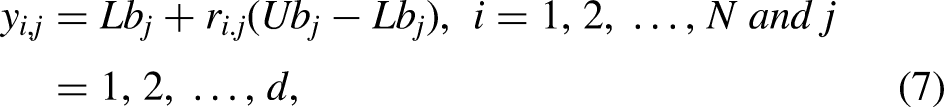
The following makes up the scenario that is presented: The variables N, d, $r_{i.j}$ representing random numbers in the interval [0, 1], $Y_i$ as the $i^{th}$ serval (candidate solution), $L{b}_j$ aand $U{b}_j$ as the lower and upper bounds of the $j^{th}$ decision variable, respectively, and $Y$ as the number of servals are all represented.

Given that each serval represents a potential solution to the problem, the objective function of the problem can be evaluated using the suggested values of each serval for the choice variables. Equation can be utilized to express the values of the objective function of the problem as a vector (8).

$$F={\left[\begin{array}{c}{F}_1\\ \begin{array}{c}⋮\\ F_i\\ ⋮\end{array}\\ F_N\end{array}\right]}_{N\times 1}={\left[\begin{array}{c}F(Y_1)\\ \begin{array}{c}⋮\\ F(Y_i)\\ ⋮\end{array}\\ F(Y_N)\end{array}\right]}_{N\times 1}$$

(8)

In this case, the objective function value calculated from the $i^{th}$ serval is shown as $F_i$ , where F is the vector of objective function values.

The population member who most closely resembles the best value among the computed values for the goal function is the best member of the population. The optimal candidate is determined to be the best value option. It becomes clear that the best member should also be changed as each SOA iteration changes the positions of every population member.

OBL-based opposite weight generation

In OBL, to obtain a more precise approximation of the current solution, the initial serval weight and its opposing serval weight are taken into consideration simultaneously.

$$O{y}_{i,j}=L{b}_{i,j}+U{b}_{i,j}-y_{i,j}$$

(9)

Where $O{y}_{i,j}$ is an Opposite serval weight value, $L{b}_{i,j}$ denotes to the $i^{th},j^{th}$ lower bound, and $U{b}_{i,j}$ denotes to the $i^{th},j^{th}$ upper bound of the given problem solution.

Fitness calculation

Following initialization, every solution's suitability is assessed by the proposed SOA. Here, the assault detection accuracy is defined by the fitness function. The best choice is the one with the highest fitness value.

$$\mathrm{Fitness}=\mathrm{Max}.\mathrm{Accuracy}$$

(10)

Mathematical modeling of SOA

There are two phases involved in upgrading the members of the SOA population in the search area that are modeled after servals’ natural hunting strategy. These phases are meant to resemble the SOA design's local search exploitation phase and global search exploration phase.

Phase 1: prey selection and attacking (exploration)

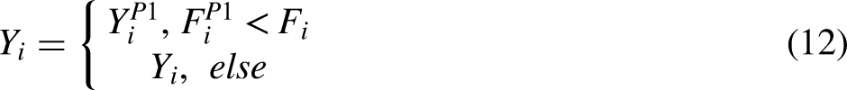
As a skilled hunter, the serval finds its prey by using its keen sense of hearing, after which it launches an attack. The simulation of these two methodologies is used to update the serval positions during the first phase of SOA. This update results in significant serval position modifications and a thorough search space scan. This stage of SOA aims to pinpoint the primary ideal location and boost the exploration's power in the global search. Optimal population member in the SOA design is said to be in the prey position. Equation (11) is initially used to estimate the serval's new position in order to simulate its strike at the target. The old multiple roles are then replaced with the new one in accordance with equation (12) if the new location increases the value of the objective function.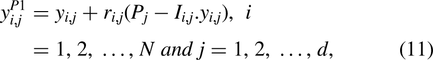

$$y_{i,j}^{P1}=y_{i,j}+r_{i,j}(P_j-I_{i,j}.y_{i,j}),i=1,2,\dots ,Nandj=1,2,\dots ,d,$$

(11)

$$Y_i=\{\begin{array}{c}{Y}_i^{P1},F_i^{P1}<F_i\\ Y_i,else\end{array}$$

(12)

$I_{i,j}$ N is the total number of servals in the population; d is the number of decision variables; the prey location is indicated by $P$ ; its $j^{th}$ dimension is $P_j$ the updated role of the $j^{th}$ serval based on SOA's initial phase is indicated by $Y_i^{P1}$ random numbers in the interval [0, 1]; and the objective function value is $F_i^{P1}$ .

Phase 2: chase process (exploitation)

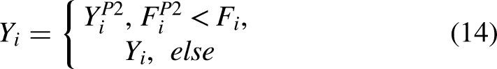
Following an attack, target is pursued by the serval, which jumps on it in an attempt to stop it before killing and eating it. In order to update the population position of SOA, the second stage of SOA makes use of the serval approach. The simulated pursuit process alters the servals’ location inside the search space. Rather, this SOA phase aims to enhance the process of finding solutions and increase the potential of SOA to be exploited in local search (equation (13)). This, when applied to the serval, generates a new random position close to it. This makes it possible to simulate the victim's pursuit by the serval mathematically. Provided that the objective function's value increases due to the new position, equation (14) states that it takes the place of the connected serval's previous location.

$$y_{i,j}^{P2}=y_{i,j}+{\displaystyle \frac{r_{i,j}.(U{b}_j-L{b}_j)}{t},i=1,2,\dots ,Nandj=1,2,\dots ,d,andt=1,2,\dots ,T,}$$

(13)

$$Y_i=\{\begin{array}{c}{Y}_i^{P2},F_i^{P2}<F_i,\\ Y_i,else\end{array}$$

(14)

Here, the new position of the $i^{th}$ serval, as determined by the second phase of SOA, is represented by $Y_i^{P2}$ , $y_{i,j}^{P2}$ is its $j^{th}$ dimension, objective function value is $F_i^{P2}$ , T is the representation of the total number of algorithm iterations, and t is the algorithm's iteration counter.

Process of repetition

After updating every servant in line with the first and second stages of service orientation, the algorithm completes its initial iteration. Based on the revised serval coordinates, the algorithm then moves on to the following iteration using the revised values found for the objective function. Serval position updates are carried out repeatedly up until the last algorithmic iteration, which is based on Equations (11) to (14). Following the completion of SOA implementation, the problem's answer is presented as the best candidate solution found when the algorithm was running.

Termination

Until the optimal weight value or set of values is determined, the process is repeated. The algorithm will end when the perfect serval has been found. Figure 4 shows a flowchart depicting the ESOA installation procedure. The section below provides an explanation of the experimental investigation for the suggested model.

Figure 4.

Flowchart of ESOA.

Experimental framework

The description of the dataset, performance metrics, and system requirements are covered in this section.

Dataset description

The benchmark database is used to evaluate the performance of the recommended approach. Identifying the tumor's location, grade, and kind is just one of the experimental tasks included in this Magnetic Resonance Imaging (MRI) brain tumor diagnosis effort. Br35H, SARTAJ dataset, and fig share are the three datasets combined to obtain this dataset. Size of the images in this dataset is different.

This dataset consists of 7023 human brain MRI scans categorized into four groups: non-tumor, pituitary, glioma, and meningioma.

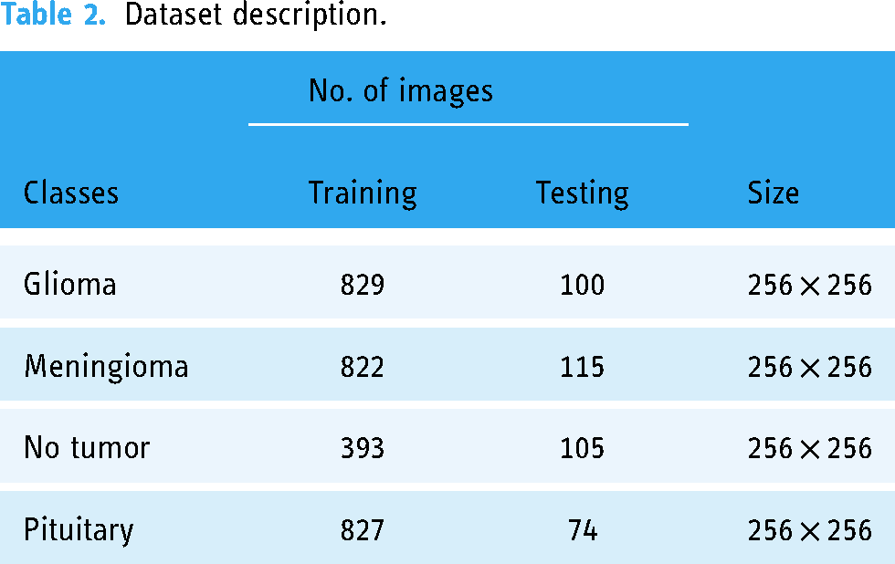
Table 2 provides further details on the datasets. This dataset is divided into four classes: non-tumor, meningioma, glioma, and pituitary. Giloma class contains 829 training and 100 testing images, the meningioma class contains 822 training and 115 testing images, the not tumor class contains 393 training and 105 testing images, and pituitary class contains 827 training and 74 testing images. Moreover, the classes use an image size of 256 × 256 to detect brain tumors.

Table 2.

Dataset description.

Classes	No. of images		Size
	Training	Testing
Glioma	829	100	256 × 256
Meningioma	822	115	256 × 256
No tumor	393	105	256 × 256
Pituitary	827	74	256 × 256

Evaluation metrics

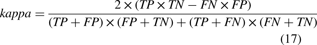
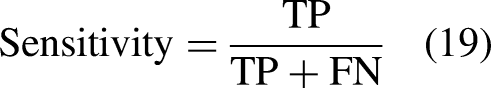
The assessment techniques used in this research were Accuracy (A), Precision (P), F measure, Sensitivity (S), and Specificity (Sp). The following equations represent those methods:

The model's accuracy quantifies how well it recognizes both negative and positive cases.

$$\mathrm{Accuracy}={\displaystyle \frac{\mathrm{TP}+\mathrm{TN}}{\mathrm{TP}+\mathrm{TN}+\mathrm{FP}+\mathrm{FN}}}$$

(15)

The weighted average, or harmonic mean, of recall and precision is known as the F-measure. It provides a comprehensive assessment of a model's effectiveness in terms of precise class predictions.

$$\mathrm{Fmeasure}={\displaystyle \frac{2\times \mathrm{precision}\times \mathrm{Recall}}{\mathrm{precision}+\mathrm{Recall}}}$$

(16)

A statistical metric called Cohen's Kappa, or Kappa, assesses inter-rater agreement in categorical data while accounting for random variance.

$$kappa={\displaystyle \frac{2\times (TP\times TN-FN\times FP)}{(TP+FP)\times (FP+TN)+(TP+FN)\times (FN+TN)}}$$

(17)

Precision is the proportion of true positive predictions a model makes among all positive predictions.

$$\mathrm{Precision}={\displaystyle \frac{\mathrm{TP}}{\mathrm{TP}+\mathrm{FP}}}$$

(18)

The model's sensitivity reveals how accurately it detects positive cases.

$$\mathrm{Sensitivity}={\displaystyle \frac{\mathrm{TP}}{\mathrm{TP}+\mathrm{FN}}}$$

(19)

A metric called specificity indicates how well the model recognizes negative cases.

$$\mathrm{Specificity}={\displaystyle \frac{\mathrm{TN}}{\mathrm{TN}+\mathrm{FP}}}$$

(20)

System requirements

Our experiment was carried out using MATLAB, it was set up on a laptop with an Intel i3 or higher processor and Windows 7 or later, 4 GB or more RAM, and a minimum 500GB hard drive.

Results and discussion

In this part, experimental results of the suggested method are examined. The recommended model is put into practice using the MATLAB workbench. The brain tumor is detected and classified by applying the proposed method to the MRI image. Several performance metrics are computed to assess the proposed brain tumor detection, including F measures, sensitivity, specificity, accuracy, and precision. The training percentage and values of the suggested model are compared with those of several algorithms that are now being used in the investigation. Among these algorithms are Deep Belief Networks (DBN), Oppositional Based Humming Bird Optimization (RNN-LSTM-OHBO), Recurrent Neural Network-Long Short Term Memory-Honey Badger Optimization (RNN-LSTM-HBA), and Recurrent Neural Network-Long Short Term Memory (RNN-LSTM). Below is a depiction of the recommended method's overall output.

A confusion matrix is one deep learning technique for assessing a classification algorithm's efficacy. Use it to assess a model's capacity to distinguish between four classifications for brain tumor identification: “Glioma,” “Meningioma,” “Not tumor,” and “Pituitary.” The ensuing slides show the confusion matrix for the suggested model (Figures 5 to 7).

Figure 5.

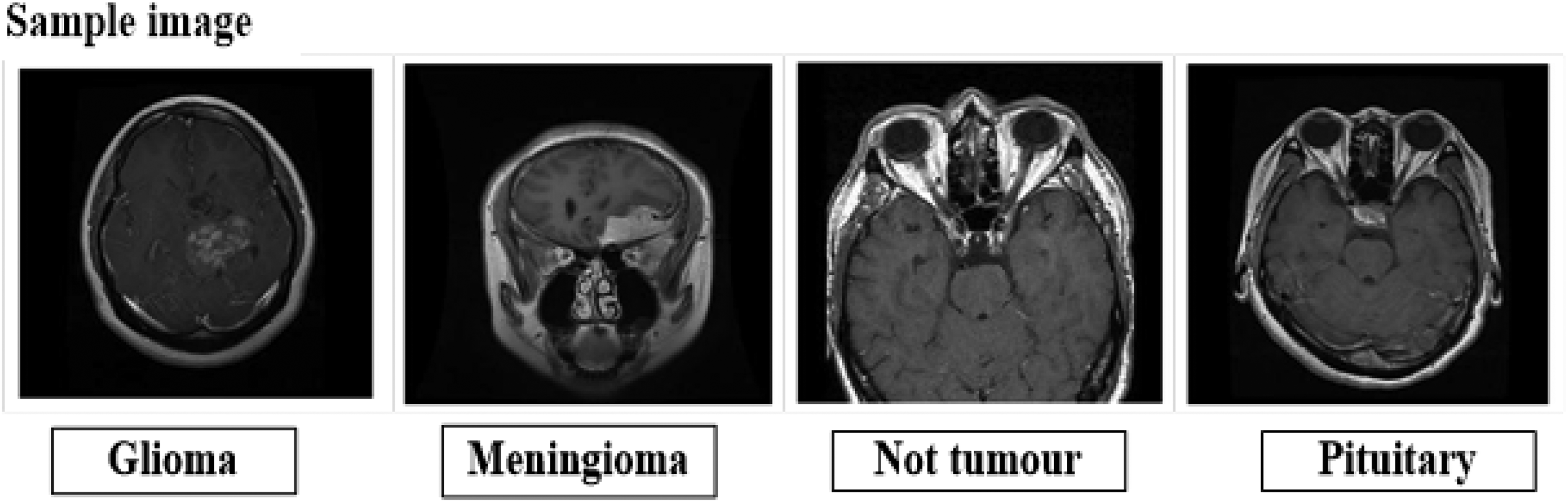
Sample image from the dataset.

Figure 6.

Output of the proposed method.

Figure 7.

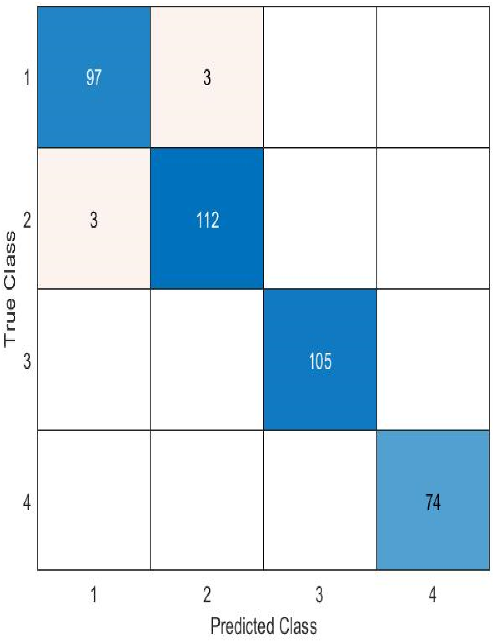
The best-performing ODNN model's confusion matrix.

Figure 8 shows AUC-ROC curves split down by false-positive rates to reflect the true positive rate for each class. The FPR and TPR values are displayed on the respective x- and y-axes for each threshold. The model performs really well, as indicated by the AUC-ROC curve. The optimal classifier is one, AUC and ROC curves’ range is 1.

Figure 8.

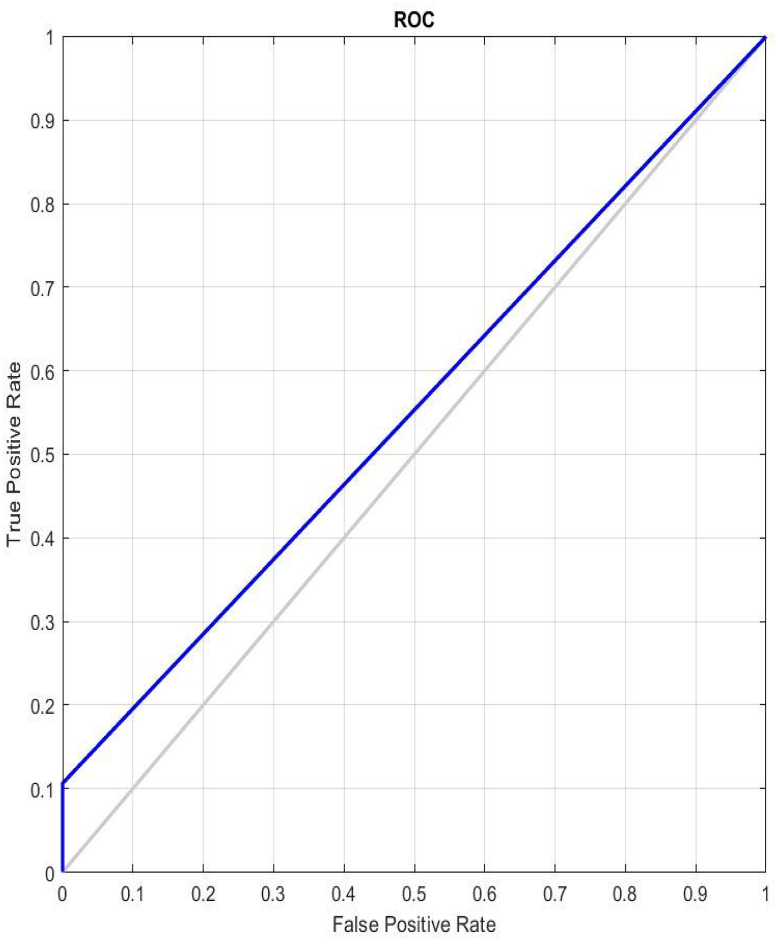
AUC-ROC curve for ODNN.

Comparative analysis

Comparing the suggested method's training percentage and values with those of the different algorithms including RNN-LSTM-OHBO, RNN-LSTM-HBO, and RNN-LSTM and DBNare discussed within this part. The graphs below illustrate the comparison findings of the suggested model. More information on the suggested technique is provided below, along with a comparison of the various qualities of performance metrics.

Figure 9 examines and displays a graphic representation of the projected approach's accuracy measure. It is examined with different training percentages; during 40% of the training percentage, the proposed technique achieves an accuracy of 0.957, whereas the present method achieves 0.947 for RNN-LSTM-OHBP, 0.894 for RNN-LSTM-HBA, 0.895 for RNN-LSTM, and 0.879 for DBN. During 80% of the training percentage, the proposed technique achieves an accuracy of 0.972, whereas the present method achieves 0.962 for RNN-LSTM-OHBP, 0.94 for RNN-LSTM-HBA, 0.929 for RNN-LSTM, and 0.904 for DBN. This evaluation shows that, in comparison to the current methodologies, the suggested approach obtains the best accuracy level.

Figure 9.

Comparision of training accuracy.

An illustration of the predicted approach's F-measure is shown in Figure 10. It is examined with different training percentages; during 50% of the training percentage, the proposed technique achieves a F-measure of 0.923, whereas the present method achieves 0.913 for RNN-LSTM-OHBP, 0.893 for RNN-LSTM-HBA, 0.871 for RNN-LSTM, and 0.841 for DBN. During 80% of the training percentage, the proposed technique obtains a F-measure of 0.954, whereas the existing method achieves 0.944 for RNN-LSTM-OHBP, 0.928 for RNN-LSTM-HBA, 0.900 for RNN-LSTM, and 0.890 for DBN. This analysis shows that, in comparison to the current techniques, the suggested strategy achieves the greatest F-measure level.

Figure 10.

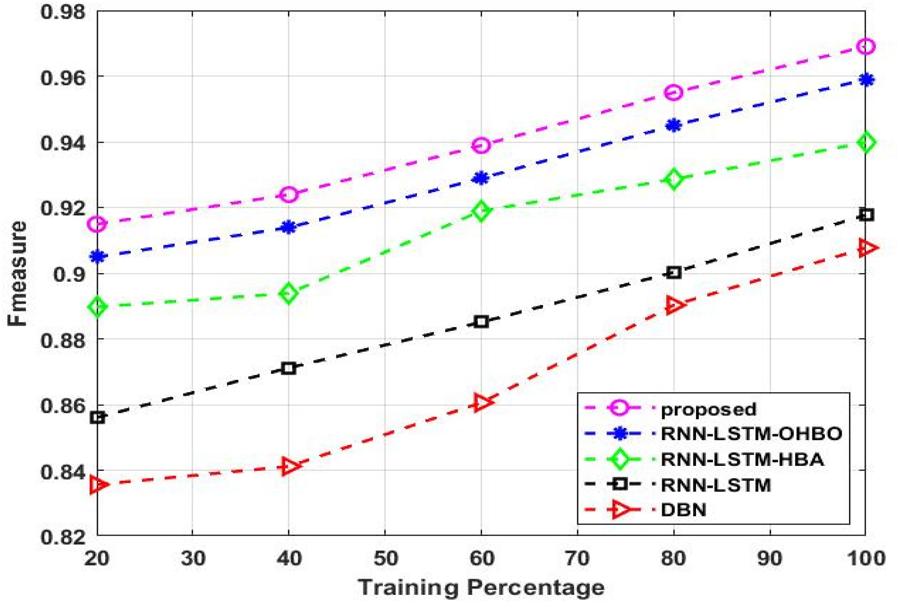
Comparison of F-measure for five models.

Figure 11 shows the kappa of the predicted approach. It is examined with different training percentages; during 40% of the training percentage, the proposed technique achieves a kappa of 0.89, whereas the present method achieves 0.88 for RNN-LSTM-OHBP, 0.87 for RNN-LSTM-HBA, 0.82 for RNN-LSTM, and 0.81 for DBN. During 80% of the training percentage, the proposed technique achieves a kappa of 0.92, whereas the present method achieves 0.91 for RNN-LSTM-OHBP, 0.9 for RNN-LSTM-HBA, 0.89 for RNN-LSTM, and 0.85 for DBN. When compared to the current methodologies, the suggested approach achieves the highest kappa level, according to this evaluation.

Figure 11.

Comparison of Kappa for five models.

Figure 12 examines and displays the precision measure of the predicted approach. It is examined with different training percentages; during 40% of the training percentage, the projected technique attains a precision of 0.901, whereas the present method achieves 0.871 for RNN-LSTM-OHBP, 0.850 for RNN-LSTM-HBA, 0.825 for RNN-LSTM, and 0.793 for DBN. During 80% of the training percentage, the projected technique obtained a precision of 0.936, whereas the present method achieves 0.926 for RNN-LSTM-OHBP, 0.89 for RNN-LSTM-HBA, 0.865 for RNN-LSTM, and 0.818 for DBN. This evaluation indicates that, in comparison to the traditional approaches, the suggested methodology provides the best level of precision.

Figure 12.

Comparison of precision for five models.

The proposed approach's sensitivity is shown graphically in Figure 13. It is examined with different training percentages; during 40% of the training percentage, the proposed technique achieves a Sensitivity of 0.924, whereas the present method achieves 0.914 for RNN-LSTM-OHBP, 0.86 for RNN-LSTM-HBA, 0.858 for RNN-LSTM, and 0.82 for DBN. During 80% of the training percentage, the proposed technique obtains a Sensitivity of 0.94, whereas the present method achieves 0.93 for RNN-LSTM-OHBP, 0.9 for RNN-LSTM-HBA, 0.895 for RNN-LSTM, and 0.88 for DBN. Comparing the proposed approach against the current methods, this evaluation shows that it achieves the highest Sensitivity level.

Figure 13.

Comparison of sensitivity for five models.

A graphic illustration of the projected approach's Specificity measure is examined and shown in Figure 14. It is examined with different training percentages; during 40% of the training percentage, the projected technique attains a specificity of 0.948, whereas the present method achieves 0.938 for RNN-LSTM-OHBP, 0.911 for RNN-LSTM-HBA, 0.891 for RNN-LSTM, and 0.871 for DBN. During 80% of the training percentage, the projected technique obtained a specificity of 0.963, whereas the present method achieves 0.953 for RNN-LSTM-OHBP, 0.944 for RNN-LSTM-HBA, 0.931 for RNN-LSTM, and 0.911 for DBN. This review demonstrates that the suggested strategy achieves the highest level of specificity when compared to the existing methodologies.

Figure 14.

Comparison of specificity for five models.

A comparative analysis of the method's performance measures is shown in Table 3. For each performance metric, we compared the suggested approach to the existing approach. The outcomes clearly show that the proposed performance metrics have the highest values.

Table 3.

Comparison analysis.

Method	Accuracy (%)	F-measure	kappa	Precision	Sensitivity	Specificity
PROPOSED	0.98	0.96	0.94	0.94	0.95	0.97
RNN-LSTM-OHBO	0.97	0.95	0.93	0.93	0.94	0.96
RNN-LSTM-HBA	0.95	0.93	0.92	0.90	0.92	0.95
RNN-LSTM	0.93	0.91	0.90	0.88	0.90	0.94
DBN	0.92	0.90	0.89	0.86	0.89	0.93

The experiment's findings demonstrate the accuracy of the suggested method is higher than that of existing methods at detecting brain tumors. A comparison of the suggested method with multiple research publications is included in the list of results below.

The processing time of the proposed model is presented in Figure 15. The accuracy of the suggested Deep Neural Network is compared with earlier attempts in Table 4. The results demonstrate that the suggested approach achieves 98.8% accuracy when compared to the other distinct research methodology. Due to its utilization of the DNN, the suggested methodology produced better outcomes.

Figure 15.

(a): Processing time (b): DSC and JSC.

Table 4.

Proposed performance comparison of different research articles.

Source	Classification	Accuracy (%)
Shubhangi Solanki et al. 21	CNN	95.40
Mohammad ZaferKhaliki & MuhammetSinanBaşarslan 23	Three layer CNN	98.00
Takowa Rahman et al. 26	Parallel deep CNN	97.33
GökalpÇınarer et al. 35	DNN	95.00
ShenbagarajanAnantharajan et al. 36	Ensemble deep neural Support vector machine	97.93
Seetha et al. 37	CNN	97.50
Anil Kumar Budati& Rajesh BabuKatta 38	SVM	98.13
	KNN	92.13
Proposed	Dnn	98.80

Conclusion

An ODNN was utilized in this work to identify and classify brain tumors based on MRI images. Open source system database was used to assess the recommended method's efficacy. The five phases that make up the proposed approach are augmentation, preprocessing, segmentation, feature extraction of region proposals, and classification. Initially, input image is rotated during the augmentation phase. The following step is pre-processing, when region filling, thresholding, and morphological operations are used. Initially, a thresholding operation, the mean calculation will be performed. In order to eliminate holes from the thresholding output image, morphological activity is followed by a region-filling operation that aims to remove small objects and noise from the background. Next, the pre-processed images will be divided into segments corresponding to the brain tumor using Berkeley's Wavelet Transformation (BWT). Subsequently, Two Channel Convolutional Neural Network (TCNN) will be used for feature extraction of region proposals. After the region is retrieved, it moves on to the classification phase. The Optimal Deep Neural Network will be utilized during the classification stage. Following the extraction of features, DNN structure will be trained and tested. The classifier will utilize the Enhanced Serval Optimization Algorithm (ESOA) to find the optimal gain parameters. Here, the MATLAB programming language is used to implement the recommended model. The effectiveness of the proposed method is assessed based on a set of performance standards, including F measures, accuracy, sensitivity, specificity, and precision. The suggested method has 98.8% detection accuracy for brain tumors. Our goal is to improve the research for future initiatives by utilizing more advanced datasets and deep learning techniques to detect and classify brain tumors.