Sage Journals: Discover world-class research

Abstract

This article describes the emergence of a novel form of capital—which I call “cosine capital”—that finds objectified form in the “embedding” structures of large language models. In the past decade, massive neural network architectures transformed computational approaches to language in the form of large language models. This approach to modeling language is now being adapted to nearly any sequential data structure imaginable in both academia and industry. While these technologies have been hailed as revolutionary, I situate them within a continuous technological and philosophical lineage that runs directly back to the origins of cybernetics and information science, in particular Claude Shannon’s noisy channel model of communication. I imagine this noisy channel as a sort of “diagram of power,” arguing that a similar process of “enclosure” that commodified the bit as the foundational unit of information is now taking place with embeddings, objectifying them as fungible commodities across an increasing range of societal domains. I compare this cosine capital to Fourcade and Healy’s recent notion of “eigencapital,” suggesting that the particular technical features of embeddings—specifically, their inherently relational nature—challenge the eigencapital model and instead represent a fundamentally novel form of abstraction with strong implications for the future of capitalism and technology.

Keywords

Large language models artificial intelligence cybernetics algorithms information theory

Introduction

Large-language models (LLMs) have become a ubiquitous technology since the release of ChatGPT in November 2022. Much like the computer itself, LLMs are expected to code and write for us, parse, organize, and visualize data, provide directions and astrological readings (Hu, 2023), tag and describe photos, and so on.

The structures driving these impressive results have become a source of great fascination among computer scientists and others working with LLMs. Of particular interest is the “embedding,” a vector of numbers that encodes and decodes the knowledge of LLMs. Embeddings may seem like an abstruse and technical concern, but as the technology expands to encompass more and more types of entities—from representations of text and images to behavioral profiles of swipes on dating apps, listening preferences on streaming services, and clicks in browser sessions—they are deeply relevant to any social theory of digital technology. Already in 2017, researchers at Meta declared: “Embed all the things!” (Wu et al., 2017).

Indeed, the fervor around LLMs has led pundits to liken their rise to the early internet era. As the internet was popularized in the 1990s, metaphors and analogies to make sense of the new technology circulated widely. Daniel Bell (1976) dubbed the era after Fordism the “information age,” and the concept gained further footing as the internet opened up an “information superhighway” (e.g. Castells, 1997). As information is counted in bits, this latter concept came to analogize the hopes (e.g. Negroponte, 1995) and fears (e.g. Hayles, 1998) surrounding digital technologies.

Often forgetting that “information” and “bit” have precise mathematical definitions, enthusiasts and critics alike have cultivated wildly hyperbolic theories of the virtual realm. Nevertheless, both parties got something right: digital computing and networking are fundamentally premised on the representation of events as zeroes and ones, and on the measurement of these bits in terms of their average information. Bits and information form the core of all the technologies of the information age, from microprocessors to internet protocols (Gleick, 2011).

Although a technical notion of information was already introduced by Charles Sanders Pierce in the 19th century (Kockelman, 2017), its mathematical and now canonical definition derives from work at Bell Labs in the interwar era, perfected by Claude Shannon in a series of publications in the mid and late 1940s. Along with his contemporaries from the cybernetics movement (Kline, 2015), Shannon was part of early efforts in machine learning and artificial intelligence (AI), devising mechanical mice that could learn to find their way out of a maze (Shannon, 1953), chess-playing robots (Shannon, 1950), and more. Cyberneticists believed that machines could learn complex functions from observation alone, without specific rules or guidelines. Following the “AI winter” from the late 1960s to the early 1980s, this empiricist approach was revived as neural networks and machine learning gained momentum again in the late 1980s (Church and Mercer, 1993; Léon, 2021).

Among practitioners of natural language processing (NLP)—a form of automated linguistics—Shannon’s work inspired many new applications. Beyond the influence of his concepts of bit and information entropy, the guiding metaphor of the time became the “noisy channel model,” the image Shannon conjured to explain how communication could be understood in terms of coding and decoding (Shannon, 1948a). Shannon’s noisy channel provides an early schema for language modeling (Manning and Schütze, 1999) that is still echoed in the “encoder-decoder” transformer architecture (Vaswani et al., 2017) that powers GPT and similar models.

This article revisits Shannon’s information theory to cast light on current-day neural language modeling. I argue that the noisy channel constitutes a “diagram of power” (Foucault, 1995) that organizes the world in terms of bits, information, and now embeddings. By diagram, I mean the forces that determine what can be seen and said in a given social context. In the early internet era, the diagram of the bit meant that various knowledge resources had to be digitized, compressed, stored in databases, and the databases opened to the relevant audience or public. To be seen or transmitted, one had to be digital. Today, embeddings have acquired a similar force in various technical interfaces, naturalized through their central role in wide-ranging sociotechnical settings.

The paper starts with a broad overview on language modeling that connects this particular technical practice to a set of concepts from the social sciences and philosophy of technology. Then, in the first of two main sections of the article, I build on the historiographic idea of two waves of empiricism in NLP—first during the early efforts associated with cybernetics and then the ongoing work after the return of “connectionist” AI in the late 1980s (Church and Mercer, 1993)—to examine Shannon’s information theory and the operation of the bit as a type of material and meaningful translation (Callon, 1984; Kockelman, 2017; Latour, 1990), guided by the idea of “efficient coding.” This, in turn, was formalized through the notion of information entropy. Next, moving on to the second wave of empiricism, I use Word2Vec (Mikolov et al., 2013), an early neural language model, to illustrate how the embedding replicates the bit in the noisy channel, translating streams of tokenized words into high-dimensional word vectors (Brunila and LaViolette, 2022).

Overall, I argue that we can tease out an ideal form of power—new ways of seeing, saying, and knowing—from the language model. At the same time, the embedding represents a more radical form of abstraction, where the code itself becomes meaningful. While the bit set a norm for efficiency, the embedding creates a space of disclosure that determines what is central and peripheral, similar and dissimilar, significant and insignificant. Instead of a “precise set of digital records” (Fourcade and Healy, 2017: 4), embeddings only require a stream of data tokens, which lend themselves to even greater levels of abstraction (Toscano, 2008). Anything that can be represented as a sequence can be embedded, and the power to do so gives rise to a new type of resource: cosine capital. Here, embeddings are to LLMs what bits were to the digital computer: the basic units that encode what is possible, true, and valuable in a system. However, embeddings become capital only when they are mobilized, producing “meaning in motion” similar to how Marxist theory conceptualizes capital as “value in motion” (money is exchanged for commodities, which are exchanged for more money) (Marx, 1993).

I close the article with a discussion that contrasts cosine capital to the more general notion of what Fourcade and Healey call “eigencapital,” that is, “any form of capital arising from one’s digital records” (Fourcade and Healy, 2017: 2). Whereas eigencapital relies on naming and ordering (Fourcade and Healy, 2024: 105–108), cosine capital emerges from the machine semiotics (Schaffer, 1994) of data where dimensions have neither name nor meaningful order. Consequently, identifying the accumulation of cosine capital through embeddings in the expanding “stack” (Bratton, 2016) of socio-technological infrastructures requires a novel and more precise set of concepts, of which I hope this article can provide an initial outline.

Background: Seeing like a language model

Language models proceed first and foremost by answering the question: “Given some set of context words, what is the most likely next word?” It makes these predictions on the basis of linguistic patterns in large corpora, using statistical methods and machine learning. Once “learned,” these patterns can be used to predict or generate new words conditional on some context words, like the kind of prompt one gives ChatGPT. Prompted with “the cat sat on the,” a simple language model trained on common English phrases will probably predict “mat” as the next word, as it knows this example from the training data.

Enclosure and disclosure

To theorize the operation of these next-word prediction systems, I rely on the notions of enclosure and disclosure (Kockelman, 2017). When a model is trained on a corpus of training data, that corpus is enclosed by the model. When that model generates new language from an input prompt, it discloses from the model, revealing what can be said, and how. For instance, Google’s Gemini model refused for a long time to answer the question “Where is Gaza” (e.g. Navlakha, 2023). Due to “safety concerns,” many LLMs also refuse to give particular advice about issues like self-harm or explosives, unless prompted in very specific ways. By engineering particular prompts, LLMs can be “jailbroken” to make certain disclosures, but even then only on the condition that the necessary words have somehow been enclosed (Kockelman, 2013: 126). While it may seem that enclosure applies primarily to the selection of training data, the example of the question “Where is Gaza” demonstrates how sequences can also be retroactively excluded from the domain of a model.

On a general level, enclosure defines what exists (ontology) and determines the domain of disclosure, that is, what can be said, seen, and known (epistemology). In this sense, enclosure requires an exercise in distinguishing forms (Bryant, 2011). It demands that we ask: what are the fundamental units, that is, the individual “tokens,” that the model can know? How do we translate (Callon, 1984; Latour, 1990) spoken or written text into model inputs? Which words and contexts exist in the world of the model, and which do not?

The meaning of meaning

During model training, the model continuously makes predictions that improve its weights—the parameters that convert a given input to a given output—relative to some information metric, such as cross-entropy, a technical concept I revisit below. An embedding is simply a collection of these weights that encodes the variations in observed distributions between words. Words that appear in similar linguistic contexts (e.g. “dog” and “cat”) will have similar embeddings. This idea that the meaning of a word is somehow embedded in its observed distribution relative to other words is old.¹ In neural language modeling, this idea is reflected in the conflation between distributional similarity and meaning: the more similar the embeddings of two words, the more similar the words are in meaning (e.g. Mikolov et al., 2013; Pennington et al., 2014). Here, meaning is detached from external referents and normative definitions, empirically derived (Harnad, 1990) from co-occurrence statistics alone. To the question “What is the meaning of this sequence of words?” one can simply answer: “Whatever is predicted next by the model!” Which words are similar in meaning? Words with similar embeddings! This is the empiricist answer to the classical question: “What is the meaning of meaning?” (Ogden and Richards, 1923). While rationalists like Chomsky started with clear hypotheses about the human mind and language, within the contemporary paradigm of AI the only hypothesis is distributionalism, that is, the “empiricism” of data (Church and Mercer, 1993; Henderson, 2020).

Under distributionalism, the process that guides LLM training is self-supervised. While supervised learning is measured against predetermined “ground-truth” labels (e.g. ham or spam for emails, parts-of-speech for words), in self-supervision “labels are created by the algorithm, rather than being provided externally by a human” (Murphy, 2021: 626). The “labels” for a word are none other than the observed context words that precede it (next token prediction) or surround it (masked prediction).

The world of the LLM

The world of the language model is determined by the tokens and types (the unique tokens in the vocabulary) it knows. Even words that are not predicted in a given context matter by defining the space of possible predictions. Merely by being possible, they lend meaning to the word that was actually predicted (“A” defined as not “B,” “C,” “D,” etc.) (Luhmann, 1990), the space of metric and structural information from which selective information is drawn (MacKay, 1969). In Saussurean terms, predictions progress along a “syntagm” that gains its meaning from the “paradigm” of plausible choices (Jakobson and Halle, 2002). Here, the paradigm is the world of the model, its realm of ‘‘possibilities” (what could happen/be predicted), while the syntagm is like the progress of history (what actually happened/was predicted). The predicted word expresses a statistical norm conditional on the context words. Probable words are, well, more probable, and in the aggregate they will predominate, again, conditional on the given context. This trend has been noted in recent empirical studies on LLMs, which have observed that LLM-generated language narrows over time. This kind of “model collapse” happens progressively, as GPT-n+1 is trained on inputs from GPT-n. Language regresses closer and closer to the mean, erasing its long tails (Shumailov et al., 2023).

Cosine capital: Embed all the things!

This approach to the modeling the meaning of entities within an enclosed system is no longer limited to linguistic semantics. Self-supervision techniques are being applied to wide array of “events.” Anything sequential can be embedded, made to self-supervise: clicks during a browser session (Grbovic and Cheng, 2018), genetic code (Ji et al., 2021), people on a dating app (Liu, 2017), songs streamed over the course of a party (Hansen et al., 2020). While Figure 1 demonstrates the production of training data for a language model, Figure 2 provides a contrasting example from a very different domain. Here, Tinder “swipers” are represented through embeddings formed by the swipes that they receive. Similarly, Figure 3 shows how Airbnb listings can be represented by embedding the clicks they receive. The listings in the figure are similar because they appeared in similar sequences of clicks on the website, which turns out to be a good proxy for their actual attributes (location, size, type, etc.).

Figure 1.

The sliding window of Word2Vec Skipgram algorithm. One-by-one, words serve as the target (green) from which the context (orange) is predicted.

Figure 2.

In a presentation at the machine learning conference MLConf, researchers at Tinder (Liu, 2017) explained how users can be represented simply using their swipes. Here, users that get swipes from one user provide the context for each other, much like words appearing in a specific sentence.

Figure 3.

A research paper by the data science team at Airbnb (Grbovic and Cheng, 2018) demonstrates how Airbnb listings can be represented through comparing clicks in a browser-session. Rather than represented through their qualities (size, location, etc.) these listings are similar because they appear in similar browser sessions. They are not represented by their attributes, but the embeddings results from a particular behavioral pattern.

Cosine similarity: The semantics of embeddings

Here I introduce the notion of cosine capital in order to theorize the power to embed. This concept is derived from a mathematical and social understanding of embeddings through their (1) cosine similarity to one another and their (2) accumulation as capital.

Recall from above that embeddings are representations of words (or other sequentially arrayed units) in a vector space. Computationally, two words are similar in meaning if their embeddings have a high cosine similarity. Embeddings were introduced already in the 1950s in the context of social psychological studies that categorized words along axes such as “happy”/“sad” and “hard”/“soft” (Jurafsky and Martin, 2021) and later in computational linguistics to represent documents via word counts. In the latter case, documents with similar words would have similar embeddings. However, modern-day embeddings are not defined along dimensions that make sense for the human interpreter. Instead, embeddings are defined along the arbitrary dimensions of the matrices that contain the neural network weights.

These modern embeddings are thought to capture latent knowledge expressed by language, from simple analogies such as the oft-cited example “king is to queen as man is to woman” (Pennington et al., 2014) to lexical markers correlated to complex social relations and phenomena ranging from social class (e.g. Kozlowski et al., 2019) and gender (e.g. Garg et al., 2018) to gentrification (e.g. Brunila et al., 2023) and political ideology (e.g. Rheault and Cochrane, 2020).

Cosine similarity compares embedding vectors by measuring the angle between them, at values between $-$ 1 and 1. At $-$ 1, two embeddings are opposite to each other, at 0 they are orthogonal, and at 1 they are identical. In principle, values close to $-$ 1 and 1 should indicate antonymy and synonymy, respectively, while embeddings with a cosine similarity of 0 should be completely unrelated. However, in practice, embeddings are famously poor at detecting negation and antonymy (e.g. Truong et al., 2023).

Embeddings as capital: Meaning in motion

Anyone with embeddings trained on large amounts of data possesses cosine capital. However, in Marx’s (1993) classical formulation, capital is not just value, but value in motion. We saw above how embeddings become a de facto repository of what is considered meaningful in a growing set of technical systems, but how are they “in motion”?

For Marx, capital is characterized by the formula M-C-M $^{'}$ , where money (M) is exchanged for some commodity (C), which is then sold for more money (M $^{'}$ ). Extending this to cosine capital, we can understand it as vectorized meaning in motion. Embeddings (E) fuel the generation of new “content” (C) (words, images, music, dating profiles, recommendations, etc.), which prompt human users to provide responses which then are used to train more embeddings (E $^{'}$ ), resulting in the cycle E-C-E $^{'}$ . Interfaces like ChatGPT and Gemini are perfect examples of this dynamic. Another way of understanding this cycle is in terms of encoding/enclosure (E) and decoding/disclosure (D), or E-D-E $^{'}$ (for a summary of these movements, see Figure 4). Embeddings themselves are not cosine capital, just like money itself is not capital, and (presumably) data alone is not eigencapital. Only in circulation does each of these become realized as capital (Heinrich, 2012).

Figure 4.

For Marx, capital is not something one can hold, but value in motion. The capitalist starts with money, invests it in a commodity with the purpose of selling that commodity for more money or “money prime” (money $^{'}$ ). Similarly, cosine capital is “meaning in motion.” On a pragmatic level, a user of ChatGPT prompts the embeddings of an underlying model. These prompts and interactions with the model produce content, which can be used to train more models, to produce more embeddings or “embeddings prime” (embeddings’). This is also a process of form turning into meaning and into “form prime” (form $^{'}$ ). It is likewise a process of encoding, decoding and “encoding prime” (encoding $^{'}$ ), and, furthermore, a process of enclosure, disclosure, and “enclosure prime” (enclosure $^{'}$ ).

As capital, embeddings are not just a source of power but a formative social force. As demonstrated in his analysis of the factory, Foucault understood the operation of capital as a “diagram” (Deleuze, 1999; Foucault, 1995: 205). Foucault originally brought up these analogous concepts in his analysis of disciplinary power and the architecture of the Panoptic prison in particular. Understanding the Panopticon as a diagram of power did not cast it as “a dream building,” but rather “the mechanism of power reduced to its ideal form” (Foucault, 1995: 205). Similarly, money operates as a diagram of the value form that forces both human and non-human forms of life to express themselves in terms of their exchange value.

Embeddings are likewise making the world in their image through innumerable technical applications. It is in this sense that language modeling becomes a diagram of power: the embedding functions as a universal representation of any sequence, encoding meaning while simultaneously obfuscating (Burrell, 2016) it in the enigma of its own uninterpretable dimensions.

From bits to embeddings: Two waves of data empiricism

In more material terms, a natural point of contrast for the embedding is found in the bit, arguably the most fundamental unit for representing data and measuring information. In this section of the article, I focus on the historical and technical continua and ruptures that characterize the development of the embedding from the foundations of the bit. The bit serves as the pivot for a set of innovations—characterizing data through information entropy, understanding communication as the coding and decoding of a noisy channel, and comparing distributions via cross-entropy—that were developed not only to represent data, but also to evaluate how efficiently it is represented.²

Embeddings are much like bits, but explicitly semantic. This means that embeddings that are similar (as measured by the cosine of the angle between the vectors) should represent things that are themselves similar. They rely on the key innovations that made the bit sensible—as has been noted in recent technical literature on LLMs (Delétang et al., 2023)—but explicitly capturing the semantic aspects of data. In this sense, one could argue that they are “semantic bits,” relying on similar metaphors of communication but elevating them to new and arguably higher levels of abstraction. This is hardly a coincidence, as the embedding seems to extend and “semanticize” the paradigm of data processing that we have all come to know through our personal computers and smartphones. The embedding provides an affordance for the quantification of meaning, moving past the original commitment in information theory to ignore semantics and focus on the “engineering aspects of information” (Shannon, 1948a).

The following two sections of the article start with a brief overview of how NLP returned to the “empiricism” of Shannon and others in the 1990s, followed by a more detailed technical and historical exploration of the bit in early information theory. Then, before moving to the discussion, I demonstrate the historical continuum between the bit and the embedding and clarify the technical aspects that both connect and put the embedding apart from the bit.

The empiricism of the bit

NLP: From bits to embeddings

The influence of cybernetics on NLP can be traced through the evolution of both computer science and linguistics, a historical connection that is widely recognized in the canonical textbooks of AI (e.g. Goodfellow et al., 2016; Russell and Norvig, 2020) and NLP (e.g. Jurafsky and Martin, 2021; Manning and Schütze, 1999). Firstly, modern neural networks and the backpropagation algorithms used to train them are also based on innovations from cybernetics, including notions of feedback and information proposed by Norbert Wiener and Shannon as well as the McCulloch-Pitts neuron and the Perceptron model. Secondly, by way of “distributional semantics,” structural linguistics—which was deeply influenced by information theory (Brunila and LaViolette, 2022)—provided theoretical support for the idea that meaning is a function of redundancy in lexical patterns.

In the NLP literature, the connection between cybernetics and the current wave of neural approaches has been presented as a return to the “empiricist” roots of the discipline in probabilistic methods and information theory (Church and Mercer, 1993; Léon, 2021: 141; Norvig, 2012). In a 1993 ‘‘Special Issue on Computational Linguistics Using Large Corpora” for the Association of Computational Linguistics (ACL), the authors noted that “[s]tochastic methods based on Shannon’s noisy channel model have become the methods of choice within the speech community” (Church and Mercer, 1993: 2). In the first modern textbook on NLP, the authors similarly noted that “it was research into speech recognition that inspired the revival of statistical methods within NLP, and many of the techniques that we present were developed first for speech and then spread over into NLP” (Manning and Schütze, 1999: xxx). Moreover, Shannon had, in fact, been one of the first people to formalize the language modeling problem (Shannon, 1945, 1948a, 1951). It is unsurprising that language modeling was habitually called the “Shannon game” until the 1990s (e.g., Manning and Schütze, 1999; see also Brunila, 2024).

Metaphors of communication in information theory

Linguists have noted how Shannon’s information theory was premised on the idea of communication as a “conduit” that carries ideas that the reader simply needs to decode (Reddy, 1993). Shannon articulated this metaphor most clearly when, in his later work (Shannon, 1948a, 1948b), he suggested that communication works as a “noisy channel” of sequential transformations, encoding a set of messages into some domain—like Morse code—and then decoding them into the original message. This channel is “noisy” because it often introduces some error through disruptions in the transmission (see Figure 5).

Figure 5.

Shannon’s schematic diagram of a general communication system (Shannon and Weaver, 1963: 34).

In an early sketch, (Figure 6), Shannon illustrated clearly how the noisy channel would cast communication as a sequence of functions that transform each other in succession.³ In the diagram, each function takes an input and transforms it into an output. Here, communication starts with the emission of a set of messages, where at each moment $t$ in time there is an output that is determined by some function $f_{1}$ . This output is, in turn, processed by the function $T$ , which produces the signal $F (t)$ “which is actually transmitted.” Then,“ $F (t)$ enters the receiving element $R$ and is there transformed into a third function of time $f_{2} (t)$ .” This last function, Shannon stressed, “should be as closely similar to $f_{1} (t)$ as possible,” that is, reproducing the original input.

Figure 6.

Shannon’s first sketch of a diagram of “all systems of communication” (Shannon, 1993: 455) showed communication as a sequence of mathematical functions.

Encoding and decoding messages

Shannon’s idea of communication must be understood in the context of his work as a cryptographer during World War II, when he was tasked with producing algorithms for encoding and then decoding messages securely on the receiving end (Soni and Goodman, 2017: 149–151). The task was not merely to conceal language, but to do so in a way that made it possible to re-discover it later on. This kind of “practical secrecy” (Shannon, 1945) finds the functions that encode a message so that it can still be deciphered, given the correct key. If, for instance, the message “oxford” is encoded with a simple substitution cipher as “FJKFPO,” then several English words are possible messages, including “thatis,” “ofyour,” and “season” (Damm and Brosenne, Winter 2013/2014). Both the message and the cipher have a similar probability distribution for their respective symbols. They are structurally isomorphic, with similar statistical structure or redundancy, “a series of conditions on the letters of the message, which insure that it be statistically reasonable” (Shannon, 1945: 21). These “consistency conditions” for the message produce, in turn, “consistency conditions in the cryptogram” (i.e. the cipher from above). The code needs to be consistent with the message: there is a certain amount of freedom of choice that can be exercised in making the code.

Quantifying words as bits

With communication understood as a system of coding and decoding, a natural question follows: How could one characterize, design, and break the codes of such a system? Shannon acknowledged that the “significant aspect is that the actual message is one selected from a set of possible messages” (Shannon, 1948a: 379), making information a measure of the tension between a selected symbol and all possible symbols. This measure, Shannon insisted, was purely technical:

Frequently the messages have meaning; that is they refer to or are correlated according to some system with certain physical or conceptual entities. These semantic aspects of communication are irrelevant to the engineering problem. (Shannon, 1948a: 379)

Instead of the messy worlds of semantics or psychology, the “problem” that the mathematical theory of information addresses is the overall “uncertainty” of a system and its codes (Shannon, 1945: 7).

To illustrate his theory, Shannon imagined an “artificial language” (Shannon, 1948a: 387), with only the four equally likely letters A, B, C, and D—each with the probability of $0.25$ . Shannon wanted to characterize this entire distribution of probabilities in order to measure how much “choice” the communication system has as it selects a letter. The more choice, the more surprising each letter or system state should be. This notion of choice could be thought of in terms of the number of “yes” or “no” questions we would have to ask until we know which “event” (A, B, C, or D) occurred (Shannon, 1945: 10, 58). These questions were called “bits,” so that a single bit is effectively a question that invites us to answer “yes” or “no,” $0$ or $1$ (Shannon, 1948a: 380).

The more questions we need to ask, the more bits are needed to describe a system. For the artificial language from above, we could first ask “is it A or B?.” If the answer is “yes,” we can ask “is it A?.” If the answer is “yes” we know it is A, if the answer is “no” we know it is B. If the answer to the first question was “no,” then we can simply repeat the procedure for “C” and “D.” In each case, we need only two questions to find out the correct symbol. Since we can, on average, find out each event with two questions, the system itself can be characterized with two bits (see Table 1). With eight characters, we would need three bits. Shannon proposed that this logic could be formalized through the equation for entropy from statistical mechanics (Shannon, 1945: 10) (for mathematical details on entropy, see Appendix A).

Information measures, in short, the presence of structure in the possible states of a system. When there is little or no structure, events (i.e. changes in state) are more “informative.” When events are very structured or even predetermined, each event is redundant and “uninformative.” Information is synonymous with surprise; a draw from a distribution with uniform probabilities will on average be more surprising than a draw from a more skewed distribution.

Table 1.

These kinds of bit tables were common in early information theory (e.g. Fano, 1950; Shannon, 1948a).

Outcomes	Probabilities	Bits	N bits	Weighted bits
A	0.25	00	2	0.5
B	0.25	01	2	0.5
C	0.25	10	2	0.5
D	0.25	11	2	0.5

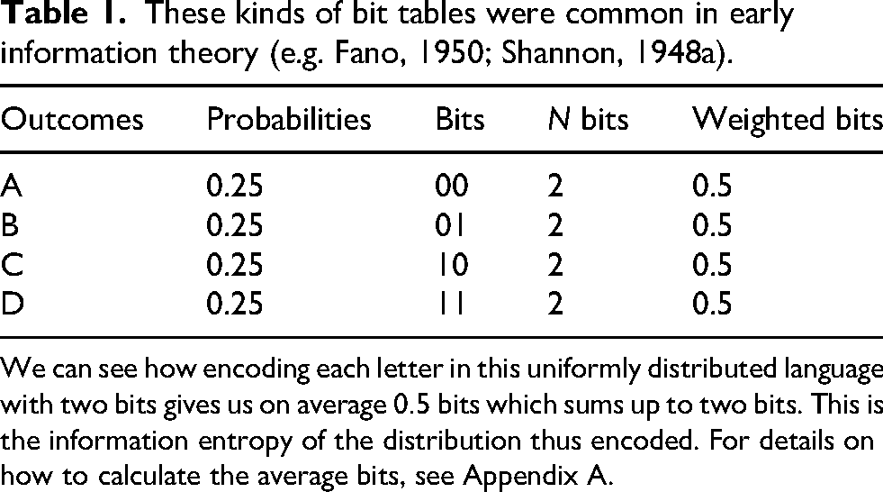
We can see how encoding each letter in this uniformly distributed language with two bits gives us on average $0.5$ bits which sums up to two bits. This is the information entropy of the distribution thus encoded. For details on how to calculate the average bits, see Appendix A.

Entropy as the measure of efficient bit encoding

The bit provides a parsimonious language for describing the set of possible states in a system. What the bit does not provide is a pathway for actually figuring out how to allocate bits in order to describe a system effectively.

Given any physical system of communication, such as telephony or telegraphy, the system itself presented a limit at which it could process incoming signals. This fact already informed the design of Morse code, which allocated signals based on the statistical regularities of the English language. In Morse, “E,” the most common letter in the English language, is simply a dot (.), while a less common letter such as “Q” is dash-dash-dot-dash (- - . -). Shannon realized that the most effective code of them all could be precisely determined using the statistical regularities of language so that the average number of bits (entropy) needed for encoding the messages were minimized.

But how could these statistical regularities be found? Cryptographers had long consulted manually compiled frequency tables of words and letters when constructing cryptograms (Kahn, 1996). Initially, Shannon did too. However, by 1951 Shannon had devised a set of experiments where human subjects (including his wife, Betty) tried to guess letters that had been removed from a sentence (Shannon, 1951). By considering such predictive faculties of humans, Shannon thought he could find upper and lower bounds for the information entropy of the English language. This is the “Shannon game,” as language modeling was long called (Brunila, 2024).

Shannon speculated that this kind of learning could be automated, even designing a device where a mechanical mouse (Shannon, 1953) running through a maze on top of telephone relays “learned” the correct relay design to find its way to a wooden piece of cheese. There existed a correct or “efficient code” for any system, whether a language or a robot mouse. Ergo, the most efficient code and some subpar estimation of it could also be compared. If a language was actually very structured, then assuming a lack of structure would lead to inefficient coding. By comparing the assumed and actual codes, we can know how far we are from the optimal encoding of our messages. In this way, the very idea of information heralds a particular notion of efficiency and structure: the ideal bit representation accounts for the observed, empirical probabilities of language, with the aim to minimize the number of expended bits.

To demonstrate this, Shannon once again considered the language A, B, C, and, D, now with varying probabilities (see Table 2 and Appendix B for details). We need on average $\frac{7}{4}$ bits to encode each letter in this example (see Table 2(b)). Remember, one bit is just a “yes” or “no” question. To “encode with bits” means translating the probabilities of our language into these types of questions (even if they are fractional).

Table 2.

Two ways to encode a hypothetical language with the symbols A, B, C, and D and the corresponding independent probabilities $0.5, 0.25, 0.125, 0.125$ , respectively.

(a) Maximum entropy encoding
Outcomes	Probabilities	Bits	N bits	Weighted bits
A	0.5	00	2	1
B	0.25	01	2	0.5
C	0.125	10	2	0.25
D	0.125	11	2	0.25

(b) Optimal encoding
Outcomes	Probabilities	Bits	N bits	Weighted bits
A	0.5	0	1	0.5
B	0.25	10	2	0.5
C	0.125	110	3	0.375
D	0.125	111	3	0.375

With the maximum entropy encoding (a) each symbol requires on average $2$ bits, with the optimal encoding (b) each symbol requires on average $\frac{7}{4}$ or $1.75$ bits. The relative entropy between the two coding schemes is $\frac{2}{\frac{7}{4}} = \frac{7}{8}$ or $0.875$ bits, which is our compression ratio (Shannon, 1948a: 404–405).

How good is the encoding? Measuring with cross-entropy loss

What if we did not know the probabilities of the symbols in this language and instead approach this language like the mouse in Shannon’s maze, bumping into walls, guessing our way forward? Much like the mouse, we would start by assuming that the structure is random, that is, that each letter has the same probability $0.25$ . Here, language is completely unstructured, a “maximum entropy source” (Shannon, 1948a: 404) (see Table 2(a)).

Assuming that our language—just like the first example—is a maximum entropy process, we need on average two bits to encode each letter. This is more than the optimal $\frac{7}{4}$ bits. Our encoding is, in other words, inefficient. The intuition can be seen in Table 2: encoding all four symbols with an average of two bits is only efficient if the symbols are equally probable, which they are not. Conversely, if all the symbols were equally probable, then encoding each of them with two bits would be more efficient than the alternative (Murphy, 2021: 243). In fact, an optimal coding scheme will allocate fewer bits to more probable symbols and more bits to less probable symbols (Murphy, 2021: 243).

Furthermore, by comparing the actual code to the maximum entropy code, we can determine how much our language can be “compressed,” that is, how much more efficiently it could be encoded (Shannon, 1945: 20; Shannon, 1948a: 398). These results from Shannon were eventually extended by others. In 1951, mathematicians Solomon Kullback and Richard Leibler wrote that the “statistical problem of discrimination” between two distributions and the “‘divergence’ between statistical populations” can be measured by generalizing Shannon’s theory “to the abstract case” (Kullback and Leibler, 1951: 79).⁴ Cross-entropy (Goodfellow et al., 2016), the most common “objective” or “loss” function in NLP, is a special case of the metric they developed, and measures a type of “information divergence” between two distributions of probabilities over the same set of symbols: one empirical, observed distribution, and one estimated distribution. The most efficient code, in other words, is the code that minimizes the divergence and encodes symbols with the average bits dictated by the empirical distribution of probabilities.

The empiricism of the embedding

It is perhaps in this problem of allocating the optimal bit encoding that we can most clearly perceive the continuity between bit and embedding. In 1993, when the “return to empiricism” was declared in the ACL special issue, the comparison of ideal and empirical distributions through cross-entropy was front and center. “Cross-entropy is a useful yardstick for measuring the ability of a language model to predict a source of data,” Kenneth Church and Robert Mercer (1993: 13) noted in their introduction to the issue. The statement was prophetic: today, cross-entropy is what orients the mouse in the proverbial maze of machine learning with lexical data.

Church and Mercer imagined, following Shannon, that a language could be represented by the average bits needed to encode each symbol:

One can also think of the cross-entropy between a language model and a probabilistic source as the number of bits that will be needed on average to encode a symbol from the source when it is assumed, albeit mistakenly, that the language model is a perfect probabilistic characterization of the source. (Church and Mercer, 1993)

Presaging contemporary approaches, Church and Mercer proposed a scenario where two samples of linguistic data were collected: one to fit values of the parameters of the bit encoding (today the “train set”), and another used to test how well these parameters predicted symbols (today the “test set”). To illustrate the point, they compared the number of bits required when using different encoding schemas on a sample from the Wall Street Journal. ASCII required 8 bits and Huffman coding each word took 2.1 bits. Shannon had estimated that human performance was at 1.25 bits (Church and Mercer, 1993: 14). Better word representations by machine were still possible.

Quantifying words as vectors

For a statistical language model to see words, they have to be digitally represented or “enclosed” for the model. During the 1990s, words were generally represented as very large vectors of zeroes and ones. These “one-hot encoded” vectors were the size of the vocabulary in the data, each vector having a $1$ for the word it represented and a $0$ in all other positions. These vectors are like bits, but with thousands of entries, one of them $1$ , and the rest $0$ . Documents could also be represented by augmenting these numbers, so that a document with three occurrences of the word “dog” would be represented by a vector with the number $3$ in the position corresponding to “dog” and $0$ in all other positions. Each word in the document was assigned this type of “count vector.” While unwieldy, these structures translate well between human and computer semantics.

However, these word vectors suffered from what in the discipline is known as the “curse of dimensionality”: When there are more dimensions to a given vector than there are actual training samples in the data, models become volatile and unreliable (Goodfellow et al., 2016: 156–157). Consequently, “as the volume of space grows exponentially fast with dimension,” you might have to look quite far away in the embedding space to find the nearest word (Murphy, 2021: 542–543).

One solution to this problem was offered by Yoshua Bengio and colleagues (2000) in a landmark paper that suggested that neural networks could be used to learn compressed and “distributed representations” of words. By learning word representations instead of just assigning them, words could be compressed into a smaller space, where each word was represented by a much smaller vector of floating point values⁵ instead of a very large vector of integers. Suddenly, through the distributed representation, prediction became the engine for finding the perfect representation. Instead of assigned bits, words were given learned embeddings.

Encoding and decoding with word vectors

While Bengio et al. demonstrated a significant improvement in performance on the language modeling task of next token prediction, they paid little attention to one detail: what kind of knowledge was expressed in these learned vectors? Nevertheless, it is this detail that marks the transition towards the “semanticization” of information.

The semantic characteristics of these learned vectors or “word embeddings” were taken up by several research teams in the early 2010s. Two seminal papers in particular, one from Google (Mikolov et al., 2013) and the other from Stanford (Pennington et al., 2014), took the NLP world by storm. Of the two papers, the one by Mikolov et al. at Google was a particularly clear extension of the noisy channel approach to language modeling. Figure 7 shows Word2Vec interpreted as an instance of a noisy channel.⁶

Figure 7.

Adapting Shannon’s noisy channel schema to describe Word2Vec. The text on top of the boxes replicates Shannon’s own terminology. Inside the boxes is terminology more aligned with the wording in this article, with the parenthesis providing the dimensions of the vectors and matrices at each step. $V$ is the size of the vocabulary and $N$ is the size of the embeddings. The small text snippets on the bottom provide more technical details. The target word is the input message, which is encoded using the target embedding matrix. This gives us the signal of the hidden layer. Multiplying the hidden layer with the decoder matrix of context embeddings, we get a vector of predictions. This vector is passed through the softmax function to get a final normalized vector of probabilities. This prediction of most likely context words is the final output message. For a detailed example, see Figure 8 (the encoder) and Figure 9 (the decoder).

The basic idea of Word2vec is simple. Given a text, a sliding window is moved over each word, along with some $n$ neighbors to the right and left. As the window moves, the context words to the left and right are removed and the model tries to guess what the removed words are, given the center “target” word (see Figure 1). Looking again at Figure 7, we can see that the target word is the input “message,” with the context words appearing as the output “message.” For this task, Word2Vec utilizes a simple feed-forward neural network architecture.⁷

I demonstrate the operation of this architecture on one training sample in Figures 8 and 9. First, all target words are encoded using a matrix, where each word is represented by a floating point vector of some arbitrary length, usually between 50 and 300. If the words are given 50 numbers each and there are 10,000 words, then the matrix is 10,000 rows (one for each word) by 50 columns (one for each dimension of the vector). This is the encoder. In our example (Figure 8), we have only eleven unique tokens (i.e. types) in our example ( $V$ in Figure 8), each with an embedding of just three dimensions ( $N$ in Figure 8).

Figure 8.

The encoder part of the Skipgram algorithm in Word2Vec. In this example, we are given the word “communication” to predict words in a context window of size $1$ , so we should predict the words “of” and “are.” We start by taking the one-hot representation of “communication” and multiplying it with the matrix of randomly initialized embeddings. This gives us the embedding for “communication,” which is our signal. For the decoder part, see Figure 9.

Figure 9.

The decoder part of the Skipgram algorithm in Word2Vec. We take the signal word “communication” and multiply it with the matrix of context embeddings, which before we have trained our model is just a random initialization. This gives us a vector of predictions, which we normalize into probabilities using the softmax function. Since our context window was two, we pick the two most likely candidates, our predicted message, which at this point are “semantic” (0.35 probability) and “aspects” (0.13 probability). At the outset, these are completely arbitrary numbers, because we started with randomly initialized embedding matrices. However, by comparing our prediction to the true output, we can correct our model and improve the embedding matrices. This would happen using cross-entropy and backpropagation through stochastic gradient descent, which is not pictured in the figure. For the encoder part, see Figure 8.

Next, a similar representation is given to the context words. This is the decoder, which is illustrated in Figure 9. But why are all words are given representations both as target and context?

Recall from the section on Shannon that a function can also be represented as a matrix. Both are “transformations” for encoding and decoding. The target matrix (Figure 8) encodes words as signals, the context matrix (Figure 9) decodes them as predictions. Step-by-step, it works as follows: first, the vector from the target matrix corresponding to the remaining word is selected. Again, this is the word’s encoding. Then, the vectors for the missing context words are selected from the context matrix. These are the decoder vectors. Next, the vector for the target word is multiplied by the vectors for the context words, producing a single vector of predictions (Figure 8). Finally, this vector is passed through a function (often the “softmax”) that normalizes the predictions into probabilities (Figure 9).

Learning the embeddings

In 1989, mathematician Kurt Hornik established that multilayer feed-forward networks similar to the ones discussed above were “universal approximators.” In theory, the networks are “capable of approximating any [ $\dots$ ] measurable function to any desired degree of accuracy” (Hornik et al., 1989: 363). The function under consideration in the Skipgram version of Word2Vec is the prediction of context words as a function of the target word with which they appear.

Neural networks let us compare a continuously evolving estimate of word probabilities, in order to approximate an empirical distribution. We start with the encoder (the target embeddings) and try to predict them using the decoder (the context embeddings). The prediction is then compared to the correct answer. By repeating this process over and over again—by running the model into the walls of Shannon’s mouse maze—our encodings gradually improve: natural language is translated into the language of embeddings.

But how do we know how to correct our predictions and update the embeddings? We quantify the magnitude and direction of our corrections through cross-entropy and some differential calculus: Cross-entropy compares the observed and predicted distributions, acting as the function that tells us how much we are off target. In a sense, cross-entropy translates prediction into judgment, providing the normative guideline for updating the model. Using differential calculus, we then take the gradient of the cross-entropy function, multiply it by a small number (the “learning rate”), and finally adjust the encoding and decoding matrices accordingly. The process is repeated, often over hundreds of “epochs,” until the prediction error stops decreasing. Now the model is ready to move from enclosure to disclosure.

Cross-entropy as the measure of efficient embeddings

Within cybernetics, understanding outputs through inputs mattered more than exactly reproducing the internal workings of a system. The neural language model extends this principle: the most efficient embedding is the one that most faithfully reproduces outputs, given historical inputs. If we reconsider Word2Vec from the perspective of a noisy channel, the missing word is the message. The message is then encoded into the signal of word vectors, which are subsequently “received” by the context vectors, which in turn decode it into a predicted message (see Figure 7). The optimal codes are just the two sets of embeddings (target and context) that produce the best predictions; that is, the ones that minimize cross-entropy loss.

While endowed with a much more advanced architecture, including contextual word embeddings and “attention heads,” the transformer also follows the basic encoder-decoder design of the noisy channel (see Figure 10). Although the modern literature rarely directly cites Shannon, this connection is still evident in the NLP literature of the 1990s (e.g. Church and Mercer, 1993; Manning and Schütze, 1999) that presaged the neural turn of the early 2000s.

Figure 10.

The original encoder-decoder architecture of the transformer (Vaswani et al., 2017) illustrated by Raschka (2023). There are also many LLMs that have only the encoder (e.g. BERT) or decoder (e.g. GPT) part. BERT: bidirectional encoder representations from transformer; GPT: generative pretrained transformers.

Discussion: Word2vec and Vec2Capital

In the previous sections, I showed how both bits and embeddings are codes, relying on similar metaphors of communication but calculated in very different ways. Whereas an efficient binary code minimizes the number of bits necessary to encode an average message, the effective embedding minimizes the average prediction error of language and similar sequential models. Embeddings are learned inductively from data. More than a technical detail, this difference is at the root of the semanticization of information.

Before concluding the article, I will draw a contrast to the concept of “eigencapital” and show how cosine capital is distinct in one crucial regard: rather than naming and ranking, it builds a relation to the relations of flat data, that is, a relation-to-relation (Kockelman, 2017).

Eigencapital and cosine capital

“Eigencapital” has been most comprehensively described in the The Ordinal Society, where sociologists Marion Fourcade and Kieran Healy extend their initial work (Fourcade and Healy, 2017) on the concept. For Fourcade and Healy, eigencapital is “the vector of information that summarizes your situation and value across many features” and “compactly represents your position in the multidimensional space of classification situations” (Fourcade and Healy, 2024: 117).

However, while eigencapital is characterized by data with interpretable attributes (the entry for a given person in the database of a bank would include their credit score, payment history, address, etc.), cosine capital is accumulated through data whose values are derived purely from observed contextual relationships with other entries (the qualities of the word dog are “occurs with pet,” “occurs with fetch,” “occurs with run,” etc.).

On the one hand, eigencapital describes the interpretation of data through naming and ordering for a classification situation: spam/ham, good/bad, positive/neutral/negative, and so on. This type of data is usually organized as tabular and comparatively interpretable records (e.g. credit score) (Fourcade and Healy, 2024: 105–108). On the other hand—and on a more critical note—the concept of eigencapital seems to refer to the possession of digital records, but without providing a theory to grapple with the technical and ideological dimensions of the algorithms that produce and organize these records (Table 3).

Table 3.

Eigencapital is structured around matrices where each observation is described by a number of attributes organized by column.

Type	Organization	Qualities from	Basic unit	Interpretable	Norm	Primary uses	Example
Eigencap.	Observations-attributes	Measurement	Tabular rows	Yes	Supervised	Classification,	Height, age, credit score, and so on
	matrix	(attributes)	(observations)		learning	clustering	of an individual person
Cosine cap.	Embedding	Context-window	Types	No	Semi-supervised	Classification,	[ 0.756, $-$ 0.934, 0.342,…]
	matrix	(relations)			learning	clustering, and generation	representing the word “dog”

These observations are compiled, manually or automatically, and are inherently interpretable (even though individual numbers might be opaque). By contrast, cosine capital is structured around matrices of types (the unique tokens in the data) and embeddings. While the types are interpretable enough, the embeddings by themselves are not. Instead of compiling measurements for observations, the matrix is produced by running a moving context-window over a sequence through semi-supervised learning.

If eigencapital orders and ranks, cosine capital generates. Indeed, each prediction made by a language model is primarily a generative situation where the predicted or “disclosed” sequence is the sequence that is considered most likely given the prompt. Words and sequences of words have “value”: some are disclosed, others are not. It is not equivalent to the value of commodities on a market, but it is a system of value nonetheless (Kockelman, 2024). However, this value is neither nominal nor ordinal: there is no human-readable interpretation of the dimensions. They have neither name nor rank. There is only proximity and distance, prediction and possibility. In training a language model, words become each other’s labels in a process that markedly differs from the accumulation of eigencapital. The dimensions of an embedding space exist in the domain of “machine semiotics” (Kockelman, 2024; Schaffer, 1994), an extreme form of the “opacity that stems from the mismatch between mathematical optimization in high-dimensionality characteristic of machine learning and the demands of human-scale reasoning and styles of semantic interpretation” (Burrell, 2016: 2).

Consider the example of ChatGPT. The platform generates a seemingly endless output of text, given user prompts. Similarly, Tinder allocates “swipees” to “swipers” based on proximity in an embedding space, as can be seen in Figure 11. There is neither name nor explicit rank here, only an implicit construction of center and periphery. A service like ChatGPT can be controlled for safety, but its output is fairly open-ended. This is how cosine capital moves: the open-ended nature of LLMs makes them suitable for interactions that generate progressively more training data, as users respond to the outputs of the model.

Figure 11.

Another illustration from the 2017 Tinder presentation (Liu, 2017) showing how “swipees” are recommended to “swipers” based on a preference vector in an embedding space.

Cosine capital differs from eigencapital both in terms of its structural (i.e. the types of features considered) and metrical information (i.e. the granularity of how these features are measured), which also sets up a different operation of selective information (i.e. the mechanism by which a distribution of options are represented and individual events chosen) (MacKay, 1969). Information becomes the “enclosure of meaning” (Kockelman, 2013). As with capital more broadly, enclosure is a precondition for the disclosure and production of value (economic, semantic, etc.). Words become vectors, vectors become capital.

Nevertheless, cosine capital and eigencapital can be forged from similar materials. On the one hand, a digital representation of a song has a given length, pitch, loss rate, genre, and so on. However, sequences of songs can also be used to construct embeddings and become a moment in the formation of cosine capital. Embeddings can also be used for eigencapital, for example, by finding clusters of similar embeddings that are then named and ranked.

Enclosure-disclosure-enclosure

It is the dynamic loop between user inputs and embedding-driven, machinic outputs that converts embeddings into cosine capital. Enclosure (and encoding) is followed by disclosure (and decoding), which often prompts users to provide more data for enclosure, leading to more disclosure, in an endless cycle of E-D-E $^{'}$ “[I]n the societies of control,” Deleuze (1992: 5) observed, “one is never finished with anything.” Words in a sentence, clicks in a browser, coordinates from a phone (Yin et al., 2019), swipes on a dating app, songs listened to over an evening, all accumulate cosine capital for the party that serves these data. This flexibility is a direct consequence of the lack of name and rank among embeddings, of the distinct nature of cosine capital when compared to eigencapital.

Not only is language enclosed here—into the LLMs as cosine capital, and into data and information as forms of economic capital—but a much broader set of media: any sequential signal with some statistical patterning could be “credited with producing a type of language” (Geoghegan, 2019: 151). No wonder then that the technique of self-supervision is proliferating, expanding from a mere semantics to a much more general semiotics (Eco, 1979). Granted, eigencapital is also a form of data semiotics, but arguably a much less flexible one, as it requires the interpretative work of naming and ranking. Consequently, we might expect cosine capital to become more ubiquitous than eigencapital in the long term.

Form-content-form

The relational mapping of flat data through self-supervision produces one final difference between eigencapital and cosine capital. In linguistics, an important distinction is made between form and content (e.g. Jakobson and Halle, 2002). Form is the phonemes, morphemes, orthography, and so on that make up the observable structure of language, whereas content is the meaning that emerges in their interplay. The naming and ordering of eigencapital provides a form for the content of data.

By contrast, cosine capital annihilates this form-content distinction, as meaningful outputs become formative inputs. The circulation of cosine capital takes on a “symbol-grounding” function, where the meaning of words is established through predictive inference (see Floridi, 2011; Harnad, 1990). To sustain this, models need a closed environment of data that must be constantly replenished and expanded. Without the enclosure of more and more data, the feedback loop starts to collapse towards the mean (Shumailov et al., 2023). Consequently, cosine capital needs an ever-expanding set of domains, fueling fantasies of “foundation models” in every imaginable domain, artificial general intelligence, smart cities, and neural links. Cosine capital thus provides suggests two possible futures: a boundless expansion of data capture or model collapse.

Although cosine capital is created in the space between encoding and decoding, requiring both the current “target” event and the sequence of “context” events, it does not produce something human-readable, but a form of knowledge founded upon arbitrary dimensions that are opaque by design (Burrell, 2016). This is why there have been new calls for interpretability and explainability in AI (e.g. Lipton, 2018). While laudable, these efforts will inevitably be insufficient, as they miss the central point: models are engines, not cameras (MacKenzie, 2006). Cosine capital will re-make the world in its normative image, self-supervision producing self-fulfillment. Just like capital, embeddings are reproduce themselves in their own image. The world is reduced to the particular norm of the dominant embedding spaces, not unlike the reduction of use values into the general equivalent of money in Marxist analysis. This is particularly clear in the domain of language. As LLMs produce an increasing amount of text in circulation, former model outputs turn into current model inputs. The world ( $x$ ) predicted by the models ( $f (x)$ ) becomes the world from which they predict, producing an infinite recursion ( $g (f (x))$ ), a “strange loop” (Hofstadter, 2007).

Conclusion: Encoder and decoder politics

In this article, I have drawn on a historical and technical study of the bit and the embedding to demonstrate the continuity between the two concepts, while also highlighting the important rupture brought forth by the embedding as the learned representation of semantics and, increasingly, a broader semiotics.

As the disciplinary society has persisted alongside control societies, so the bit is still the foundation of the embedding (Deleuze, 1992). Seeing like a language model (embeddings) also requires seeing like a computer (bits). Nevertheless, we are moving in some ways out of the era of the bit and into the era of the embedding. Something has shifted. The “algorithmic culture” theorized by media theorists (e.g. Li, 2023) and statisticians (e.g. Breiman, 2001) alike, is undergoing a radical intensification. Specialized databases are being developed to directly store and access embeddings (e.g. Taipalus, 2024), and self-supervision is being extended to a growing set of domains. Those who control and understand the movement between encoding and decoding will be the cosine capitalists, the masters of this evolving “metalanguage” (Jakobson and Halle, 2002) into which more and more systems of signification are translated. Once you have accumulated cosine capital, the road is paved for collecting more and more of it.

To the extent that we still rely on imaginaries of data ingestion as a practice of naming and ordering, cosine capital represents a radical break with previous paradigms of computational representation. As social theorists of technology, it is imperative that we understand and theorize this change. The hour is later than we think, as the “datafication” (Sadowski, 2019) of everything can be extended to any syntagm of events. This shift will have monumental consequences for the ordering of the world. Only if we properly understand it can we begin to contest it (Brunila, 2025).

Footnotes

Acknowledgements

I would like to thank professors Gabriella Coleman and David Wachsmuth who supervised the writing of this article. Andrés Castro Araújo, Mitchell Bohman, as well as professors Grant McKenzie and Paul Kockelman also provided valuable feedback. Professor Gil Eyal commented on an early essay version of the paper. Jack LaViolette nudged me towards some of the key ideas in the article and performed several rounds of diligent copy-editing. Finally, I would also like to thank the participants of the “One to Zero—Critical approaches to digital technology and media” seminar at the Harvard Department of Anthropology, as well as members of the Platial Analysis and Urban Politics and Governance labs at McGill University.

ORCID iD

Mikael Brunila

Funding

The author(s) disclosed receipt of the following financial support for the research, authorship, and/or publication of this article: The writing of this article has been generously supported by the Kone Foundation (no. 201905914).

Declaration of conflicting interests

The author(s) declared no potential conflicts of interest with respect to the research, authorship, and/or publication of this article.

Supplemental material

Supplemental material for this article is available online at .

Notes

Appendix A. Making sense of entropy

This section walks through the example of the language with symbols A, B, C, and D in order to clarify how entropy is calculated. Recall that each letter had the probability 0.25 .

Let us first represent each symbol in this language with an x i . x here just represents the fact that it is unknown and the index i tells us which symbol out of N = 4 possibilities we are dealing with. Since each symbol is equally likely, the possible outcomes and their respective probabilities for our artificial language are: (1)

p ( x 1 ) = p ( A ) = 0.25 , p ( x 2 ) = p ( B ) = 0.25 , p ( x 3 ) = p ( C ) = 0.25 , p ( x 4 ) = p ( D ) = 0.25

As I note in the article, we need on average a total of two “yes” or “no” questions, i.e. two bits, to know whether the lastest letter generated by the language is A, B, C, or D. If we add more letters (e.g. E, F), we also need more bits. However, we can add letters to our language exponentially as powers of two (because we have two options, zero or one) while only adding a linear number of bits. This logic is neatly encapsulated by taking the second logarithm of the number of symbols in our system. To determine which message out of four possibilities was selected, we need two bits, since log 2 ( 4 ) = 2 . With eight possibilities, we need three bits, as log 2 ( 8 ) = 3 . With 128 symbols, we would still only need 7 bits.

The mathematics are similar if we instead of the number of possible messages now take the log probability of each symbol. However, in order to account for the “weight” of each message, we multiply this logged value by the probability itself. Sticking to our four letter alphabet, we write: (2)

0.25 × log 2 ( 0.25 ) + 0.25 × log 2 ( 0.25 ) + 0.25 × log 2 ( 0.25 ) + 0.25 × log 2 ( 0.25 ) = 1 × log 2 ( 0.25 ) = − 2

The result is again 2 , except, due to how the logarithm works with fractions, negative. We need, on average, two bits in order to find out which symbol was produced by our system, whether we calculate this using the number of options or the probability of each option. However, since most of the time all options will not be equally probable, Shannon’s approach is vastly more useful than the approaches of his predecessors at Bell Labs, Ralph Hartley and Harry Nyquist, upon which he himself built.

Another way to represent our calculation over all the probabilities of the system, is using the summation symbol ∑ i = 1 N which simply tells us that we will add all i options out of N possibilities. Now, this is in fact how Shannon defined information. Generalizing our equation so that instead of A, B, C, and D we consider any possible message x i out of a set of N messages with the corresponding probabilities p i we get (3)

H = − ∑ i = 1 N p i ⏞ Weighted sum log 2 p i ⏟ Bits

Here, H is the symbol for information, and the sum of the logarithm gives us the total bits and p i weights each log operation by its associated probability value. This definition of information is entirely analogous with the definition of entropy, that is, the measure of randomness used in statistical mechanics and thermodynamics, which is why it is not only known as “Shannon information” but also “information entropy.”

Appendix B. Making sense of redundancy

Now, to make sense of how redundancy and compression works, recall the example from the main article where our language A, B, C, and D had the following probabilities: p ( A ) = 1 2 , p ( B ) = 1 4 , p ( C ) = 1 8 , and p ( D ) = 1 8 .

What information value does this process have? The answer, which we get by plugging our probability values in the information entropy equation from the previous appendix (3, see also Table 2(b)), is 7 4 .

This is less than two bits, implying that the “maximum entropy” encoding would be inefficient. How inefficient? We can find out by calculating the “redundancy,” which is the actual information entropy of our process divided by the maximum entropy rate R 0 : (4)

H ( X ) R 0 = 7 4 / 2 = 7 8

So if for the maximum entropy encoding we would use two bits on average, once we know the statistical regularities of the language, we only need to use 7 8 of this for our encoding. This “ratio of the entropy of a source to the maximum value it could have while still restricted to the same symbols” is what Shannon called “relative entropy” (Shannon, 1948a: 398). It is, following terminology from later literature (Murphy, 2021: 207), the “information gain” received when switching from the maximum entropy encoding to the optimal encoding. This is also the value Kullback and Solomon (1951) used to define the Kullback-Leibler divergence, of which cross-entropy is a special case.

References

Bell

(1976) The coming of the post-industrial society. The Educational Forum 40(4): 574–579.

Bengio

Ducharme

Vincent

(2000) A neural probabilistic language model. In: Proceedings of the 13th International conference on neural information processing systems, NIPS’00. Cambridge, MA, USA: MIT Press, pp.893–899.

Bratton

(2016) The Stack: On Software and Sovereignty. Cambridge, MA: MIT Press.

Breiman

(2001) Statistical modeling: The two cultures (with comments and a rejoinder by the author). Statistical Science 16(3): 199–231.

Brunila

(2024) Information & Meaning in the Social Sciences: Enclosure, Capital, Metaphor & Method. PhD Thesis, McGill University, Montreal, QC. https://www.proquest.com/docview/3235005234/abstract/A09383A43EA4997PQ/1.

Brunila

(2025) Taking AI into the tunnels. e-Flux Journal (151). https://www.e-flux.com/journal/151/652643/taking-ai-into-the-tunnels/.

Brunila

LaViolette

(2022) What company do words keep? Revisiting the distributional semantics of J.R. Firth & Zellig Harris. In: Proceedings of the 2022 Conference of the North American chapter of the association for computational linguistics: Human language technologies. Seattle, United States: Association for Computational Linguistics, pp.4403–4417. https://aclanthology.org/2022.naacl-main.327.

Brunila

LaViolette

CH-Wang

, et al. (2023) Toward a critical toponymy framework for named entity recognition: A case study of airbnb in new york city. In: Bouamor H, Pino J and Bali K (eds) Proceedings of the 2023 Conference on Empirical Methods in Natural Language Processing. Singapore: Association for Computational Linguistics, pp.4676–4695. https://aclanthology.org/2023.emnlp-main.284.

Bryant

(2011) The Democracy of Objects. Ann Arbor, MI: Open Humanities Press.

10.

Burrell

(2016) How the machine ‘thinks’: Understanding opacity in machine learning algorithms. Big Data & Society 3(1): 2053951715622512.

11.

Callon

(1984) Some elements of a sociology of translation: Domestication of the scallops and the fishermen of St Brieuc Bay. The Sociological Review 32(S1): 196–233.

12.

Castells

(1997) An introduction to the information age. City 2(7): 6–16.

13.

Church

Mercer

(1993) Introduction to the special issue on computational linguistics using large corpora. Computational Linguistics 19(1): 1–24.

14.

Damm

Brosenne

(Winter 2013/2014) Information Theoretic Foundation of Cryptography. https://user.informatik.uni-goettingen.de/ brosenne/vortraege/crypto2013ws/crypto20131107.pdf.

15.

Delétang

Ruoss

Duquenne

, et al. (2023) Language modeling is compression. DOI: 10.48550/arXiv.2309.10668. http://arxiv.org/abs/2309.10668.

16.

Deleuze

(1992) Postscript on the societies of control. October 59: 3–7. http://www.jstor.org/stable/778828

17.

Deleuze

(1999) Foucault. New York, NY: Continuum.

18.

Eco

(1979) A Theory of Semiotics. Bloomington, IN: Indiana University Press.

19.

Fano

(1950) The information theory point of view in speech communication. The Journal of the Acoustical Society of America 22(6): 691–696.

20.

Floridi

(2011) The Philosophy of Information. Oxford, UK: Oxford University Press.

21.

Foucault

(1995) Discipline and Punish: The Birth of the Prison. 2nd vintage books ed. New York, NY: Vintage Books.

22.

Fourcade

Healy

(2017) Seeing like a market. Socio-Economic Review 15(1): 9–29.

23.

Fourcade

Healy

(2024) The Ordinal Society. Cambridge, MA: Harvard University Press.

24.

Garg

Schiebinger

Jurafsky

, et al. (2018) Word embeddings quantify 100 years of gender and ethnic stereotypes. Proceedings of the National Academy of Sciences of the United States of America 115(16): E3635–E3644.

25.

Geoghegan

(2019) Architectures of information – A comparison of Wiener’s and Shannon’s theories of information. In: Vardouli T and Touloumi O (eds) Computer architectures: Constructing the common ground. Abingdon, Oxon: Routledge.

26.

Gleick

(2011) The Information: A History, a Theory, a Flood. New York, NY: Vintage Books.

27.

Goodfellow

Bengio

Courville

, et al. (2016) Deep Learning. Cambridge, MA: MIT Press.

28.

Grbovic

Cheng

(2018) Real-time personalization using embeddings for search ranking at airbnb. In: Proceedings of the 24th ACM SIGKDD International conference on knowledge discovery & data mining – KDD ’18. London, United Kingdom: ACM Press, pp.311–320. DOI: 10.1145/3219819.3219885.

29.

Hansen

Maystre

, et al. (2020) Contextual and sequential user embeddings for large-scale music recommendation. In: Proceedings of the 14th ACM conference on recommender systems, RecSys ’20. New York, NY, USA: Association for Computing Machinery. pp.53–62. ISBN 978-1-4503-7583-2. DOI: 10.1145/3383313.3412248.

30.

Harnad

(1990) The symbol grounding problem. Physica D: Nonlinear Phenomena 42(1): 335–346.

31.

Hayles

(1998) How We Became Posthuman: Virtual Bodies in Cybernetics, Literature, and Informatics. Chicago, IL: University of Chicago Press.

32.

Heinrich

(2012) An Introduction to the Three Volumes of Karl Marx’s Capital. New York, NY: NYU Press.

33.

Henderson

(2020) The unstoppable rise of computational linguistics in deep learning. In: Proceedings of the 58th Annual meeting of the association for computational linguistics. Online: Association for Computational Linguistics, pp.6294–6306. DOI: 10.18653/v1/2020.acl-main.561.

34.

Hofstadter

(2007) I Am a Strange Loop. New York, NY: Basic books.

35.

Hornik

Stinchcombe

White

(1989) Multilayer feedforward networks are universal approximators. Neural Networks 2(5): 359–366.

36.

(2023) AI astrology is getting a little too personal. https://www.theatlantic.com/technology/archive/2023/12/co-star-app-ask-stars-chatbot-ai-astrology/676274/.

37.

Jakobson

Halle

(2002) Fundamentals of Language. Berlin, Germany: Walter de Gruyter.

38.

Zhou

Liu

, et al. (2021) DNABERT: Pre-trained bidirectional encoder representations from transformers model for DNA-language in genome. Bioinformatics (Oxford, England) 37(15): 2112–2120.

39.

Jurafsky

Martin

(2021) Speech and Language Processing. Online manuscript. https://web.stanford.edu/~jurafsky/slp3/ .

40.

Kahn

(1996) The Codebreakers: The Comprehensive History of Secret Communication From Ancient Times to the Internet. New York, NY: Scribner.

41.

Kline

(2015) The Cybernetics Moment. Baltimore, MD: Johns Hopkins University Press.

42.

Kockelman

(2013) Information is the enclosure of meaning: Cybernetics, semiotics, and alternative theories of information. Language & Communication 33(2): 115–127.

43.

Kockelman

(2017) The Art of Interpretation in the Age of Computation. Oxford, UK: Oxford University Press.

44.

Kockelman

(2024) Last Words: Large Language Models and the AI Apocalypse. Chicago, IL: Prickly Paradigm Press.

45.

Kozlowski

Taddy

Evans

(2019) The geometry of culture: Analyzing the meanings of class through word embeddings:. American Sociological Review 84(5): 905–949.

46.

Kullback

Leibler

(1951) On information and sufficiency. The Annals of Mathematical Statistics 22(1): 79–86.

47.

Latour

(1990) Technology is society made durable. The Sociological Review 38(1_suppl): 103–131.

48.

Léon

(2021) Automating Linguistics. Cham, Switzerland: Springer Nature.

49.

(2023) “There’s No Data Like More Data”: Automatic speech recognition and the making of algorithmic culture. Osiris 38: 165–182.

50.

Lipton

(2018) The mythos of model interpretability. Queue 16(3): 31–57.

51.

Liu

(2017) Personalized recommendations at tinder: The tinvec approach. https://www.slideshare.net/SessionsEvents/dr-steve-liu-chief-scientist-tinder-at-mlconf-sf-2017.

52.

Luhmann

(1990) Essays on Self-reference. New York, NY: Columbia University Press.

53.

MacKay

(1969) Information, Mechanism and Meaning. Boston, MA: MIT Press.

54.

MacKenzie

(2006) An Engine, Not a Camera: How Financial Models Shape Markets. Inside Technology. Cambridge, MA: MIT Press.

55.

Malinowski

(1923) The problem of meaning in primitive languages. In: Ogden C and Richards I (eds) The Meaning of Meaning. Oxford, England: Harcourt, Brace.

56.

Manning

Schütze

(1999) Foundations of Statistical Natural Language Processing. Cambridge, MA: MIT Press.

57.

Marx

(1993) Capital: Volume 2: A Critique of Political Economy. New York, NY: Penguin.

58.

Mikolov

Sutskever

Chen

, et al. (2013) Distributed representations of words and phrases and their compositionality. In: Advances in neural information processing systems, Vol. 26. Curran Associates, Inc. https://papers.nips.cc/paper/2013/hash/9aa42b31882ec039965f3c4923ce901b-Abstract.html.

59.

Murphy

(2021) Probabilistic Machine Learning: An Introduction. Cambridge, MA: MIT Press.

60.

Navlakha

(2023) Google Bard, ChatGPT: Are AI chatbots suppressing information about Israel and Palestine? Mashable https://mashable.com/article/ai-chatbot-israel-palestine-chatgpt-google-bard .

61.

Negroponte

(1995) Being Digital. New York, NY: Alfred A. Knopf.

62.

Norvig

(2012) Colorless green ideas learn furiously: Chomsky and the two cultures of statistical learning. Significance 9(4): 30–33.

63.

Ogden

Richards

(1923) The Meaning of Meaning. The Meaning of Meaning. Oxford, England: Harcourt, Brace.

64.

Pennington

Socher

Manning

(2014) Glove: Global vectors for word representation. In: Proceedings of the 2014 conference on empirical methods in natural language processing (EMNLP). Doha, Qatar: Association for Computational Linguistics, pp.1532–1543. DOI: 10.3115/v1/D14-1162.

65.

Raschka

(2023) Understanding encoder and decoder LLMs. https://magazine.sebastianraschka.com/p/understanding-encoder-and-decoder.

66.

Reddy

(1993) The conduit metaphor. In: Metaphor and Thought, 2nd edition. New York, NY: Cambridge University Press, pp.164–201.

67.

Rheault

Cochrane

(2020) Word embeddings for the analysis of ideological placement in parliamentary corpora. Political Analysis 28(1): 112–133.

68.

Russell

Norvig

(2020) Artificial Intelligence: A Modern Approach (4th edition). Hoboken, NJ: Pearson.

69.

Sadowski

(2019) When data is capital: Datafication, accumulation, and extraction. Big Data & Society 6(1): 2053951718820549.

70.

Schaffer

(1994) Babbage’s intelligence: Calculating engines and the factory system. Critical Inquiry 21(1): 203–227.

71.

Shannon

(1945) A Mathematical Theory of Cryptography - Case 10878.

72.

Shannon

(1948a) A mathematical theory of communication. The Bell System Technical Journal 27(3): 379–423.

73.

Shannon

(1948b) A mathematical theory of communication. The Bell System Technical Journal 27(4): 623–656.

74.

Shannon

(1950) XXII. Programming a computer for playing chess. The London, Edinburgh, and Dublin Philosophical Magazine and Journal of Science 41(314): 256–275.

75.

Shannon

(1951) Prediction and entropy of printed English. Bell System Technical Journal 30(1): 50–64.

76.

Shannon

(1953) Computers and automata. Proceedings of the IRE 41(10): 1234–1241.

77.

Shannon

(1993) Letter to vannevar bush, february 16, 1939. In: Sloane NJA and Wyner AD (eds) Claude Elwood Shannon: Collected Papers. New York: IEEE Press. ISBN 978-0-7803-0434-5.

78.

Shannon

Weaver

(1963) The Mathematical Theory of Communication. 1st paperback ed. Chicago, IL: University of Illinois Press.

79.

Shumailov

Shumaylov

Zhao

, et al. (2023) The curse of recursion: Training on generated data makes models forget. DOI: 10.48550/arXiv.2305.17493.

80.

Soni

Goodman

(2017) A Mind at Play: How Claude Shannon Invented the Information Age. New York, NY: Simon and Schuster.

81.

Taipalus

(2024) Vector database management systems: Fundamental concepts, use-cases, and current challenges. Cognitive Systems Research 85: 101216.

82.

Toscano

(2008) The culture of abstraction. Theory, Culture & Society 25(4): 57–75.

83.

Truong

Baldwin

Verspoor

, et al. (2023) Language models are not naysayers: An analysis of language models on negation benchmarks. In: Palmer A and Camacho-collados J (eds) Proceedings of the 12th Joint conference on lexical and computational semantics (*SEM 2023). Toronto, Canada: Association for Computational Linguistics, pp.101–114. DOI: 10.18653/v1/2023.starsem-1.10.

84.

Vaswani

Shazeer

Parmar

, et al. (2017) Attention Is All You Need. In: Advances in neural information processing systems, Vol. 30. Curran Associates, Inc. https://papers.nips.cc/paper_files/paper/2017/hash/3f5ee243547dee91fbd053c1c4a845aa-Abstract.html.

85.

Weaver

(1952) Translation. In: Proceedings of the conference on mechanical translation. Massachusetts Institute of Technology. https://aclanthology.org/1952.earlymt-1.1.

86.

Fisch

Chopra

, et al. (2017) StarSpace: Embed All The Things! arXiv:1709.03856 [cs] http://arxiv.org/abs/1709.03856.

87.

Yin

Liu

Zhang

, et al. (2019) GPS2Vec: Towards generating worldwide GPS Embeddings. In: Proceedings of the 27th ACM SIGSPATIAL International conference on advances in geographic information systems, SIGSPATIAL ’19. New York, NY, USA: Association for Computing Machinery, pp.416–419. DOI: 10.1145/3347146.3359067.

Supplementary Material

Please find the following supplemental material available below.

For Open Access articles published under a Creative Commons License, all supplemental material carries the same license as the article it is associated with.

For non-Open Access articles published, all supplemental material carries a non-exclusive license, and permission requests for re-use of supplemental material or any part of supplemental material shall be sent directly to the copyright owner as specified in the copyright notice associated with the article.

0.00 MB

0.02 MB

0.03 MB

0.01 MB

Cosine capital: Large language models and the embedding of all things

Abstract

Keywords

Introduction

Background: Seeing like a language model

Enclosure and disclosure

The meaning of meaning

The world of the LLM

Cosine capital: Embed all the things!

Cosine similarity: The semantics of embeddings

Embeddings as capital: Meaning in motion

From bits to embeddings: Two waves of data empiricism

The empiricism of the bit

NLP: From bits to embeddings

Metaphors of communication in information theory

Encoding and decoding messages

Quantifying words as bits

Entropy as the measure of efficient bit encoding

How good is the encoding? Measuring with cross-entropy loss

The empiricism of the embedding

Quantifying words as vectors

Encoding and decoding with word vectors

Learning the embeddings

Cross-entropy as the measure of efficient embeddings

Discussion: Word2vec and Vec2Capital

Eigencapital and cosine capital

Enclosure-disclosure-enclosure

Form-content-form

Conclusion: Encoder and decoder politics

Footnotes

Acknowledgements

ORCID iD

Funding

Declaration of conflicting interests

Supplemental material

Notes

Appendix A. Making sense of entropy

Appendix B. Making sense of redundancy

References

Supplementary Material