Sage Journals: Discover world-class research

Abstract

The unexpected event during survey design (UESD) established itself as a viable causal inference design across multiple social science disciplines in the past few years. The distribution of UESD test statistics has not yet been scrutinized for potential anomalies to the same degree as those from other causal inference methods, such as DiD, RDD, or IV. In this article, I leverage recent advances in meta-analytical methodology to estimate the replicability of statistically significant UESD findings and quantify the size of the file drawer of non-significant findings. Precisely, I aggregate 1095 ITT coefficients and standard errors from UESD studies published between 2019 and 2023 to fit their z-curve and estimate their observed discovery rate, expected discovery rate, and expected replication rate. While most statistically significant UESD findings are predicted to be replicable, the distribution of z-values also indicates publication bias toward marginally significant findings and a large file drawer of non-significant findings. The innovative z-curve methodology, which has not seen much (or any) use in political science yet, provides promising new insights beyond established tools for the assessment of publication bias, such as funnel plots or caliper tests, and can readily be applied to entire subfields of quantitative political science.

Keywords

Unexpected event during survey design replicability file drawer meta-analysis z-curve publication bias

Introduction

The rise of methods for causal inference with observational data and the replication crisis are two of the biggest developments in quantitative social science in the 21st century. In this article, I interact with both of these phenomena by leveraging recent meta-analytical advances to estimate the replicability of one of the most widely used causal inference methods: the unexpected event during survey design (UESD).

The UESD has first been conceptualized by Muñoz et al. (2020) as a natural experiment in which the occurrence of an unexpected event (e.g., a terrorist attack) during the field phase of a survey can create a divergence in opinions between respondents interviewed shortly before and after the event. The seminal paper by Muñoz et al. received considerable attention across the social sciences, making it the fifth most cited paper in Political Analysis in the last 5 years. Articles basing their identification strategy on this design have been published in the most reputable political science journals (Epifanio et al., 2023; Holman et al., 2022; Ramirez-Ruiz 2024; Singh and Tir 2023). It is clear that the UESD has quickly established itself as a well-regarded method for causal inference with observational survey data. Unlike for all the other popular observational causal inference methods, the distribution of test statistics obtained with the UESD has not yet been systematically analyzed.¹

The need for large-scale replication efforts has become salient in recent decades following a widespread replication crisis in the social sciences as many influential findings could not be replicated (Dreber and Johannesson 2019; Open Science Collaboration 2015). One major reason why false discoveries get published at a higher rate than precisely estimated null effects is publication bias (Gerber and Malhotra 2008). Because of the incentives to make new discoveries, researchers often do not even attempt to publish null findings (Franco et al., 2014) and if they do, it is a much more difficult task than publishing statistically significant results (Sterling et al., 1995).

These factors have led to the creation and expansion of what has been termed the “file drawer problem” (Rosenthal 1979). The file drawer includes all non-significant findings that never got published and thus landed in their respective researchers metaphorical file drawers. The larger the file drawer, the more unreliable and unrepresentative published findings become. Estimating the size of the file drawer of unpublished findings and the replicability of published findings is imperative for the evaluation of the validity of social sciences.

To make a contribution to this endeavor, I collect test statistics from all published UESD studies and estimate the size of their file drawer and their replicability-rate with z-curves (Bartoš and Schimmack, 2022; Brunner and Schimmack 2020). Z-curves fit a finite mixture model (McLachlan et al., 2019) to z-statistics using an expectation maximization algorithm (Lee and Scott 2012) that extrapolates the expected density distribution of all z-statistics from the observed distribution of statistically significant z-statistics.

The observed distribution of statistically significant z-statistics is “a mixture of K truncated folded normal distributions,” where K is the number of z-statistics (Bartoš and Schimmack, 2022). The finite mixture model “approximates the observed distribution with a smaller set of J truncated folded normal distributions² f(z; θ),” where “each mixture component j approximates a proportion of π_j observed z-statistics with a probability density function, fj[a, b]” (Bartoš and Schimmack, 2022).³ Precisely, in the case of the z-curve, J consists of seven mixture components j from z = 0 to z = 6 (with all values above six being assigned the same properties, see below).

(Notation 1: Finite Mixture Model)

f (z; θ) = \sum_{j = 1}^{J} π_{j} f_{j} [a, b] (z; θ_{j})

To get an intuitive understanding of how the EM algorithm determines the expected density distribution of the z-curve, it is helpful to picture the algorithm extrapolating the most likely overall distribution based on the information it receives from fitting a model to the observed distribution of statistically significant z-values. For example, if the density of significant z-values reaches its maximum somewhere between z = 3 and z = 4 and starts descending from z = 3 to z = 2, the EM algorithm will extrapolate a low density of non-significant values, based on the modeled information that the density distribution has already peaked and descended. If, however, the density of large z-values is almost flat and only slowly starts ascending as z = 2 is approached, the EM algorithm will expect the density distribution to only reach its maximum in the realm of non-significant values and will thus extrapolate a high density of non-significant values.

The resulting fitted curve that is determined by the EM algorithm is then used to estimate the mean unconditional statistical power of all tests. Unconditional power here refers to the “long-run frequency of statistically significant results without conditioning on a true effect” (Bartoš and Schimmack, 2022). Thus, unlike conventional power, unconditional power does not require assumptions about the true nature of the null-hypothesis and can be derived from the z-statistics alone.

A z-statistic of 6 or higher is assumed to approximate an unconditional power of 1 (99.997%, i.e., we would expect almost every single replication of this test to produce a z-statistic of 1.96 or higher) while a z-statistic of 0 is assigned an unconditional power value of 0.05 (the false discovery rate at the 5% significance level, i.e., we would expect only 5% of the replications of this test to produce a z-statistic of 1.96 or higher). The z-curve estimates the mean unconditional power of all tests based on seven bins around the z-values from 0 to 6 (with all values above six being assigned an unconditional power of approximately 100%). The distribution of these power estimates gives valuable insights into the expected share of non-significant results and the expected replicability of significant results. The accuracy of z-curves in estimating replicability rates has been extensively validated and confirmed using high quantities of both simulated (Bartoš and Schimmack, 2022) and real replication data (Röseler 2023).

An advantage of z-curves over other meta-analytic tools such as funnel plots is that they do not assume homogeneous treatments, outcomes, or effect sizes. In a previous validation study, based on a widely heterogeneous sample of studies from different disciplines testing different hypotheses,⁴ the correlation between real replication rates and replication rates predicted by unclustered z-curves was 0.945, suggesting a high reliability even among heterogeneous samples (Röseler 2023). Some potential limitations of z-curves are discussed in Appendix A8.

I proceed by showcasing the sample selection strategy. Next, I plot the z-curve for 1095 UESD estimates and discuss its parameters, including the expected size of the file drawer and the expected replication rate. Finally, I contrast the z-curve results with an assessment of UESD publication bias based on funnel plots and caliper tests. I close with some concluding remarks on the replicability of the applied UESD literature and the usefulness of z-curve analyses for quantitative political science. Since the manuscript contains a host of terminology that is more common to psychology than political science, Appendix A9 presents brief explanations of how I define terms such as publication bias, the file-drawer problem, replicability, expected replication rates, and expected discovery rates.

Sample selection

The quantities of interest for the z-curve are the effect sizes and standard errors of the main results in applied UESD research, which are then used to estimate z-values and p-values. As a first step in the sample selection, the scope is limited to peer-reviewed journal articles that leverage the UESD and cite Muñoz et al. (2020), who coined the term “Unexpected Event during Survey Design.” The expectation is that most, if not all, UESD articles published since the original Muñoz et al. paper cite them.⁵ I imposed this pragmatic selection criterion to make the data collection more feasible while still covering most of the latest UESD research. In total, 179 publications cite them until July 18 2023. Of these, 97 are published in peer-reviewed academic journals. Of these, 82 are applied research articles using the UESD. These 82 articles have all been published between 2019 and 2023.⁶

From these 82 articles, I systematically collect the effect size and standard error of the reported intent-to-treat effect (ITT), which is the effect of being interviewed after an event. Unlike some other z-curve analyses, the inclusion criterion for coefficients here is not whether or not a coefficient is related to a hypothesis test because this z-curve is not designed to assess the replicability of a theoretical or thematic field but a methodology. All effect sizes and standard errors of UESD ITTs that are reported in a Figure or Table in the main manuscript are potentially of interest.⁷

If ITTs are reported graphically in the main manuscript and an accompanying regression table in the Appendix lists these statistics, then they are also included. If an ITT is reported graphically in the main manuscript but no numerical representation of the ITT and its standard error is given in either the main manuscript or the Appendix, these statistics are not included. If ITTs for multiple related outcomes or multiple model specifications are reported in the main manuscript, these are all included.

If ITTs for placebo outcomes or placebo treatments are reported, these are not included. If ITTs for related outcomes or alternative model specifications are only listed in the Appendix, these are not included. Interaction-effects between the treatment and another variable are not included, as the quantity of interest in these cases is the combination of the treatment effect and the interaction effect, for which I cannot compute the standard error. However, analyses of heterogeneity with coefficients split by sub-samples are included. In sum, all non-placebo ITTs that are reported in a Table or a Figure in the main manuscript and for which the accurate effect size and standard error are reported in either the main manuscript or the Appendix are included in the data collection. If the same ITT is reported twice (e.g., in a Table and a Figure), it is only included once.

With this sampling strategy, as outlined in Figure 1, I obtain 1095 ITTs and their accompanying standard errors from 64 articles⁸ spanning the disciplines of Political Science (694), Economics (282), Sociology (54), Criminology (49), and Psychology (16). The large number of effects per article can be explained by the adherence of UESD practitioners to the Muñoz et al. (2020) guidelines on robustness: most articles report results for multiple outcomes and multiple temporal bandwidths. Potential limitations of the sample selection are discussed in Appendix A10.

Figure 1.

Decision tree of the sample selection.

Fitting the z-curve of the UESD

The main z-curve, derived from the full sample of 1095 test statistics, is plotted in Figure 2, panel a.⁹ The x-axis shows z-values, while the y-axis shows their density. The histogram represents the empirical distribution of all z-values with the red vertical line separating 544 statistically significant z-values (at the 5% level) from 551 non-significant ones. The curved blue line, which is fitted with the expectation maximization algorithm, represents the density distribution of the z-curve. The two dotted lines represent robust bootstrapped 95% confidence intervals. The z-curve is heavily right-skewed which gives a first visual indication that, for UESDs, more non-significant than significant estimates can be expected. Furthermore, the curve is well-fitted to the significant z-statistics (as it is extrapolated from those), but its left-hand density far exceeds the empirical distribution of non-significant statistics. More non-significant estimates are expected than we empirically observe.

Figure 2.

Z-curves for all UESDs, the most common event types, and the most active disciplines. (a) All events (N = 1095). (b) Event-type: terrorist attacks (N = 366). (c) Event-type: election results (N = 192). (d) Event-type: police violence (N = 70). (e) Discipline: political science (N = 694). (f) Discipline: economics (N = 282).

This divergence is most pronounced closely to the significance threshold, where the lower bound of the confidence interval exceeds all empirical z-values from 1 to 1.96. When looking at the underlying histogram of z-statistics, there is a sizeable jump from the last non-significant rectangle to the first significant rectangle, which is in line with the findings from caliper tests further below in Table 2. This large jump can only be explained by publication bias and thus gives another indication of the sizeable file drawer of unpublished non-significant UESD studies.

Other than the visual inspection of the z-curve, the output of the z-curve analysis allows for the interpretation of four parameters of interest: the observed discovery rate (ODR), the expected discovery rate (EDR) which can be transformed into the file-drawer-ratio (FDR), and the expected replication rate (ERR). The ODR is the proportion of statistically significant estimates among all estimates (Bartoš and Schimmack, 2022). With K being the number of estimates and 544 statistically significant estimates among 1095 total estimates, the ODR is as follows:

(Notation 2: ODR)

\frac{K_{p< 0.05}}{K} = \frac{544}{1095} = 0.497

The EDR is the mean unconditional power of a sample of estimates before selection for significance (Bartoš and Schimmack, 2022). It is equivalent to the expected proportion of statistically significant results when conducting an exact replication of the studies behind all (significant and non-significant) estimates. If K is the number of estimates and ϵ is the unconditional power of each individual z-statistic in the z-curve (as assigned to the bins from 0 to 6), then the EDR is as follows:

(Notation 3: EDR)

\frac{\sum_{k = 1}^{K} ϵ_{k}}{K}

The estimated EDR for the full sample of UESD ITTs is 0.328 and thus lower than the ODR of 0.497. This difference quantifies the amount of publication bias toward statistically significant ITTs: the observed share of statistically significant ITTs in the sample is 17 percentage points higher than the share of statistically significant ITTs predicted for an exact replication by the expectation maximization algorithm. Alternatively, the EDR can be transformed into the file-drawer ratio (FDR), which is the number of non-significant estimates that can be expected for each significant estimate. From the EDR of 0.328, it follows that the FDR is:

(Notation 4: FDR)

\frac{1 - EDR}{EDR} = \frac{1 - 0.328}{0.328} = 2.048

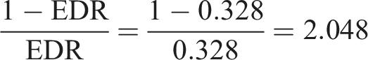
The FDR is 2.048, so we can expect two non-significant UESD ITTs for each statistically significant one. Given that we only observe one non-significant published ITT for each significant published ITT, this suggests that one non-significant ITT is lost in the file drawer for each significant published ITT.

The ERR is the mean unconditional power of a sample of estimates after selection for significance (Bartoš and Schimmack, 2022). It is equivalent to the expected proportion of statistically significant results when conducting an exact replication of the studies behind all statistically significant estimates. To approximate this quantity, z-curves estimate the weighted mean unconditional power of all estimates (weighted by their power). The weights account for the fact that studies with higher power are more likely to produce statistically significant results:

(Notation 5: ERR)

\frac{\sum_{k = 1}^{K} ϵ_{k} \times ϵ_{k}}{\sum_{k = 1}^{K} ϵ_{k}}

The estimated ERR for the sample of statistically significant UESD ITTs is 0.564. If we would conduct exact replications of all statistically significant UESDs in the sample, the expectation maximization algorithm behind the z-curve predicts that 56% of the replicated estimates would be statistically significant. All parameters and their robust bootstrapped 95% confidence intervals are summarized in Table 1. Besides the z-curve reported in this manuscript, I analyze several alternative specifications, including z-curves on cleaned samples, clustered z-curves,¹⁰ and a p-curve in Appendix A2-A6.

Table 1.

Z-Curve estimates and their robust bootstrapped 95% confidence intervals for the full sample of 1095 UESD Z-statistics.

	Estimate	Lower CI	Upper CI
ODR	0.497	0.467	0.527
EDR	0.328	0.123	0.468
FDR	2.048	1.138	7.110
ERR	0.564	0.484	0.659

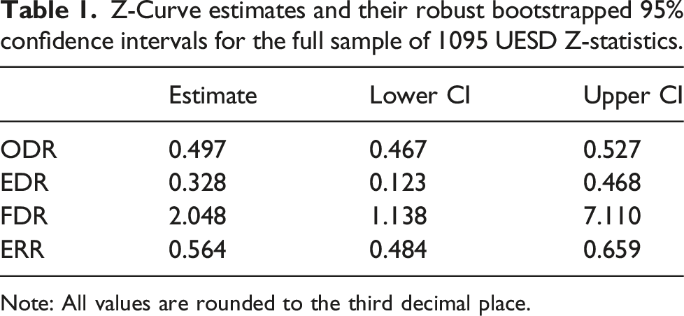
Note: All values are rounded to the third decimal place.

Other approaches to assess publication bias

In the following, I present the results of funnel plots and caliper tests which confirm the presence of anomalous patterns in the distribution of UESD test statistics indicative of publication bias. However, in Appendix A8, I discuss limitations of funnel plots and caliper tests when it comes to the evaluation of publication bias across an entire methodology, such as the UESD, and argue that z-curves circumvent these limitations.

Funnel plots are among the most widely used tools to assess publication bias. The premise of funnel plots is to plot the effect sizes and standard errors of a set of studies against a funnel centered around the mean estimate to determine whether there are any asymmetries in their distribution (Sedgwick 2013). Such asymmetries might then be indicative of publication bias. Two example funnel plots are depicted in Figure 3, where the ITTs and standard errors for two of the most commonly analyzed UESDs are plotted: the effect of terrorist attacks on positive emotions and on anti-immigration attitudes. In both cases there is a slight asymmetry in the funnel plots, with more estimates outside of the funnel tending toward null than estimates outside of the funnel tending toward larger effects. This gives an indication of publication bias toward larger effect sizes than the true mean effect size.

Figure 3.

Funnel plots of two common UESD hypothesis tests. (a) Terrorist Attacks → Positive Emotions (N = 46). (b) Terrorist attacks → Anti-immigration attitudes (N = 39). Note: blue dots are statistically significant estimates (p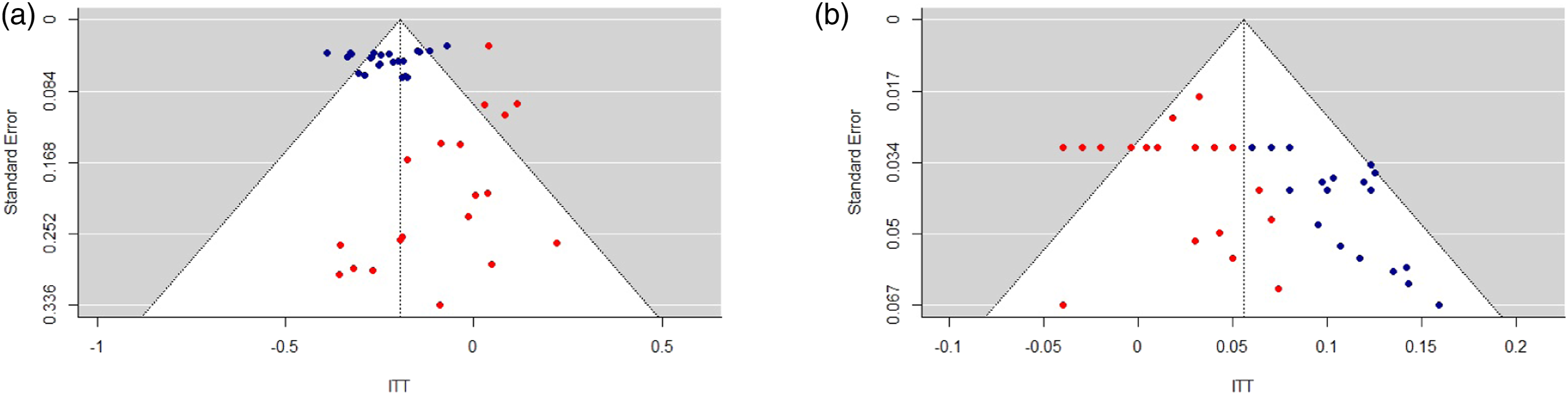 $<$ 0.05); red dots are non-significant estimates.

Caliper tests can also be leveraged to assess publication bias (Gerber and Malhotra, 2013). The premise is simple: within a narrowly defined bandwidth around the significance threshold, the number of statistically significant estimates is compared to the number of non-significant estimates. An abrupt jump around the threshold, leading to a disproportionally high number of significant estimates, indicates publication bias. Table 2 documents four such caliper tests using the full sample of all 1095 UESD estimates.¹¹ In all four cases, the null hypothesis that the jump in estimate quantity around the significance threshold occurs by random chance is rejected, with p-values ranging from 0.00006 to 0.02. This gives another indication of publication bias toward marginally significant results among UESD studies.

Table 2.

Caliper tests of publication bias in all UESD studies.

	Over caliper	Under caliper	p-Value
2.5% Caliper	33	8	0.00006
5% Caliper	46	17	0.0002
10% Caliper	71	42	0.004
15% Caliper	99	70	0.02

Conclusion

This paper presents two important insights: (1) there is a large file drawer of unpublished UESD findings. The expectation maximization algorithm predicts two non-significant findings for each significant one. Empirically, we observe a one-to-one ratio. The file drawer is thus estimated to be equal in size to the number of published statistically significant findings. Considering the upper bound of the confidence interval, it might be up to six times as large. This poses a risk to the credibility of published UESD findings, as they are not representative of the broader universe of discoveries and non-discoveries.

(2) Nonetheless, those UESD findings that are statistically significant and end up getting published are surprisingly replicable. The predicted replication rate of 56% might seem rather low, but it is higher than the rates of many previous large-scale replication attempts in the social sciences. For example, the largest replication effort to date in the social sciences found that only 39% of high-profile psychology findings replicate (Open Science Collaboration 2015).¹²

These results give a mixed impression of the validity of published UESD findings. While most findings seem trustworthy, we now know that many (potentially conflicting) findings have not (yet) made their way into the published literature. UESD practitioners are already fairly open about non-discoveries, with over 550 non-significant ITTs published, but an embrace of precisely estimated null results over imprecisely estimated discoveries would reduce the size of the file drawer substantially. This assessment is strengthened through the analysis of funnel plots and caliper tests, both of which also detect anomalous patterns in the distribution of UESD estimates that are indicative of publication bias.

The z-curve approach can (and should) be used to estimate replicability and the size of the file drawer for other methodologies, including instrumental variables, difference-in-differences, and regression discontinuity designs. Since the literature for these methodologies is more developed than for the UESD, a full-scope review of the entire literature is likely unfeasible, but z-curves could be focused on publications in the top journals. Furthermore, z-curves can be used to estimate replicability and the size of the file drawer for substantial topics or entire subfields in political science.

Supplemental Material

Supplemental Material - Fitting z-curves to estimate the size of the UESD file drawer and the replicability of published findings

Supplemental Material for Fitting z-curves to estimate the size of the UESD file drawer and the replicability of published findings by Joris Frese in Research & Politics.

Footnotes

Declaration of conflicting interests

The author(s) declared no potential conflicts of interest with respect to the research, authorship, and/or publication of this article.

Funding

The author(s) received no financial support for the research, authorship, and/or publication of this article.

Carnegie Corporation of New York Grant

This publication was made possible (in part) by a grant from the Carnegie Corporation of New York. The statements made and views expressed are solely the responsibility of the author.

ORCID iD

Joris Frese

Data availability statement

All replication materials, including data and code, are publicly available at .

Supplemental Material

Supplemental material for this article is available online.

The replication files are available at .

Notes

References

Bartoš

Schimmack

(2022) Z-Curve 2.0: estimating replication and discovery rates. Meta-Psychology 6: 1–14.

Brodeur

Cook

Heyes

(2020) Methods matter: p-hacking and publication bias in causal analysis in economics. The American Economic Review 110(11): 3634–3660.

Brunner

Schimmack

(2020) Estimating population mean power under conditions of heterogeneity and selection for significance. Meta-Psychology 4: 1–22.

Dreber

Johannesson

(2019) Statistical significance and the replication crisis in the social sciences. In: Oxford Research Encyclopedia of Economics and Finance. Oxford, UK: Oxford University Press.

Epifanio

Giani

Icandic

(2023) Wait and see? Public opinion dynamics after terrorist attacks. The Journal of Politics 85(3): 843–859.

Franco

Malhotra

Simonovits

(2014) Publication bias in the social sciences: unlocking the file drawer. Science 345(6203): 1502–1505.

Gerber

Malhotra

(2008) Do statistical reporting standards affect what is published? Publication bias in two leading political science journals. Quarterly Journal of Political Science 3: 313–326.

Gerber

Malhotra

(2013) Publication bias in empirical sociological research - do arbitrary significance levels distort published results? Sociological Methods & Research 37(1): 3–30.

Holman

Merolla

Zechmeister

(2022) The curious case of theresa may and the public that did not rally: gendered reactions to terrorist attacks can cause slumps not bumps. American Political Science Review 116(1): 249–264.

10.

Lee

Scott

(2012) EM algorithms for multivariate Gaussian mixture models with truncated and censored data. Computational Statistics & Data Analysis 56(9): 2816–2829.

11.

McLachlan

Lee

Rathnayake

(2019) Finite mixture models. Annual Review of Statistics and Its Application 6: 355–378.

12.

Muñoz

Falcó-Gimeno

Hernández

(2020) Unexpected event during survey design: promise and pitfalls for causal inference. Political Analysis 28(2): 186–206.

13.

Open Science Collaboration (2015) Estimating the reproducibility of psychological science. Science 349(6251): 1–30.

14.

Ramirez-Ruiz

(2024) The unexpected results of the peace referendum changed conflict termination preferences in Colombia. Research & Politics 11(1): 1–7. doi: 10.1177/20531680241233793

15.

Röseler

(2023) Predicting replication rates with Z-curve: a brief exploratory validation study using the replication database. OSF Working Paper 1–16. doi: 10.17605/OSF.IO/K4D6W

16.

Röseler

Kaiser

Doetsch

, et al. (2024) The replication database: documenting the replicability of psychological science. MetaArXiv DOI: 10.31222/osf.io/me2ub.

17.

Rosenthal

(1979) The file drawer problem and tolerance for null results. Psychological Bulletin 86(3): 638–641.

18.

Sedgwick

(2013) Meta-analyses: how to read a funnel plot. BMJ 346: 1–2.

19.

Singh

Tir

(2023) Threat-inducing violent events exacerbate social desirability bias in survey responses. American Journal of Political Science 67(1): 154–169.

20.

Sterling

Rosenbaum

Weinkam

(1995) Publication decisions revisited: the effect of the outcome of statistical tests on the decision to publish and vice versa. The American Statistician 49(1): 108–112.

21.

Stommes

Aronow

Sävje

(2023) On the reliability of published findings using the regression discontinuity design in political science. Research & Politics 10: 205316802311664. DOI: 10.1177/20531680231166457.

Supplementary Material

Please find the following supplemental material available below.

For Open Access articles published under a Creative Commons License, all supplemental material carries the same license as the article it is associated with.

For non-Open Access articles published, all supplemental material carries a non-exclusive license, and permission requests for re-use of supplemental material or any part of supplemental material shall be sent directly to the copyright owner as specified in the copyright notice associated with the article.

0.00 MB

0.73 MB