
Abstract
The literature surrounding extreme right parties in Europe has developed dramatically over the past two decades. However, the analysis of electoral success for these parties has produced muddled results, and occasionally even conflicting findings. This article argues this confusion is partially due to a reliance on an inappropriate model choice. Through the use of simulations, a goodness-of-fit exercise, and a prediction exercise based on model cross-validation, I show that the traditional Tobit specification—adopted to deal with electoral results of fringe parties—is theoretically untenable, statistically inferior to alternative models, and practically prone to revealing effects that are unsupported by the underlying data. Rather, the results suggest that best practices should see researchers adopt Cragg or Heckman models for two-stage questions, or consider adopting an analysis applying multiple overimputation if the main question is focused on the determinants of electoral success.
Introduction
Although the study of extreme right parties (ERP) in Europe once lagged behind those of other party families, the tide has shifted considerably in the last two decades. Emerging as a politically relevant force in western Europe during the late 1980s and playing an increasingly meaningful role in the post-Soviet countries, ERPs have become the fastest-growing party family in Europe and demanded escalated attention from scholars (Mudde, 2007; Golder, 2016). Of particular interest to academics have been the determinants for ERP electoral success.
The literature is rich with studies attempting to account for electoral support for ERPs across the continent, with possible determinants including increased immigration, historical legacies, and changing economic fundamentals. Establishing an association between any particular determinant and ERP electoral success is challenging, however, given the nature of ERPs.
Due to their extremely targeted appeal and short histories, ERPs tend to be unstable. In many countries, ERPs have risen to a brief moment of prominence, only to disappear in the next election. In some cases, this cycle has occurred more than once. Thus, whereas there may be latent support for extreme-right ideology in a country, there is no guarantee that a particular party will represent those claims in a given election. Vote shares of “zero” are recorded, even if there exists a political environment that would positively support ERPs. This presents a hurdle for researchers attempting to estimate determinants of ERP electoral success. To this point, the literature has tended to address this problem by adopting a Tobit I model specification. This article suggests two possible alternative paths to measuring ERP electoral determinants in cross-national settings, each of which greatly improves on this traditional method.
First, I show that—if researchers want to measure entry and electoral success simultaneously—the assumptions and restrictions of the Tobit I model will produce both inconsistent and inefficient estimates, and alternative methods such as a Cragg-truncated normal hurdle model or Heckman selection model will more appropriately capture the data-generating process. I then further argue that attempting to answer these questions simultaneously leads to reliance on assumptions unlikely to be supported by the data, and that researchers should devote their focus only to estimating determinants of latent electoral support for ERPs. To do so, I suggest a novel way of treating the data problem as a form of measurement error, allowing researchers to use multiple overimputation to generate approximate values for what that electoral support might be under different circumstances. This strips some of the most onerous assumptions of two-step methods away from the problem, and presents a cleaner alternative to scholars studying electoral determinants.
The paper proceeds as follows. The first section briefly characterizes the estimation problem at hand. The next section discusses the use of the Tobit I model to deal with this problem, and proposes Cragg and Heckman specifications as alternative methods for capturing the desired estimates. In the third section, I argue that by addressing the data problem as a form of measurement error, we can use multiple overimputation to better explain the success of participating ERPs. A series of simulations in the fourth section show that all alternatives outperform the traditional Tobit method over a variety of realistic data-generating processes, whereas the fifth section utilizes a prediction exercise based on cross-validation and a goodness-of-fit test to show the alternative model specifications make better and more generalizable predictions. The final section concludes.
The problem with zeros
Previous work in the literature has often noted that an election without ERP competition is not evidence for a lack of support of extreme-right policies. One need only consider as an example Sweden, which contained a variety of local and regional political organizations that expressed ERP-type ideology throughout the late 1960s and 1970s, but would frequently see no contestation at the national level by these parties. Indicative of this trend was the Progress Party, founded to compete nationally but eventually relegated to regional focus in Motala and Stockholm. The zeros we see in national results are misleading because they suggest a lower level of ERP support than actually exists in the country. In any type of naive regression of electoral results on possible determinants, we should expect downward bias in our estimates.
This issue is well known. There are very few examples of articles that fail to account for it or, worse, account for it by removing cases with no participating ERP from the sample. Online Appendix A includes a list of articles that face this difficulty and how they address it. Unfortunately, save for some notable exceptions (see, e.g. Bowyer, 2008a and Coffé et al., 2007) most authors have attributed this issue to a form of data censoring.
This has led authors to account for their zero-replete data by utilizing a Tobit I model, originally discussed in Tobin 1958. However, zeros in this data are not the result of censoring possibly negative results, but from a two-stage process whereby a party first decides whether to enter the competition and then voters choose which competing party to support. 1
Those parties that do not participate will record zeros, whereas those that choose to participate will all record (roughly continuous) positive values of vote share. When we consider the question through this lens, our available analysis options extend beyond the Tobit I.
Model specification in the presence of zeros
There are multiple econometric models to address two-stage problems of this type, of which the Tobit I model is but one example. Not all models are equally effective in all scenarios. This section of the paper discusses the possible models available to researchers, including the Tobit I model relied on in the literature, double-hurdle models and Heckman selection models. Mathematical notation for each method is reserved for Online Appendix B. I briefly discuss contexts in which the assumptions of the model would be most and least appropriate.
Tobit I Model
As discussed above, the Tobit I model is the most commonly adopted model in the ERP literature. It has as a strength its simplicity. So long as its assumptions are met, the estimation via maximum likelihood is straightforward and produces consistent and unbiased estimates for the variables of interest. These assumptions can be very problematic, however.
The most worrisome assumption is that of a single determinative process. 2 The standard Tobit model assumes the same process governs whether an actor participates (the first stage), as well as the level of participation (the second stage, with an observed value). Moreover, this process is fixed, such that the ratio between determinant coefficients is identical in both stages. 3 This is incredibly unlikely to reflect the true situation in the standard case where a researcher is estimating the effect of determinants on ERP electoral support.
Consider, for instance, the number of parties competing in an election. Kselman et al. (2016) have found that as the effective number of parties increases, the likelihood of new party entry increases. However, as the number of parties increases (ceteris paribus), the expected vote share for any one party decreases. In our scenario, we would expect the effective number of parties in a political system will have a positive effect on participation by ERPs, but that actual vote share will decrease in the number of parties, conditional on participation.
This type of opposite impact at the two stages cannot be accurately estimated using the Tobit I model, and the mechanics of the model are such that the specification will produce bias in all covariates while attempting to force the estimated effects into adherence with the assumption. Worse, there is no way of measuring or even predicting the bias. Two alternative two-step method choices, however, relax the assumption of a single determinative process. I cover each briefly below.
Tobit II model
The Tobit II model extends the traditional Tobit model to include two latent variables. Each latent variable is associated with a particular “hurdle”: one governing whether the actor participates, and one the level of participation. Thus, we frequently call these models “double-hurdle” models. When the error terms in each hurdle are uncorrelated, we have the Cragg truncated normal hurdle model (Cragg, 1971), which holds a special usefulness in our situation. However, all forms of double-hurdle model provide a loosening of the restriction concerning a single determinative process.
If we assume independence of the error terms and adopt the Cragg model, we can actually test the alternative Tobit specifications against each other. This is due to the nested nature of the standard Tobit inside the Cragg. We may be loathe to assume independence conditional on the unobservables across both of the processes, so it is appropriate generally to estimate using both a Cragg and full double-hurdle model, which can be compared using a simple log-likelihood test. In this way, we can test the Cragg model against both a standard Tobit model and a full double-hurdle specification.
Heckman selection model
The Heckman model was first created to deal with issues of sample selection (Heckman, 1979). However, it has been used in other fields to effectively model similar problems to the one at hand (see, e.g. Farrell and Walker, 1999 on lottery consumption or Madden, 2008 on alcohol and tobacco use). Its form is extremely similar to the Tobit II model above, but with one critical difference: all zeros are determined at the first stage. That is, once an actor decides to participate, we will observe positive values.
When we observe zeros for ERP vote share, we generally do so because no parties have chosen to participate. Once entered into an electoral competition, no party is likely to receive zero support (presuming minimally that their candidates vote for themselves). Thus, one could argue that the process is of the type that makes the Heckman approach appropriate. Alternatively, an ERP may choose to participate in the election, but be later limited in its ability to gather votes, either due to some actions of their own (failing to meet deadlines, disbanding the party, etc.), actions of others (being removed from the election for some perceived fault) or random occurrences. How researchers choose to model this process may depend on their knowledge of the situation, but it is reasonable to consider a double-hurdle alternative in situations where the exclusion processes occur after the participation decision.
The Heckman model, however, presents some difficulty statistically. Although all parameters can be identified even when the covariates in the first and second part of the process are identical, the estimation can be inefficient. This potential inefficiency is well documented elsewhere (see, e.g. Wooldridge, 2003 and Bushway et al., 2007), so we note here only that the best way to avoid this issue is to include exclusion variables in the participation portion of the equation that are not included in the consumption portion.
Practically, however, this can be very difficult. In our case, it is not immediately clear what types of variables would qualify. Electoral thresholds certainly play a role in the participation decision, but we might also expect that high thresholds may increase strategic voting, and decrease the expected vote share of a participating ERP. Excluding them from the second-stage equation would certainly risk omitted variable bias, replacing inefficiency with inconsistency. Regardless of variable choice, theoretical justifications will need to be strongly convincing. This inherent weakness in the Heckman model should give researchers pause, and force reconsideration of specification selection.
The Cragg and Heckman specifications present two alternatives to the Tobit I model, but face specific difficulties when applied to the facts of the situation. Rather than choosing between known evils, however, researchers might reconsider and re-conceptualize the problem. The next section discusses how one might efficiently and consistently estimate the effects of primary interest by changing the way observed zeros are viewed.
Observed zeros as measurement error: An alternative approach
To this point, researchers have been forced to rely on two-step methods because they are effectively answering two questions: what determines whether an ERP contests an election, and what determines the electoral support for an ERP that does contest an election? However, the latter question seems to be the driving force behind the whole inquiry. 4 If we take this dominance to heart, we might consider instead an analysis plan that focuses only on the associations between contextual covariates and electoral support for ERPs. In this section, I suggest that by considering the recorded zeros as examples of data observed with measurement error and correcting for that error, we can more efficiently address this issue. By doing so, we recognize that the observed zeros give us some information about the underlying latent willingness to support an ERP electorally but not a completely accurate rendering of it.
Traditionally, we perceive measurement error in data as the result of either a systematic or random process connected to the manner of data collection. Generally, one can attempt to intervene in the data-collection process to limit or eliminate the error, or address it post hoc. In this paper, I suggest that we do the latter in a manner consistent with reasonable assumptions about the data-generating process, using multiple overimputation (MO). Online Appendix C discusses MO at greater length, including details on its implementation in the simulations and application below. However, in this section, I briefly discuss the advantages of the process, as well as the necessary assumptions.
MO envisions all data on a spectrum of measurement error, from missing to perfectly captured. All observations can be considered some combination of the “true” latent value and measurement error. This means we can extract at least some information from cell-level data, even when it is observed with known error. In the extreme case, we may treat the zeros as wholly uninformative, overwriting them with purely imputed values. Just as with multiple imputation, the process generates estimates of the latent variable, only it combines the information drawn from the cell-level data with the predicted values from the conditional expectations for the variable. Those estimates can then be used to run our originally intended analysis, giving us both greater consistency and greater efficiency than alternative methods. We also stand on more theoretically satisfying grounds, as the number and strength of our assumptions are reduced.
The primary assumption associated with MO is that of ignorable measurement mechanism assignment (IMMA). IMMA assumes that whether we observe the data in our dataset fully, with measurement error, or not at all, is a function of our observations and random draws from a probability distribution. No unobserved factors can play a role in determining what type of data a particular cell in our dataset is. This is notably a strong assumption, in that we are unlikely to include all appropriate predictors for why an ERP is not challenging a particular election. However, Blackwell et al. (2015) show statistical evidence that IMMA need only minimally hold for MO to produce robust results. In particular, they show that even with imperfect or incomplete proxies for the latent variable or predictors for measurement error, bias in the covariates is minimal. 5 This is true even when measurement error is correlated with both the observed outcome and the true latent value, both of which are true in our case. 6 It is also important to note that because the variable being overimputed in this scenario is the dependent variable in our analysis, any bias in the imputation will serve only to make our estimates less efficient, not to introduce bias in our estimated coefficients.
As best practices, they suggest including not only all predictors that will be included in the model, but all possible predictors of the latent variable, as well as all potential predictors of being measured with error, and possibly important nonlinearities among all of these. In our case, the first and second should be roughly the same (as the variable we are measuring with error is also the outcome variable of the model), but the third could include variables such as whether the country saw an ERP contesting the previous election, or even the mean cross-national likelihood of an ERP contesting an election in that era. We might finally also note that, although IMMA can still seem onerous, there are similar implicit assumptions in the two-stage methods, where under-specification of either stage will introduce bias to our estimates (via omitted variables), and in the case of the Tobit I model, will diffuse that bias across both stages.
Using MO to conduct our analysis yields a few advantages over the two-step methods. First and foremost, MO allows researchers to treat observed zeros differentially, impossible in two-step models. The lack of ERP participation in an election may stem from multiple causes, from the scenario where no ERP exists in the country to one where a previously successful ERP either collapses mid-cycle, or is expelled from competition. 7 If the researcher can include the relevant predictors of underlying support, 8 the imputation process should produce latent estimates for electoral support that are closer to the true potential electoral support, and a model run on the combination of the imputed latents and observed positive values will be more predictive and accurate than models that are trained on only observed positive values.
As a related secondary advantage, we can now use all of the observations in our sample to estimate the effects of the desired determinants of electoral support, rather than only those observations with observed positive values. Given how many zeros we generally face in these analyses, this increases efficiency dramatically, even after accounting for the uncertainty attached to the imputed datasets. Our estimates have the potential to be more precise, and the reduction in noise may lead to better identification of substantively important associations in our data.
The next two sections demonstrate the practical impact of model choice in our situation, displaying the weakness of the standard Tobit I model and confirming the strength of our alternative methods.
Model performance in the presence of zeros: A simulation
We start with a simulation exercise for general applicability. The simulations assume knowledge of an underlying data-generating process, and then proceed to test each model’s ability to accurately capture that process. The simulations are naturally a simplified version of reality (where the data-generating process is unknown), but it helps to set an even playing field for the models, as well as establish a metric for performance. I discuss the assumptions of the simulation below, before continuing with the results.
I constructed eight simulations of the same basic pattern. 9 Three covariates control both a first and second stage, in a known process with random noise. All four specifications are used to model the data and each model is gauged based both on accuracy and efficiency. The eight simulations vary on several dimensions.
First, I vary the degree to which the three covariates control each stage “similarly,” which is when the covariates provide proportional effects in both stages. Perfectly proportionate effects across both equations and all three covariates would most favor the traditional Tobit I model, as an assumption of a single determinative process is not unfounded.
I also vary the likelihood of participation and thus, the number of zeros observed in the simulated dataset. I set three different levels for observed zeros, one lower than is traditionally observed in the literature, one right at the median, and a level higher than most commonly observed. Each of these levels is interacted with a level of “similarity” that is either high or low to produce six simulations.
The seventh simulation allows for what I term “ejection.” In this simulation, some observations that meet the participation threshold are still registered as zeros, based on their level of a fourth, unmodeled covariate. These observations are meant to simulate situations in which ERPs may desire to participate, but are stopped by forces outside of their control. This simulation highlights a particular weakness in the Tobit model, as increasing the unpredictability of the participation portion of the equation bleeds into the estimation of the second-stage covariates. In the final simulation, I allow for correlation in the error terms in the two equations. Primarily, this eighth simulation is to test the robustness of the Cragg model. As described above, the Cragg model relies on the assumption of uncorrelated error terms between the two processes, but how greatly the estimation suffers given correlation is unknown.
Table 1 shows the results of all eight simulations. It should be noted that the Tobit I model performs worst in all of the simulations. This includes the “friendliest” situation: the simulation with the tightest proportionality between the two processes, the least randomness in generating zeros and the least zeros overall (Simulation 3).
Simulation results.

The table displays the results of eight simulations testing four different models. The simulations are briefly described in the left column, with the mean number of zeros reported in the second column. Columns 5–8 report the RMSE in estimating the coefficient attached to a particular covariate for each model specification. The results in bold indicate the model whose RMSE was the smallest for the particular covariate estimate.
MO: multiple overimputation; OLS: ordinary least squares; RMSE: root mean square error.
The final four columns of Table 1 report the root mean square error (RMSE) attached to each specification choice, broken down by covariate. These numbers present (approximately) how much error we would expect in the estimated coefficients (whose true values are recorded in the column to the left of these results). Two things stand out. First, the Tobit model does extremely poorly in comparison to all three alternatives, its RMSE routinely three to seven times larger than the other models. This is true across all the simulations. Note that larger error in the estimates will produce more spurious inferences.
Looking at the bold results (which present the lowest error for that covariate), we can also see the Cragg method outperforms the Heckman model between the two-step models, whereas the results for the Cragg model and the model utilizing multiple overimputation perform extremely similarly. This latter accords with our expectation as the estimation strategies underlying the two are nearly identical (a truncated linear regression versus ordinary least squares) on slightly different samples. 10
The simulations suggest that, statistically, the alternatives to the Tobit I model presented in the previous section should all be preferred, even in situations that we believe are governed by the data-generating process most friendly to the Tobit model. In the next section, I show the practical effects of relying on the Tobit model over superior models.
Effects of model choice
The simulations speak to the statistical superiority of our alternative models, but one might ask what the practical effect of poor model choice actually is. In this section, we use an existing analysis, based on strong theoretical arguments, to conduct both a prediction and a goodness-of-fit exercise, each measuring the extent to which different models fit the underlying data and could be used to predict vote share for an ERP.
Prediction exercise
An often implicit assumption of modeling is that the resultant model could be used to predict levels of the dependent variable in unobserved situations. This assumption speaks to the generalizability of the model outside of the sample used. Thus, one way of judging model choice is to compare the ability of alternative specifications to predict out-of-sample observations. Those models that come closest to predicting observed levels of the dependent variable should be considered more reliable.
I conduct such a prediction exercise here. To ensure the test properly adjudicates between the various functional forms, I use one model, adapted for each of the specification choices discussed in the paper. By holding constant the variable choice within the specification, I ensure that I am isolating prediction differences on functional form alone. For this exercise, I adopt the data and model used in Golder (2003). Although I explain this choice in greater depth in Online Appendix G, 11 the major advantages include the model’s simplicity, the availability of the data, and that the approach is broadly representative of the ERP literature. In addition, using a pre-developed model restricts my discretion in testing the functional forms against each other.
The exercise is constructed as one of an exhaustive cross-validation. Using the sample of data provided by Golder,
12
I remove one observation from the dataset to use as a test, and train the model on all remaining (
The table displays the results of a prediction exercise testing four different specifications. Columns 2 and 3 report the root mean square error and mean absolute error (MAE) of the specification, using the entire sample. Columns 4 and 5 report the same measures only on the observations in the sample where an extreme party participated. The best performances are bolded.
Table 2 displays the results of the prediction exercise for each of four different functional forms. Error is measured using both RMSE and the MAE. I compare model-predictive performance in two ways. First, in columns 2 and 3, I compare how well each model predicts all observations in our sample. This is an appropriate test if a researcher is interested in predicting vote share for ERPs in a country, but has no additional knowledge if such a party is likely to compete in an election. In columns 4 and 5, I report measures of the model’s accuracy for the subset of observations where ERPs actually contested the election. This is an appropriate test if the researcher is attempting to predict support for an ERP in a country that is known to be competing. 13
Prediction exercise results.

MAE: mean absolute error; MO: multiple overimputation; OLS: ordinary least squares; RMSE: root mean square error.
The results are as expected. When researchers know only about past results, the two-stage models better predict all observations, with the Cragg outperforming both the Heckman and Tobit models within that subgroup. However, the model utilizing MO better predicts non-zero observations. In both tests, the gains in accuracy are meaningfully large, with the Cragg outperforming the second-place Tobit by 6.3% and 8.5% in RMSE and MAE, respectively, and MO+OLS reducing error in non-zero observations over the second best method (the Heckman model) by 10.1% (RMSE) and 2.0% (MAE), and the Tobit model by 18.0% and 4.3%. Overall, the prediction exercise confirms the arguments above: choice of functional form depends on the questions being asked, but there remain better alternatives to the traditional Tobit approach regardless of what those questions may be.
Goodness-of-fit exercise
One could alternatively conduct a goodness-of-fit exercise to judge how much information a particular model choice allows us to capture from the data, as well as the quality of the inferences we can draw. I do so here, replicating Golder (2003) using the model alternatives. The replication is fully described in Online Appendix G, but for the purposes of this exercise I focus on model fit and the inferences we might potentially draw from alternate model choice.
The table displays the estimates of the effects of covariates on ERP vote share, given that an ERP participates. The first column represents the effect as estimated by an OLS+fixed effects specification, with vote shares imputed for units observed with zero support. The second column represents the effects estimated in the second stage of a Heckman model, whereas the third column presents the estimates from the second stage of a Cragg model. The final column presents the estimates derived from the panel-adjusted Tobit model.
Table 3 displays the coefficients attached to each model, and particularly the second-stage coefficient estimates for the two-stage models. One might draw very similar inferences from all four models, save for one covariate. An increase in the percentage of seats allocated above the district level is associated with higher vote share for ERPs. 14 The interaction between unemployment and immigration levels also seems to be positively associated with increased electoral support, although it is imprecisely measured in two of the models. However, the main finding of the Tobit model used in the original piece, that higher levels of immigration are associated with higher ERP vote share all else equal, is not supported in the remaining three models.
Estimates for covariate effect on ERP vote share, conditional on participation.
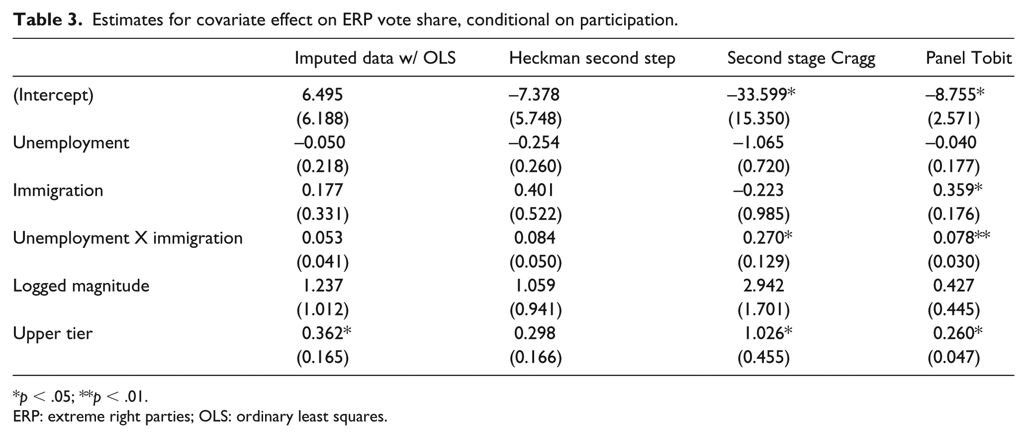
p < .05; **p < .01.
ERP: extreme right parties; OLS: ordinary least squares.
We can use goodness-of-fit statistics to adjudicate between three of our competing models. As mentioned above, the Tobit I model is nested inside the Cragg, which allows for the use of a simple likelihood ratio (LR) test. The LR test has as its null that the smaller, more restrictive model (here, the Tobit) is the better fit. In this analysis, comparison yields a test statistic of 155.29 (distributed Chi-square) with 19 degrees of freedom. The resulting p value strongly favors rejection of the null and supports the notion that the Cragg double hurdle model is the superior choice in this case.
As between the two-stage models, the case is less clear. The models are non-nested, necessitating the use of a Vuong test. 15 Here, the null is that the models are equally close to the true data-generating process, and when we compare the Cragg and Heckman models, we generate a Vuong statistic of -1.003, which does not allow us to reject the null that the models capture the data-generating process equally well.
In general, however, our goodness-of-fit exercise supports the case made in the prediction and simulation exercises, and shows how suboptimal model choice can lead to incorrect inferences.
Conclusions
This article stresses the importance of carefully considering model choice when analyzing data replete with “zero cases.” I argue that the traditional method used to study electoral determinants of fringe parties is suboptimal, with negative consequences for our continued quest for understanding.
Three final considerations should be addressed. First, although I advocate for the use of multiple overimputation and a single analysis in this article, it should be clear to readers that both the double-hurdle and Heckman models can be appropriate choices depending on the assumptions that one is willing to make and the questions one seeks to answer.
Second, model choice is but one issue in the study of ERP electoral support. Although this piece concentrates almost solely on that choice, researchers should be cognizant of additional issues. It is not entirely clear, for instance, that cross-national research in this area is the ideal structure of analysis. Bowyer makes a particularly valid point in this vein (Bowyer, 2008b), demonstrating that ERPs in many countries may choose to participate in national elections selectively at the district or local level. In this case, the parties are only “partial” participators and our observed non-zero vote shares may still be underestimates. To appropriately model this factual situation, the researcher should dig down to the lowest level at which zeros are created, and analyze from there. This level of detail suggests that within-country studies may be more tenable, if only because of the sheer enormity of the task of measuring thousands of districts across countries and time.
Finally, although this paper has focused on the study of ERPs in Europe, the methodological issues discussed here may impact different lines of study. Quite naturally, studies of any fringe party, including the far left, will face similar concerns over the underestimation of electoral support. Opposition or anti-establishment parties in one-party states may face similar challenges to ERPs in terms of entering the electoral fray. In that case, we might mistakenly understate the support for opposition if we consider non-existent electoral returns as “true” zeroes.
Similarly, an ERP’s failure to compete in a national election is only one way latent support for smaller parties goes underestimated. Strategic voting due to high electoral thresholds or expected exclusion from parliament or coalitions can also yield similar methodological concerns, and the application of an overimputation scheme akin to the one described in this article may be worthwhile in studies of party support and parliamentary composition more generally. Future research into each of these areas should be explored.
Computer packages used
Henningsen, Arne and Toomet, Ott (2011) maxLik: A package for maximum likelihood estimation in R. Computational Statistics 26(3), 443–458.
Hlavac, Marek (2015). stargazer: Well-Formatted Regression and Summary Statistics Tables. R package version 5.2. http://CRAN.R-project.org/package=stargazer
Imai, Kosuke, Gary King, and Olivia Lau. Toward A Common Framework for Statistical Analysis and Development. Journal of Computational and Graphical Statistics. Vol. 17, No. 4 (December 2008): 892–913.
Supplemental Material
RandP_Final_Version_-_Appendices – Supplemental material for Much ado about nothing: Zeros and the extreme right
Supplemental material, RandP_Final_Version_-_Appendices for Much ado about nothing: Zeros and the extreme right by Sean Kates in Research & Politics
Footnotes
Acknowledgements
The author would like to thank Neal Beck, Matt Golder, Pablo Querubin, Arturas Rozenas, Arthur Spirling, and Joshua Tucker for insightful comments on earlier versions of this article, as well as the editorial team and reviewers for greatly improving the piece. Any remaining errors are those of the author.
Declaration of conflicting interest
The author(s) declared no potential conflicts of interest with respect to the research, authorship, and/or publication of this article.
Funding
The author(s) received no financial support for the research, authorship, and/or publication of this article.
Supplemental materials
Notes
Carnegie Corporation of New York Grant
This publication was made possible (in part) by a grant from the Carnegie Corporation of New York. The statements made and views expressed are solely the responsibility of the author.
References
Supplementary Material
Please find the following supplemental material available below.
For Open Access articles published under a Creative Commons License, all supplemental material carries the same license as the article it is associated with.
For non-Open Access articles published, all supplemental material carries a non-exclusive license, and permission requests for re-use of supplemental material or any part of supplemental material shall be sent directly to the copyright owner as specified in the copyright notice associated with the article.