Sage Journals: Discover world-class research

Abstract

Enns et al. respond to recent work by Grant and Lebo and Lebo and Grant that raises a number of concerns with political scientists’ use of the general error correction model (GECM). While agreeing with the particular rules one should apply when using unit root data in the GECM, Enns et al. still advocate procedures that will lead researchers astray. Most especially, they fail to recognize the difficulty in interpreting the GECM’s “error correction coefficient.” Without being certain of the univariate properties of one’s data it is extremely difficult (or perhaps impossible) to know whether or not cointegration exists and error correction is occurring. We demonstrate the crucial differences for the GECM between having evidence of a unit root (from Dickey–Fuller tests) versus actually having a unit root. Looking at simulations and two applied examples we show how overblown findings of error correction await the uncareful researcher.

Keywords

Time series error correction equilibrium

Introduction

In a recent symposium in Political Analysis Grant and Lebo (2016) and Lebo and Grant (2016) raise a number of concerns with use of the general error correction model (GECM). In response, Enns et al. (2016) have contributed “Don’t jettison the general error correction model just yet: A practical guide to avoiding spurious regression with the GECM.” Enns et al. are prolific users of the GECM; separately or in combination they have authored 18 publications that rely on the model, often relying on significant error correction coefficients to claim close relationships between political variables. In “Don’t jettison…” the authors narrow the gap of disagreement between themselves and Grant and Lebo. However, as they attempt to reconcile old findings with new insights, Enns et al. inadvertently make clear an essential point: using the GECM is more complicated in practice than researchers realize. Despite their extensive experience, Enns et al. are still misinterpreting the inferences provided by the error correction coefficient and as a result are overstating relationships between variables.

In this paper we explain where we agree with and diverge from Enns et al.. In short, there is agreement that: (a) with stationary data (I(0)) the GECM’s parameters have different meaning and the strong possibility of user error makes the model a poor choice; and (b) the GECM is more easily interpretable with all unit root (I(1)) and jointly cointegrated data so long as one uses the correct critical values. Many disagreements remain. In particular, despite the weaknesses of the Dickey and Fuller (1979) stationarity test, Enns et al. treat the test’s results as perfectly reliable for identifying unit roots. We show both the high frequency of the Dickey–Fuller (DF) test misclassifying series as unit roots and the consequences for using such series in the GECM. Further, Enns et al. advocate stretching the use of “unit root rules” into other data scenarios but ignore the possible consequences of doing so.

We also explore differences in our understanding of the data used in Kelly and Enns (2010) and Casillas et al. (2011). Enns et al. argue that the data and analyses in those papers and potentially many others fit neatly into the unit root rules category. We maintain that Enns et al. are likely misclassifying the series in those papers as unit roots which can lead to over-stated claims of error correction. We begin with the points of agreement between Enns et al. (2016) and Grant and Lebo (2016).

Points of agreement

The GECM can work when all the series contain unit roots and are jointly cointegrated

The GECM has several representations but the one most commonly used by political scientists is DeBoef and Keele’s (2008) Equation 5:

Δ Y_{t} = α_{0} + α_{1}^{*} Y_{t - 1} + β_{0}^{*} Δ X_{t} + β_{1}^{*} X_{t - 1} + ϵ_{t}

(1)

Enns et al. and Grant and Lebo agree with the literature in econometrics that when both $X$ and $Y$ contain unit roots – defined as $y_{t}$ = $1 * y_{t - 1}$ + $ϵ_{t}$ – and are cointegrated, the combination of $Y_{t - 1}$ and $X_{t - 1}$ is stationary and the equation is balanced. In such cases Equation 1 has acceptable Type I error rates for all its parameters and is readily interpretable.

In particular, there is agreement that when both $X$ and $Y$ contain unit roots:

functions as a test of cointegration between $X$ and Y and measures the rate of error correction, theoretically bounded between 0 and -1.

The critical values for ${\hat{α}}_{1}^{*}$ are non-standard, more negative than with the normal distribution, vary with the number of $X$ s, vary with the length of the data, and can be calculated as “MacKinnon values” following Ericsson and MacKinnon (2002).

When ${\hat{α}}_{1}^{*}$ ’s $t$ -statistic does not surpass the MacKinnon critical value (CV) there is no cointegration. Since $Y_{t - 1}$ and $X_{t - 1}$ are not in combination stationary there is unresolved autocorrelation on the right-hand-side and the model’s estimates should not be used.

This is progress. Grant and Lebo (2016) point out in their table 2 how frequently a researcher might mistakenly conclude error correction is present if she were to incorrectly use the normal distribution to evaluate $α_{1}^{*}$ with unit root series. Enns et al. recognize this when they say: “Thus, the bottom row of Grant and Lebo’s Table 2 should be read as evidence of the importance of using the correct MacKinnon critical values when testing for cointegration, not evidence of spurious relationships with the GECM” (Enns et al., 2016: 3). To be sure, Grant and Lebo’s table 2 is one of many of their analyses intended to demonstrate what happens if – as Kelly and Enns (2010) and Casillas et al. (2011) do – one uses common but incorrect practices.¹

The GECM is possible but not recommended when all series are stationary

Enns et al. and Grant and Lebo agree on another key point: the GECM must be interpreted differently when all the data are stationary compared to when they all contain unit roots.

DeBoef and Keele (2008) and Keele et al. (2016) explain the equivalence of the GECM (Equation 1 above) to the autoregressive distributed lag (ADL) (Equation 2):

Y_{t} = α_{0} + α_{1} Y_{t - 1} + β_{0} X_{t} + β_{1} X_{t - 1} + ϵ_{t} .

(2)

Stationary series require the “stationary rules” for Equation 1: (1) $α_{1}^{*}$ does not test cointegration; (2) $Y_{t - 1}$ ’s hypothesis test evaluates ${\hat{α}}_{1}^{*} + 1$ and MacKinnon CVs are not used (Bannerjee et al., 1993: 167); and (3) estimates must be translated to the ADL framework as $α_{1}^{*} + 1 = α_{1}$ , $β_{0}^{*} = β_{0}$ , and $β_{1}^{*} = β_{0} + β_{1}$ . Thus, when ${\hat{α}}_{1}^{*} = - 1.00$ with a $(0, 0, 0)$ series it indicates stationarity – no impact of $Y_{t - 1}$ on $Y_{t}$ in the ADL.

We did not find these post-estimation calculations in any of our selected readings of the roughly 500 papers that cite DeBoef and Keele (2008). Instead, when data are claimed to be stationary, the value and significance of ${\hat{α}}_{1}^{*}$ and ${\hat{β}}_{1}^{*}$ are taken from software output and treated the same as they would be using the unit root rules. Typically, this leads to overconfidence in rejecting null hypotheses and in finding error correction to be occurring.

Thus, Grant and Lebo do not say that the GECM cannot be used with stationary data, but argue (Grant and Lebo, 2016: 4): “…although the autoregressive distributed lag (ADL) model is algebraically equivalent to the GECM, the reorganization of parameters is not benign and easily leads to misinterpretation.” In other work Kelly, Enns, and Wohlfarth did not adapt their interpretation of the GECM while arguing data are stationary but, with “Don’t Jettison the GECM Just Yet,” the authors are now on board, saying (EKMW, p. 6): “Thus, we agree with Grant and Lebo that when the dependent variable is stationary, the parameterization of the GECM is more likely than the ADL to lead to errors of interpretation.”

This is also progress. DeBoef and Keele (2008) advocate the GECM with stationary data – an early version of the paper was entitled “Not Just for Cointegration: Error Correction Models with Stationary Data.”² With all stationary series, they argue, one can estimate an error correction model (ECM) without discussing cointegration, long-run equilibria, or error correction rates. However, in addition to interpretation problems, other issues followed as well.

A key misreading of DeBoef and Keele is to conclude that the GECM is perfectly flexible so that series of any type can be analyzed together within it.³ In particular, DeBoef and Keele’s (2008: 199) statement that “…as the ECM is useful for stationary and integrated data alike, analysts need not enter debates about unit roots and cointegration to discuss long-run equilibria and rates of reequilibration” has been repeatedly quoted but seldom understood.⁴ The applied literature is peppered with statements such as: “In summary, the ECM is a very general model that is easy to implement and estimate, does not impose assumptions about cointegration, and can be applied to both stationary and nonstationary data” (Volscho and Kelly, 2012); “The ECM provides a conservative empirical test of our argument and a general model that is appropriate with both stationary and nonstationary data” (Casillas et al., 2011); and “While the use of an ECM is often motivated by the presence of a nonstationary time-series as a dependent variable, our application of this model is based on the fact that it is among the most general time-series models that imposes the fewest restrictions” (Kelly and Enns, 2010). Engle and Granger’s (1987) strict rules for cointegration were increasingly ignored as the GECM became the dominant technique in political science.

Enns et al.’s conclusion that “Although the ADL and GECM produce the same information (in different formats), the ADL is less likely to yield errors of interpretation when $Y$ is stationary” (Enns et al., 2016: 10) matches Grant and Lebo: “…with stationary data, the ADL and GECM may be mathematically equivalent but the GECM adds complications without adding useful insights” (Grant and Lebo, 2016: 27). For example, Casillas et al. (2011) use the obviously stationary series Salient Reviews in the GECM and report an error correction rate of 126%, precisely the kind of misinterpretation the ADL can avoid. Thus, while all agree on the mathematical facts, from a practical standpoint Enns et al. and Grant and Lebo are on one side of the issue – recommending against using the GECM with stationary data – and DeBoef and Keele are on the other.

Point of likely disagreement

On another point agreement is uncertain. Grant and Lebo posit that the univariate properties of all series in the GECM deserve attention; for example if all the independent variables are I(1) they must all be cointegrated with the dependent variable (DV). As opposed to Engle and Granger’s (1987) two-step ECM or Clarke and Lebo’s (2003) three-step fractional ECM, the GECM does not allow testing for cointegration or measuring error correction between $Y$ and a subset of $X$ s.⁵

For example, the cointegration of unit root series $Y$ and $X$ in Equation 1 makes the component $(Y_{t - 1}$ + $X_{t - 1})$ jointly stationary and, along with ∆ $Y_{t}$ and ∆ $X_{t}$ , all components will then be stationary and inferences can be carefully drawn. Adding an I(1) $X_{2}$ means adding two predictors, ∆ $X_{2, t}$ and $X_{2, t - 1}$ but if $X_{2}$ is not jointly cointegrated with $Y$ and $X$ the model creates problems due to unresolved autocorrelation in $X_{2, t - 1}$ . Thus, even if cointegration exists between $Y$ and $X$ , researchers need to be more concerned about the properties of other $X$ s. Enns et al. (2016: 9) do not seem worried, for example, defending Casillas et al.’s (2011) table 1 and table 2 (model 1) even though both include a Social Forces variable that is not significant in either lags or differences.⁶ More generally, the consequences of additional non-stationary $X$ s that are not cointegrated are not well understood but are often included in GECM applications. Next we turn to areas of more explicit disagreement.

Points of disagreement

To review, all agree that a bivariate GECM estimates parameters $α_{0}$ , $α_{1}^{*}$ , $β_{0}^{*}$ , and $β_{1}^{*}$ and that with unit root data we evaluate each “as is” but use MacKinnon CVs (Ericsson and MacKinnon, 2002) for the ECM parameter, $α_{1}^{*}$ . Also, with stationary data we need to switch the rules: $β_{1}^{*} = β_{0} + β_{1}$ of the ADL, $α_{1}^{*}$ is not a cointegration test, and $α_{1}^{*} + 1$ relies on the $t$ -distribution.

Our views deviate as we confront the stark choice about which rules to apply, especially with respect to the error correction coefficient. When should we switch from one set of rules to the other? Enns et al. claim that it is possible to unambiguously choose rules based on results from augmented Dickey–Fuller (ADF) tests: “If the ADF rejects the null of a unit root, we do not use the GECM to test for cointegration” (Enns et al., 2016: 4).

However, DF tests have a null hypothesis of a unit root so that positive evidence is required to classify the series as not I(1). As Enns et al. (2016: 4) admit “it is well known that ADF tests are underpowered against the alternative hypothesis of stationarity” meaning that many series incorrectly show evidence of a unit root. Indeed, the ADF test is sensitive to sample size, trends, and bounds. Fractionally integrated, near-integrated, autoregressive, and other stationary series often fail to reject the null in the ADF test. ADF tests can also be affected by trending, periodicity, and heteroskedasticity.

Falsely classifying series as I(1) means being too quick to favor the GECM over the ADL, to apply the wrong rules to the GECM, and to think that lower values of $α_{1}^{*}$ indicate error correction between series and not simply the stationary tendencies of $Y$ .

Figures 1(a), 1(b), and 1(c) show these problems for the GECM. We generated 60,000 pairs of unrelated time series – 10,000 each for T = 50, T = 100, and T = 250 while varying $ρ$ and then again while varying $d$ . Figure 1(a) shows, for each T, 1,000 pairs of simulated autoregressive ( $ρ$ ) series for each of ( $0, 0, 0$ ) to ( $0.9, 0, 0$ ) in increments of 0.1. Figure 1(b) shows 1,000 pairs of fractionally integrated series simulated as ( $0, 0, 0$ ) up to ( $0, 0.9, 0$ ) increasing $d$ in increments of 0.1. Thus, none of these series contain a unit root.⁷

Figure 1.

(a) With $ρ < 1$ , augmented Dickey–Fuller false negatives are rampant and occur with downward biased $α_{1}^{*}$ .

For both Figures 1(a) and 1(b), each shape shows the average value of 1,000 ADF test statistics of $Y$ with vertical whiskers showing coverage of 950 of the 1,000 statistics. The horizontal line is the 0.05-level CV above which are false negatives – a failure to reject the I(1) null with data that are not I(1). The many instances above the line indicate that the test is drastically underpowered.⁸

On the $X$ -axis is the average estimated ${\hat{α}}_{1}^{*}$ from the GECM. As $ρ$ or $d$ moves away from I(1) the ECM value drops lower, seemingly – but not actually – indicating error correction.

The figures’ results should be striking, most especially for short time series. Unrelated series simulated as $(0, 0.5, 0)$ with T = 50 have an average ECM value of -0.53 while failing to reject the ADF null 61.1% of the time. Series that are $(0.5, 0, 0)$ with T = 50 have an average ECM value of -0.56 but appear to be unit roots in the DF test 36.9% of the time.⁹ When $d = 0.8$ and T = 50 – about where many yearly public opinion series fall – the ADF test has false negatives at a rate of 76.1%. In these cases we would find an average ECM of -0.26 and be well on our way to touting error correction. With longer series there are still problems.

Of course, the high rate of false negatives on the ADF test would not be as problematic if the ECM parameter testing for cointegration $(α_{1}^{*})$ did not reach statistical significance. Proponents of the GECM like Enns et al. might suggest that using MacKinnon CVs for the ECM parameter would prevent us from finding false evidence of cointegration in such a scenario. Unfortunately, MacKinnon CVs are not a panacea here, since they rely on the assumption of unit root data and are not extreme enough to prevent falsely finding error correction when series are not unit roots.

Figure 1(c) shows this. Each cell reports the proportion of times that the ADF test fails to reject a false null hypothesis of a unit root and the ECM parameter is significant beyond MacKinnon CVs. For example, with series created as $(0.6, 0, 0)$ and T = 50 there is a 29.9% chance of concluding both that $Y$ has a unit root and that it is cointegrated with $X$ . With series created as $(0, 0.6, 0)$ and T = 100 the rate is 43.4% for finding cointegration when following the exact procedures that Enns et al. advocate. The problems are noticeably more pronounced with data we create as fractionally integrated compared to autoregressive. Additionally, shorter time series are much more problematic – at T = 250 the problems remain for fractionally integrated series with higher values of $d$ but disappear when there is only autoregression and the ADF test is more powerful.

To reiterate, not a single series in Figures 1(a), 1(b), or 1(c) contains a unit root. Thus, the GECM’s unit root rules should not be used for any of them.¹⁰ Still, Enns et al.’s favored ADF test will incorrectly conclude that many are I(1). In fact, with short series the ADF test gives us false negatives a majority of the time and even 15% of the time when series are complete white noise, that is, $(0, 0, 0)$ . Nevertheless, Enns et al. would advise applying the unit root rules and MacKinnon CVs to those ADF false negatives without realizing that much of the apparent error correction – see ${\hat{α}}_{1}^{*}$ decreasing from right to left – is due to the distance the series is from actually being I(1).¹¹ In all, the figures show how easy it is to have faulty evidence of both a unit root and error correction.

Enns et al. do not confront these problems. Instead, they force non-unit root data into the “all unit root” case and rely on the error correction parameter $(α_{1}^{*})$ for key inferences. Enns et al. interpret the GECM’s results in the same way whether their series have “evidence of a unit root” or are actually simulated as unit roots.¹² In reality, data are messy and many non-unit root series will provide evidence of being I(1). So, yes, understanding $α_{1}^{*}$ with data simulated to be exact unit roots is straightforward but this does not mean we can reliably interpret the coefficient when using real world time series with unknowable properties.

If we could identify with certainty I(1) series we could know when to apply the unit root rules but, as Enns et al. correctly point out, “It may be that with short time series, we cannot draw firm conclusions about the time series properties of variables” (Enns et al., 2016: 9). Given that, Enns et al. should not choose rules based on a weak test and should not focus on a parameter whose interpretability gets muddier as data deviate from exactly I(1). Doing so gambles with inferences since if the data are not truly I(1) then $α_{1}^{*}$ does not mean what they think it means.

Elsewhere, Enns et al. are explicit about extending the unit root rules to data that are not I(1). In their Case 4, Enns et al. apply them to near-integrated data – where $ρ$ is close to but not equal to one in $y_{t}$ = $ρ * y_{t - 1}$ + $ϵ_{t}$ .¹³ Such series may provide evidence of a unit root but are technically mean stationary. How do we choose which set of rules to use? Banerjee et al. say in the context of ECMs: “In finite samples the differences between, for example, an AR(1) with parameter 1.0 and an AR(1) with parameter 0.99 is a difference of degree rather than kind” (Banerjee et al., 1993: 225). So perhaps we should not switch rules when $ρ = 0.99$ just because the series is technically stationary.

But the unit root rules are not exactly correct when $ρ = 0.99$ either. As Figures 1(a), 1(b), and Grant and Lebo’s (2016) table 4 show, as data move away from unit roots there is a steady progression from 0 to -1 in the estimation of ${\hat{α}}_{1}^{*}$ . This means that the correct critical values are even more extreme than MacKinnon’s values. We could derive correct idiosyncratic CVsc if we could simulate data with the exact same properties but this is a practical impossibility.

Thus, when do we switch from one set of rules to the other? There is no magic threshold as a series goes from $ρ = 1.00$ to $ρ = 0.99$ or from $ρ = 0.90$ to $ρ = 0.89$ where on one side $α_{1}^{*}$ is a cointegration test and the error correction rate and on the other side it is neither. At some point an ADF test statistic will tip from non-significant to significant but this cannot tell us the extent to which $α_{1}^{*}$ speaks to error correction. Using more extreme MacKinnon CVs prevents many false positives in Enns et al.’s simulation exercises but it does not mean they are correct when data are not unit roots.¹⁴

Enns et al. oversimplify again when they use unit root rules for fractionally integrated (FI) series where $0 < d < 1 .$ ¹⁵ Unsurprisingly, they find that many spurious results can be avoided by applying MacKinnon CVs to Grant and Lebo’s (2016) FI simulations and they say: “Again we find, however, that the different conclusions can be resolved by following Grant and Lebo’s advice to test for cointegration with the correct critical values” (Enns et al., 2016: 7).

This seems disingenuous. Neither Grant and Lebo (2016), Ericsson and MacKinnon (2002), nor any other source we know of has argued that MacKinnon CVs are appropriate except with exact I(1) data. Enns et al. provide no justification for expanding when these values should be used – to NI data, FI data, or any other type. Yes, Enns et al.’s advice prevents some spurious findings but that does not mean that these are the correct critical values. As Grant and Lebo’s (2016) figure 4 shows, $α_{1}^{*}$ ’s distribution quickly gets even more extreme than MacKinnon’s distribution as $d$ decreases from 1. Unless we simulate data ourselves, we cannot be sure of the exact $(p, d, q)$ models which means we cannot calculate exactly what the idiosyncratic CVs are. Grant and Lebo point out that “Even if we could pin down the correct critical values, the meaning of the ECM coefficient has been lost. Ultimately, the value of $α_{1}$ tells us more about the level of memory in $Y_{t}$ than about $Y_{t}$ ’s relationship to independent variables in the model” (Grant and Lebo, 2016).

In sum, many series that do not have unit roots will test as though they do. Also, neither fractionally integrated nor near-integrated series have unit roots and thus do not work for the CVs set out in Ericsson and MacKinnon (2002).¹⁶ Treating such series as I(1) in the GECM means $α_{1}^{*}$ will move downwards as the series deviate from I(1) – too often surpassing the MacKinnon CVs theat Enns et al. would like to use more liberally. Researchers that mistakenly treat non-I(1) series as I(1) will misstate the meaning of $α_{1}^{*}$ . Thus, Enns et al.’s advice to apply MacKinnon CVs to estimates of $α_{1}^{*}$ when $Y$ is fractionally integrated, near-integrated, or fails to reject the ADF null invites incorrect claims of cointegration and error correction.

The GECM in practice when we are too quick to find unit roots

Next we consider the practical implications of squeezing non-unit root data into the unit root case for the GECM. To begin, recall Murray (1994)’s story that a unit root variable is like a drunk out for a walk – the next step is random but his current location is the sum of the steps taken thus far. Cointegration is akin to the drunk taking a leashed dog along for the walk. The two may be on random walks but are tethered so that any distance between them is eventually closed (error correction) and in the long run tends to zero.

What data do economists study for error correction? The textbook example in Stock and Watson (2011) uses one-year and three-month treasury bill rates set by the federal reserve, shown in Figure 2. These are unit roots; unless the US Federal Reserve decides to change them – a shock in the error term – interest rates at time $t$ are what they were at $t - 1$ . The relationship between the rates appears very close and the GECM indeed shows cointegration with $α_{1}^{*} = - 0.52$ . That is, 52% of a gap between the series at $t$ is closed at $t + 1$ and 52% of the remaining gap is closed at $t + 2$ and so on. How do political scientists’ stories compare?

Figure 2.

Stock and Watson’s (2011) cointegration example: three-month and one-year T-bill rates, error correction rate = 52%.

Another look at Kelly and Enns (2010)

Enns et al. (2016) defend Kelly and Enns’s (2010) results so long as the unit root rules are applied. Kelly and Enns’s (2010) table 1 model 4 shows the GECM results with Welfare Attitudes as the DV and Policy Liberlism and the Gini index as independent variables. With just T = 33 it is unsurprising that ADF tests on all three variables fail to reject the null of a unit root.¹⁷ Thus, the data surpass Enns et al. threshold to apply the unit root rules.¹⁸

Figure 3 shows these series. The solid line plots $Y$ , Welfare Attitudes, and the two dotted lines are the $X$ s.¹⁹ With T = 33, rejecting the unit root hypothesis of the ADF test is very unlikely and the mean-reverting tendencies of $Y$ are affecting the estimation of ${\hat{α}}_{1}^{*}$ . By classifying the series as unit roots, Enns et al. call a significant ${\hat{α}}_{1}^{*}$ evidence of cointegration – that is, the series in Figure 3 are tethered together. In fact, Enns et al. insist Kelly and Enns’s reported error correction rate of 55% is correct. That is, Kelly and Enns’s claims in their American Journal of Political Science article rest on our believing that the error correction relationship in Figure 3 is stronger than in Figure 2.²⁰ Rather, the figures should be convincing that Enns et al. are misinterpreting their results.

Figure 3.

Kelly and Enns’s (2010) data in their table 1 model 4; Kelly and Enns, and Enns et al. claim that the error correction rate is 55%.

Elsewhere, Enns et al. (2016: 4) specifically defend models in Kelly and Enns (2010) and say “Yet, looking at Kelly and Enns’ most parsimonious analysis (Table 1, column 2) we find clear evidence of cointegration.” The three series are graphed in Figure 4 with Public Mood Liberalism (the solid line) as the DV. It is possible that cointegration is hard to see when more than two series are involved but making the comparison between Kelly and Enns’s data and the classic example in Figure 2 it seems more likely that the error correction rate is overstated by Kelly and Enns – Figure 4 does not look like a drunk and her dog(s).

Figure 4.

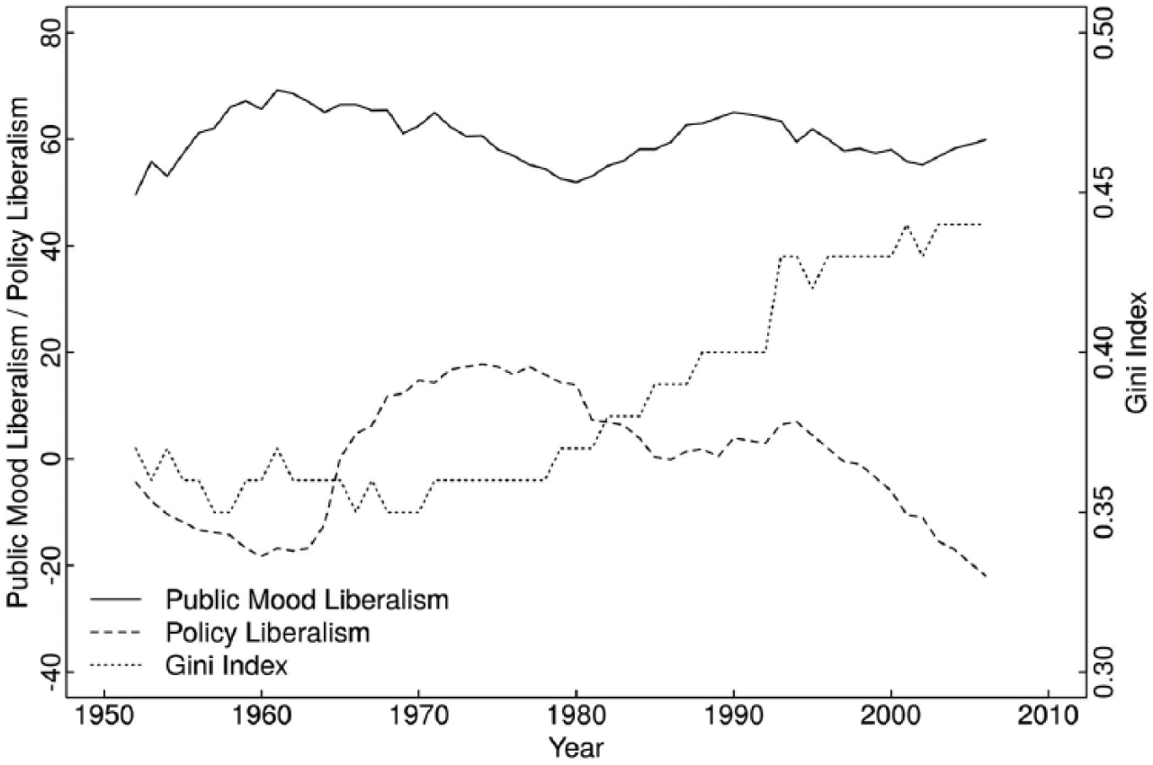
Data from Kelly and Enns’s (2010) table 1 model 2 - relationships are not apparent.

Also, compare Kelly and Enns’s (2010) models 1 and 2 in their table 1 which show the same error correction rate ( ${\hat{α}}_{1}^{*} = - 0.25$ , standard error =0.07). The $t$ -statistics of the six covariates in model 1 are 1.48, -1.85, -0.01, 0.14, -0.64, and -0.46. Why is ${\hat{α}}_{1}^{*}$ exactly the same in the two models – one of which has no $X$ s that matter? Because the models have the same $Y$ and when they interpret ${\hat{α}}_{1}^{*}$ Enns et al. (2016) are confusing $Y$ ’s mean reverting behavior with error correction between $Y$ and $X$ .²¹ Falsely inferring error correction is an easy mistake to make and shows the risks of relying on inferences drawn from ${\hat{α}}_{1}^{*}$ . Researchers are on safer ground when they concentrate on inferences drawn from the $β$ s and long-run multipliers.

Another look at Casillas et al. (2011)

Next, we look at Enns et al.’s defense of Casillas et al. (2011). Casillas et al. use three DVs: Salient Reviews, Non-Salient Reviews, and All Reviews decided in a liberal direction at the US Supreme Court. Enns et al. say:

“We agree with Grant and Lebo that Casillas, Enns, and Wohlfarth were wrong to interpret the $t$ -statistic on the lagged value of salient reversals as evidence of cointegration. This series is stationary, […] so cointegration and long-run relationships should not have been considered.” (Enns et al., 2016: note 24)

What Enns et al. miss, however, is that the differences between Salient Reviews on the one hand and All Reviews and Non-Salient Reviews on the other are ones of degree, not category. These variables are computed anew each year based on the Court’s decisions, making them very unlikely to contain unit roots. However, with T = 45, ADF tests have extremely low power in confirming that.

Enns et al. stand by Casillas et al.’s estimates for All Reviews $({\hat{α}}_{1}^{*} = - 0.83)$ and Non-Salient Reviews $({\hat{α}}_{1}^{*} = - 0.77) .$ Describing their table 1, Casillas et al. say:

“The significant long-run impact of mood on the Court suggests that public opinion also has an effect that is distributed over future time periods. The error correction rate of 0.83 indicates the speed at which this long-term effect takes place. We expect that 83% of the long-run impact of public mood will influence the Court at term $t + 1$ (0.72), an additional 83% of the remaining effect will transpire at term $t + 2$ (0.12), and so on until the total long-run effect has been distributed. Therefore, the Courts long-term responsiveness to public mood occurs rather quickly, as 97% of the total long-run effect of public opinion at term $t$ will be manifested in the justices behavior after just two terms.” (Casillas et al., 2011: 80)

This seemingly incontrovertible conclusion ( $t$ = −5.33) flies in the face of the well-established attitudinal model (Segal and Spaeth, 2002) but is based on short data and a parameter that is difficult to understand. Figure 5 plots out All Reviews and Public Mood. The series look more related than Kelly and Enns’s (2010) data and there may indeed be a close relationship there. However, Casillas et al.’s claim that the error correction rate is 83% implies a much faster rate than what is presented in the T-bill example above.²² Comparing the figures should make it clear that Casillas et al. and Enns et al. are exaggerating error correction – their $α_{1}^{*}$ estimates may be capturing mean reversion or, perhaps, both mean reversion and the long run effects of X.

Figure 5.

Casillas et al.’s (2011) data for their table 1, error correction rate claimed to be 83%.

It is impossible to know the extent to which a negative coefficient on $Y_{t - 1}$ simply indicates that if the level of the series was high (or low) in the last period ∆ $Y$ will be negative (or positive) in the present period due to mean reversion. A significant ${\hat{α}}_{1}^{*}$ can imply different things but it is extremely difficult to distinguish among them. Without complete confidence that the DV has a unit root, judging the extent of error correction in ${\hat{α}}_{1}^{*}$ is unknowable with current GECM techniques. Even MacKinnon CVs are not extreme enough to prevent Type I errors.

To demonstrate, Figure 6 begins with data from Grant and Lebo’s (2016) simulations of fractionally integrated data and shows decreasing values of $d$ associated with increased values and $t$ -statistics for ${\hat{α}}_{1}^{*}$ . Of the many dots, only those on the extreme right of each panel contain I(1) DVs but, as shown in Figure 1(b), many others would provide I(1) evidence.

Figure 6.

Casillas et al.’s (2011) error correction model (ECM) estimates are where they would be if no error correction was occurring.

Figure 6 also includes ${\hat{α}}_{1}^{*}$ estimates from bivariate GECM models for Casillas et al.’s DVs and Public Mood. Enns et al. classify Salient Reviews as stationary and admit the unit root rules should not be applied. But, with ADF results that Non-Salient Reviews and All Reviews are unit roots, they apply the unit root rules and find long-run relationships. However, the low ${\hat{α}}_{1}^{*}$ value and $t$ -statistics are due – at least to some extent – to $Y$ ’s stationary tendencies. Grant and Lebo estimate $d = 0.62$ for both – over 3 standard errors below one.²³ Overlaying the Casillas et al. results by the $d$ estimates shows the findings fall exactly where they would be if no relationship exists between $X$ and $Y$ .

In all, Enns et al.’s (2016: 2) statement: “…we reconsider two of the articles that Grant and Lebo critiqued (CEW, K&E [Casillas et al. and Kelly and Enns]) and we demonstrate that a correct understanding of the GECM indicates that the methods and findings of these two articles are sound,” could only be true if the weakest relationship among our Figures 2, 3, 4, and 5 is Figure 2’s textbook example of cointegration. Enns et al’s blanket statement also misdirects from the fact that they only defend those papers’ least outrageous findings.

In fact, Casillas et al. (2011) misinterpret ${\hat{α}}_{1}^{*}$ and have no real evidence that “the public mood directly constrains the justices’ behavior and the Court’s policy outcomes, even after controlling for the social forces that influence the public and the Supreme Court.” The long run equilibrium the Supreme Court series is reverting to may just be its own mean, not the public’s mood. Finally, even if the independent variables are determining ${\hat{α}}_{1}^{*}$ , Casillas et al.’s approach does not allow them to isolate which $x$ is constraining the Court – the Court’s ideology is an equally likely explanation.

In practice, if you are using the unit root rules in the GECM, you can only easily interpret ${\hat{α}}_{1}^{*}$ if you are certain the DV has a unit root. This is a near impossible task unless one is simulating the data, the time series is quite long, or one has a deep understanding of the data generating process. Given near certain uncertainty, it is best to either find a different model or to rely on other inferences the model provides.

Further thoughts on simulations and replications

Enns et al. (2016: 2) say: “Although our conclusions differ greatly from Grant and Lebo’s recommendations, we do not expect our findings to be controversial. Most of our evidence comes directly from Grant and Lebo’s own simulations.” This statement deserves more attention than there is space for here but the essential point is that Enns et al.’s widespread promotion of MacKinnon CVs is an easy way to reduce Type I error rates in simulations or in practice but these are not the right CVs except when data truly have a unit root. When $d$ or $ρ$ is very close to one, MacKinnon CVs may be close but they are not correct. When $d$ or $ρ$ are further from 1 tests often mistakenly find unit roots.

The properties of the series Enns et al use – in Kelly and Enns, Casillas et al., and elsewhere – do not match the properties of the data they simulate. The consequences of being wrong are to get nonsense results, for example, insisting that 97% of the disequilibrium between Supreme Court decisions and public mood is corrected in two years.

Also, Enns et al. cast doubt when they say Grant and Lebo misused the GECM by replacing the independent variables of published work with shark attacks, tornado fatalities, other nonsense series, and simulated data. Enns et al. are correct that in Grant and Lebo’s replications they did not follow their own advice to set aside regression results where there is no evidence of cointegration. But, of course, that was precisely the point: Grant and Lebo are demonstrating the mistakes made when GECM results are misinterpreted as was done by Kelly and Enns, Casillas et al., and the many published GECM studies.

That is, Grant and Lebo show that if one mimics the methods and interpretation of papers like Casillas et al. (2011) the independent variables do not really matter in terms of getting significant results on the error correction parameter.²⁴ Enns et al. are correct, for instance, that Grant and Lebo’s table 10 replication of Casillas et al. would not show shark attacks and beef consumption to be related to Supreme Court decisions if Grant and Lebo had improved upon Casillas et al.’s methods. Nevertheless, it is notable that with both Kelly and Enns’s (2010) and Ura and Ellis’s (2012) data, some relationships – Grant and Lebo’s table 13 (Republican Mood) and Grant and Lebo’s table E.13 model 3, respectively – between the DVs and variables such as Onion Acreage are strong enough to surpass MacKinnon CVs and conclude cointegration exists. Since the data are unlikely to have unit roots, MacKinnon CVs still are not enough to prevent spurious findings of error correction.

Conclusion

We show that using the unit root rules with series that simply pass the DF test is not enough to avoid overstating findings of error correction. Especially with short time series it is too easy to fail to reject the DF null of non-stationarity and then misunderstand the error correction coefficient. This is a principal reason why the applied literature is replete with incorrect GECM findings and why Grant and Lebo recommend against using the model except in ideal circumstances.

Enns et al.’s “Don’t Jettison the GECM” tries to clarify how to correctly interpret the ECM coefficient but inadvertently shows that while the GECM is viewed as flexible and easy to use it is, in fact, inflexible and extremely easy to misuse. Enns et al. agree that the GECM can work when data are unit roots, cointegrated, and special critical values are used but fail to realize they cannot simply extend those rules to non-unit root data and obtain reliable conclusions.

Indeed, Enns et al. advocate applying the unit root rules to data they know to not have unit roots – autoregressive and fractionally integrated – as well as other series that merely show evidence of a unit root. Moreover, they make their decisions based on the much maligned DF test. Although they say (Enns et al., 2016: 2): “Most of our evidence comes directly from Grant and Lebo’s own simulations” Enns et al. do so while roughly doubling the CVs without proving the practice is correct. Many spurious findings are eliminated this way but MacKinnon CVs and the unit root rules are not enough to overcome the interpretation problems on $α_{1}^{*}$ when data are not I(1).

Grant and Lebo (2016: 27) say: “Error correction between variables is a very close relationship that should be obvious in a simple glance at the data.” The graphs of data we provide here should make it clear that Enns et al.’s claims to have found long run equilibria between political time series in Kelly and Enns (2010) and Casillas et al. (2011) come from the misuse of the method, not the data. Finding long run equilibria across decades of data makes for a story that is interesting but that hinges on a parameter that is often inscrutable. If researchers insist on employing the GECM with data that may not be unit roots they need to focus on the model’s other parameters.

Footnotes

Declaration of Conflicting Interest

The authors declare that there is no conflict of interest.

Funding

This research received no specific grant from any funding agency in the public, commercial, or not-for-profit sectors.

Notes

Carnegie Corporation of New York Grant

This publication was made possible (in part) by a grant from Carnegie Corporation of New York. The statements made and views expressed are solely the responsibility of the author.

References

Bannerjee

Dolado

Galbraith

. (1993) Integration, Error Correction, and the Econometric Analysis of Non-Stationary Data. Oxford, UK: Oxford University Press.

Box-Steffensmeier

Smith

(1996) The dynamics of aggregate partisanship. American Political Science Review 90(3): 567–580.

Box-Steffensmeier

DeBoef

Lin

T-M

(2004) The dynamics of the partisan gender gap. American Political Science Review 98(3): 515–528.

Byers

Davidson

Peel

(2000) The dynamics of aggregate political popularity: Evidence from eight countries. Electoral Studies 19(1): 49–62.

Casillas

Enns

Wohlfarth

(2011) How public opinion constrains the US Supreme Court. American Journal of Political Science 55(1): 74–88.

Clarke

Lebo

(2003) Fractional (co)integration and governing party support in Britain. British Journal of Political Science 33(2): 283–301.

DeBoef

Granato

(1997) Near-integrated data and the analysis of political relationship. American Journal of Political Science 41(2): 619–640.

DeBoef

Granato

(1999) Testing for cointegrating relationships with near-integrated data. Political Analysis 8(1): 99–117.

DeBoef

Keele

(2008) Taking time seriously. American Journal of Political Science 52(1): 184–200.

10.

Dickey

Fuller

(1979) Distribution of the estimators for autoregressive time series with a unit root. Journal of the American Statistical Association 74(336): 427–431.

11.

Engle

Granger

CWJ

(1987) Co-integration and error correction: Representation, estimation, and testing. Econometrica 55(2): 251–276.

12.

Enns

Kelly

Masaki

. (2016) Don’t jettison the general error correction model just yet: A practical guide to avoiding spurious regression with the GECM. Research & Politics 3(2): DOI: 2053168016643345

13.

Ericsson

MacKinnon

(2002) Distributions of error correction tests for cointegration. The Econometrics Journal 5(2): 285–318.

14.

Esarey

(2016) Fractionally integrated data and the autodistributed lag model: Results from a simulation study. Political Analysis 24(1): 42–49.

15.

Gil-Alana

(2003) Testing of fractional cointegration in macroeconomic time series. Oxford Bulletin of Economics and Statistics 65(4): 517–529.

16.

Grant

(2015) Fractional integration in short samples: Parametric versus semiparametric methods. Available at: https://www.researchgate.net/publication/277586072_Fractional_Integration_in_Short_Samples_Parametric_versus_Semiparametric_Methods (accessed 1 June 2017).

17.

Grant

Lebo

(2016) Error correction methods with political time series. Political Analysis 24(1): 3–30.

18.

Helgason

(2016) Fractional integration methods and short time series: Evidence from a simulation study. Political Analysis 24(1): 59–68.

19.

Keele

Linn

Webb

(2016) Treating time with all due seriousness. Political Analysis 24(1): 31–41.

20.

Kelly

Enns

(2010) Inequality and the dynamics of public opinion: The self-reinforcing link between economic inequality and mass preferences. American Journal of Political Science 54(4): 855–870.

21.

Lebo

(2008) Divided government, united approval: The dynamics of Congressional and Presidential approval. Congress and the Presidency 35(2): 1–16.

22.

Lebo

Cassino

(2007) The aggregated consequences of motivated reasoning and the dynamics of partisan presidential approval. Political Psychology 28(6): 719–746.

23.

Lebo

Grant

(2016) Equation balance and dynamic political modeling. Political Analysis 24(1): 69–82.

24.

Lebo

Weber

(2015) An effective approach to the repeated cross-sectional design. American Journal of Political Science 59(1): 242–258.

25.

Lebo

Young

(2009) The comparative dynamics of party support in Great Britain: Conservatives, Labour and the Liberal Democrats. Journal of Elections, Public Opinion and Parties 19(1): 73–103.

26.

Lebo

McGlynn

Koger

(2007) Strategic party government: Party influence in Congress, 1789–2000. American Journal of Political Science 51(3): 464–481.

27.

Lebo

Walker

Clarke

(2000) You must remember this: Dealing with long memory in political analyses. Electoral Studies 19(1): 31–48.

28.

Murray

(1994) A drunk and her dog: an illustration of cointegration and error correction. The American Statistician 48(1): 37–39.

29.

Segal

Spaeth

(2002) The Supreme Court and the Attitudinal Model Revisited. New York, NY: Cambridge University Press.

30.

Stock

Watson

(2011) Introduction to Econometrics. 3rd edition. Boston, MA: Addison-Wesley.

31.

Ura

Ellis

(2012) Partisan moods: Polarization and the dynamics of mass party preferences. The Journal of Politics 74(1): 277–291.

32.

Volscho

Kelly

(2012) The rise of the super-rich power resources, taxes, financial markets, and the dynamics of the top 1 percent, 1949 to 2008. American Sociological Review 77(5): 679–699.

The general error correction model in practice

Abstract

Keywords

Introduction

Points of agreement

The GECM can work when all the series contain unit roots and are jointly cointegrated

The GECM is possible but not recommended when all series are stationary

Point of likely disagreement

Points of disagreement

The GECM in practice when we are too quick to find unit roots

Another look at Kelly and Enns (2010)

Another look at Casillas et al. (2011)

Further thoughts on simulations and replications

Conclusion

Footnotes

Declaration of Conflicting Interest

Funding

Notes

Carnegie Corporation of New York Grant

References