Sage Journals: Discover world-class research

Abstract

In a recent issue of Political Analysis, Grant and Lebo authored two articles that forcefully argue against the use of the general error correction model (GECM) in nearly all time series applications of political data. We reconsider Grant and Lebo’s simulation results based on five common time series data scenarios. We show that Grant and Lebo’s simulations (as well as our own additional simulations) suggest the GECM performs quite well across these five data scenarios common in political science. The evidence shows that the problems Grant and Lebo highlight are almost exclusively the result of either incorrect applications of the GECM or the incorrect interpretation of results. Based on the prevailing evidence, we contend the GECM will often be a suitable model choice if implemented properly, and we offer practical advice on its use in applied settings.

Keywords

time series ecm error correction model spurious regression methodology Monte Carlo simulations

In a recent issue of Political Analysis, Taylor Grant and Matthew Lebo author the lead and concluding articles of a symposium on time series analysis. These two articles argue forcefully against the use of the general error correction model (GECM). In their lead article, Grant and Lebo declare: “we recommend the GECM in only one rare situation: when all of the variables are strictly unit-root series, $Y_{t}$ is unbounded, $Y_{t}$ and $X_{t}$ are cointegrated, and the MacKinnon critical values are used… A careful look at the applied literature in political science will not find any examples that meet all those criteria” (p.27). They reiterate this point in their concluding article, stating: “we remain skeptical that the GECM is a reliable model except in the very rare case where one has unbounded unit-root variables that are cointegrated with each other” (p.80). Given the popularity of the GECM for time series analysis (e.g. Beck and Katz, 2011; Blaydes and Kayser, 2011; Jennings, 2013; Layman et al., 2010; Soroka et al., 2015), Grant and Lebo’s insistence that the GECM is inappropriate for political science applications would seem to hold major implications for time series practitioners.¹

Grant and Lebo identify two primary concerns with the GECM. First, when time series are stationary, the GECM cannot be used as a test of cointegration. This is a useful and often under-appreciated point.² However, if this were Grant and Lebo’s only concern, their analysis would not fundamentally alter the conclusions of past research and could be easily dealt with in future studies by not using the GECM to test for cointegration with stationary time series. Grant and Lebo’s second concern is much more troubling. They argue that across most (and perhaps all) political science time series, the GECM will produce “an alarming rate of Type I errors” (p.4). This threat of spurious findings is the primary reason Grant and Lebo advocate abandoning the GECM.

If the GECM regularly produces spurious results, scholars would indeed be well-advised to abandon this approach. However, the problems Grant and Lebo highlight follow almost entirely from either incorrect applications of the GECM or incorrect interpretation of results. Indeed, a careful examination of Grant and Lebo’s results, as well as the other contributions to the Political Analysis symposium, shows the GECM performs quite well across a variety of common data scenarios in political science. In this article, we examine five of the scenarios that Grant and Lebo consider and we find that for four of the data scenarios, if applied correctly the GECM can be estimated without concern for spurious relationships. With the fifth data type (fractionally integrated series), the GECM sometimes offers a suitable approach.³ Our analysis pays particularly close attention to the cases of bounded unit roots and near-integrated time series. We devote extra attention to these types of time series because they are common in political science and because none of the other symposium articles reconsider Grant and Lebo’s claims about these types of data.⁴ We show that when applied correctly, there is no inherent problem when using the GECM with bounded unit roots or near-integrated data.

Although our conclusions differ greatly from Grant and Lebo’s recommendations, we do not expect our findings to be controversial. Most of our evidence comes directly from Grant and Lebo’s own simulations. We also support our claims with additional simulation results. Although our findings are straightforward, our conclusions about the GECM are important for multiple reasons. First, a correct understanding of the GECM holds implications for how we understand existing research. Grant and Lebo identified five prominent articles and in each case they critiqued the authors’ use of the GECM. Grant and Lebo also pointed out that none of the other symposium articles provide “a defense of any GECM results published by a political scientist” (p.70). Our findings show that Grant and Lebo were too quick to criticize these researchers’ use of the GECM. Indeed, we reconsider two of the articles that Grant and Lebo critiqued (Casillas et al., 2011; Kelly and Enns, 2010) and we demonstrate that a correct understanding of the GECM indicates that the methods and findings of these two articles are sound.

Understanding the GECM also holds implications for future research. For time series analysis, Grant and Lebo recommend fractional integration (FI) methods. Although FI methods are certainly an important statistical approach (e.g. Box-Steffensmeier et al., 1998; Box-Steffensmeier and Tomlinson, 2000; Clarke and Lebo, 2003), substantial disagreement exists regarding their utility for political science data (Box-Steffensmeier and Helgason, 2016).⁵ Given the debate about the utility of FI methods (especially with short time series), it is important for researchers to know when the GECM avoids the errors that Grant and Lebo ascribe to it. Until alternate methods are shown to perform better, based on our findings we recommend that researchers use the GECM for bounded unit roots (when statistical tests indicate the dependent variable contains a unit root and cointegration is present) and with near-integrated data (again, cointegration must be established when statistical tests suggest a unit root).⁶ We also remind readers that the GECM is appropriate with FI data in some contexts (Esarey, 2016; Helgason, 2016) and it is appropriate with stationary time series (although we point out that the mathematically equivalent autodistributed lag model (ADL) is less likely to produce errors of researcher interpretation with stationary data).

We conclude with a detailed summary of our recommendations for time series practitioners, highlighting where we agree with Grant and Lebo and where our recommendations differ. The conclusion also discusses avenues for future research. These include studying the performance of the GECM with other types of time series. Wlezien (2000), for example, discusses “combined” time series (which contain both integrated and stationary processes) and he shows they can be modeled with a GECM. Future research also needs to continue to evaluate the performance of FI techniques. Of particular interest is resolving the debate between Lebo and Grant (2016) and Keele et al. (2016) regarding how long a time series must be to reliably estimate the FI parameter $d$ and demonstrating whether Grant and Lebo’s proposed fractional error correction model (FECM) is able to identify true relationships in short time series.

Reconsidering five of Grant and Lebo’s data scenarios

In this section, we revisit Grant and Lebo’s first five data scenarios. We find that across all five scenarios, the GECM typically avoids spurious relationships. We explain why our results differ from Grant and Lebo’s conclusions and highlight when we agree with their recommendations.

Case 1: The dependent variable contains a unit root, $I (1)$

Grant and Lebo begin with a very important, and often forgotten, point. They show that if the dependent and independent variables contain a unit root, cointegration must be established prior to interpreting the results of a GECM (see also Enns et al., 2014).⁷ Grant and Lebo explain, “Without cointegration, however, the model is unbalanced and the practitioner should set aside the estimates and choose a different specification” (p.7).⁸ Grant and Lebo also correctly emphasize that when $Y_{t}$ contains a unit root and the GECM is used to test for cointegration, “non-standard critical values must be used (Ericsson and MacKinnon, 2002) to evaluate cointegration” (p.8). Specifically, the $t$ -statistic associated with $α_{1}$ (i.e. the error correction rate) in the GECM

Δ Y_{t} = α_{0} + α_{1} Y_{t - 1} + β_{0} Δ X_{t} + β_{1} X_{t - 1} + ε_{t},

(1)

must be less than the corresponding critical value in Ericsson and MacKinnon (2002). Grant and Lebo’s Table 2 (second row) confirms that when an analyst uses the appropriate critical values, this cointegration test performs well even when $T = 60$ and regardless of the number of predictors specified in the model. Since Grant and Lebo only find (incorrect) evidence of cointegration about 5 per cent of the time, if researchers follow Grant and Lebo’s recommendation to set aside estimates when there is no evidence of cointegration, incorrect evidence of a long-run relationship (i.e. $β_{1}$ in Equation (1)) could never exceed 5 per cent with integrated data (because 95% of potential analyses have been set aside).

At first glance, the bottom row of Grant and Lebo’s Table 2 might appear to contradict this statement, because these results show that Grant and Lebo incorrectly rejected the null hypothesis that $β_{1} = 0$ after testing for cointegration between 14 and 47 per cent of the time. However, these results are based on cointegration tests with incorrect critical values.⁹ Thus, the bottom row of Grant and Lebo’s Table 2 should be read as evidence of the importance of using the correct MacKinnon critical values when testing for cointegration, not evidence of spurious relationships with the GECM. Their Table 2 also shows that although ${\hat{α}}_{1}$ provides accurate tests of cointegration (when researchers use the correct critical values), ${\hat{α}}_{1}$ (which typically ranges between 0 and $- 1.0$ ) is biased downward (i.e. more negative). Typically, this bias will not pose a problem for researchers. First, the bias does not affect the estimates of $β_{0}$ or $β_{1}$ (because these estimated short- and long-run effects do not depend on ${\hat{α}}_{1}$ ). Second, the magnitude of the bias is small.¹⁰ Third, the bias influences the estimate of the total effect of $X_{t}$ on $Y_{t}$ (i.e. the long-run multiplier (LRM)) in a conservative direction. The conservative bias emerges because a smaller (more negative) ${\hat{α}}_{1}$ will decrease the estimated LRM (because the LRM equals $\frac{β_{1}}{α_{1}}$ ), leading researchers to conclude a smaller total effect of $X_{t}$ on $Y_{t}$ . Because ${\hat{α}}_{1}$ indicates how quickly the total effect of $X_{t}$ on $Y_{t}$ occurs through future time periods, researchers must also be aware that if ${\hat{α}}_{1}$ is biased downward, the true rate of error correction likely takes longer than ${\hat{α}}_{1}$ implies. When discussing the LRM or the rate of error correction, researchers must acknowledge how the bias in ${\hat{α}}_{1}$ that Grant and Lebo identified could affect their estimates. However, as long as researchers acknowledge this bias in ${\hat{α}}_{1}$ , we agree with Grant and Lebo that the GECM can be used with integrated data that are cointegrated.

Case 2: The dependent variable is a bounded unit root

Grant and Lebo’s second case considers bounded unit roots, which are time series that “can exhibit the perfect-memory of integrated data” but are bound between an upper and lower limit (p.10). Grant and Lebo cite the public’s policy mood as an example (Stimson, 1991). They find that policy mood contains a unit root, but because it is based on survey percentages, it is clearly bound between 0 and 100. According to Grant and Lebo, bounded unit roots should not be analyzed with a GECM. They write, “Even if we find series that are strictly unit-roots and we use MacKinnon CVs, mistakes are still rampant if our dependent variable is one of the vast majority of political times series that is bounded” (p.12).

A reconsideration of Grant and Lebo’s simulations demonstrates, however, that the GECM performs no worse with bounded unit roots than it does with the integrated time series discussed in Case 1 (where Grant and Lebo recommend the use of the GECM). First, consider Grant and Lebo’s finding that, “Boundedness does not seem to affect the estimation of $β_{1}$ or $β_{0}$ ” (pp.11–12). This is an important result because these parameters correspond with the long-run and immediate relationships between $X_{t}$ and $Y_{t}$ , which are typically what researchers are most interested in testing. Grant and Lebo’s concern is that the GECM yields incorrect inferences about cointegration with bounded unit roots. Consistent with this claim, their Table 3 shows that the GECM incorrectly shows evidence of cointegration between unrelated series more than 5 per cent of the time. However, the inflated rate of Type I errors associated with the cointegration test results because of an incorrect application of the GECM.¹¹

To understand why the results in Grant and Lebo’s Table 3 are problematic, recall that Grant and Lebo’s key point about bounded unit roots is that despite containing a unit root, bounded unit roots behave differently than pure $I (1)$ series. Specifically, “as the series nears its upper and lower thresholds it tends towards mean reversion” (Grant and Lebo, Supplementary Materials, p.13). This mean reversion at set bounds can produce a constant mean with a constant variance, which means the series would behave as if stationary. If the series behaves as if it is stationary, even if the data generating process (DGP) contains a unit root, these sample properties must inform the statistical analysis. As Grant and Lebo write, “Analysts should deal with the properties of the data sample they have and not make arguments about asymptotics” (p.72).¹² Thus, even if we know the DGP to contain a unit root, if the bounded nature of the data produces a series that mimics a stationary time series, we must take this into account.

As noted above (also see Case 3 below), Grant and Lebo show that tests of cointegration based on a GECM will incorrectly find evidence of cointegration too often if the dependent variable is stationary. This realization provides a rather simple modeling strategy for bounded unit roots. When a bounded unit root behaves as if it is stationary, the GECM should not be used to test for cointegration. When a bounded unit root behaves as if it contains a unit root, the GECM should be appropriate. To test whether this strategy avoids Type I errors, we replicate Grant and Lebo’s bounded unit root simulations, adding a test for the time series properties of $Y_{t}$ . Specifically, we use Grant and Lebo’s simulation code to generate dependent series to be bounded unit roots. These series depend on three parameters: the range of the bounds, which is set to 1–100 and 49–71, the variance of the disturbance term, which is set to 1, 2, or 3, and the series length, where $T$ equals 60, 100, or 150.¹³ Following Grant and Lebo, the predictors are integrated time series $I (1)$ .

After generating these series, we use an augmented Dickey Fuller (ADF) test to evaluate whether we reject the null hypothesis of a unit root in the dependent series. At first, our use of an ADF test may seem surprising. It is well known that ADF tests are underpowered against the alternative hypothesis of stationarity (Blough, 1992; Cochrane, 1992). Thus, the ADF may incorrectly conclude that a series that behaves as if stationary follows a unit root process in the observed data. However, this means we are biasing our simulations against support for the GECM since we are more likely to incorrectly conclude the series contains a unit root and thus inappropriately utilize the GECM as a test of cointegration (thereby inflating the rate of Type I errors with those cointegration tests). If the ADF rejects the null of a unit root, we do not use the GECM to test for cointegration. Even though the true DGP in our simulations is a bounded unit root, if the series behave as if stationary (because the bounds and mean reversion generate a series with a constant variance and mean), the GECM should not be used to test for cointegration. Not only would the cointegration test be wrong if the dependent series behaves as if stationary, but we have no reason to expect a cointegrating relationship between an integrated predictor and an outcome variable that appears stationary (Keele et al., 2016).

Table 1 reproduces Grant and Lebo’s original results (from their Table 3, p.11) and the results from our simulations. Recall that our simulations are identical to Grant and Lebo’s except we do not use the GECM to test for cointegration if an ADF test on $Y_{t}$ rejects the null of a unit root. We add this step because a stationary time series cannot be cointegrated with an integrated time series (Keele et al., 2016), rendering it unnecessary to test for cointegration, and because tests for cointegration with a stationary time series will produce biased results (Grant and Lebo, 2016). First, note that Grant and Lebo’s results show that naively estimating a GECM will produce incorrect evidence of cointegration more than 5 per cent of the time, and these errors will increase as $T$ increases, the variance increases, and with the more limited bounds of 49 to 71. These results are not surprising because as discussed above, each of these conditions (i.e. longer $T$ , greater variance, and narrower bounds) would increase the mean reversion of the series.

Table 1.

The percentage of simulations that provide incorrect evidence of cointegration based on Grant and Lebo’s Table 3 and based on first testing for a unit root.

	Bivariate
DV bounds:	(1–100)	(49–71)	(1–100)	(49–71)	(1–100)	(49–71)
Model type:	$T = 60$ , $σ = 1$		T=60, σ=2		T=60, $σ = 3$
Grant & Lebo reproduction	6.0	7.7	6.1	9.9	6.1	12.4
With unit root test	2.5	3.6	2.8	4.1	3.0	5.0
	T=100, $σ = 1$		T=100, $σ = 2$		T=100, $σ = 3$

Grant & Lebo reproduction	7.0	10.5	7.6	14.8	8.1	23.1
With unit root test	2.7	3.6	3.2	4.7	3.4	6.2

	$T = 150$ , σ=1		$T = 150$ , $σ = 2$		T=150, $σ = 3$
Grant & Lebo reproduction	6.5	12.2	7.6	20.5	8.4	45.6
With unit root test	3.0	4.0	3.3	5.8	3.3	5.9
	Multivariate (2 IVs)
DV bounds:	(1–100)	(49–71)	(1–100)	(49–71)	(1–100)	(49–71)
Model type:	$T = 60$ , $σ = 1$		T=60, σ = 2		T=60, σ = 3
Grant & Lebo reproduction	6.2	7.8	6.4	10.6	6.6	12.6
With unit root test	3.6	4.8	4.0	5.1	4.3	5.9

	T=100, σ = 1		T=100, $σ = 2$		$T = 100$ , σ = 1
Grant & Lebo reproduction	6.2	9.6	6.6	13.9	7.0	20.8
With unit root test	3.4	4.4	4.0	5.6	4.4	7.4

	$T = 150$ , $σ = 1$		T=150, σ = 2		T=150, σ = 3
Grant & Lebo reproduction	6.8	11.5	7.7	18.5	8.4	38.5
With unit root test	3.6	5.3	4.3	7.6	4.4	6.3

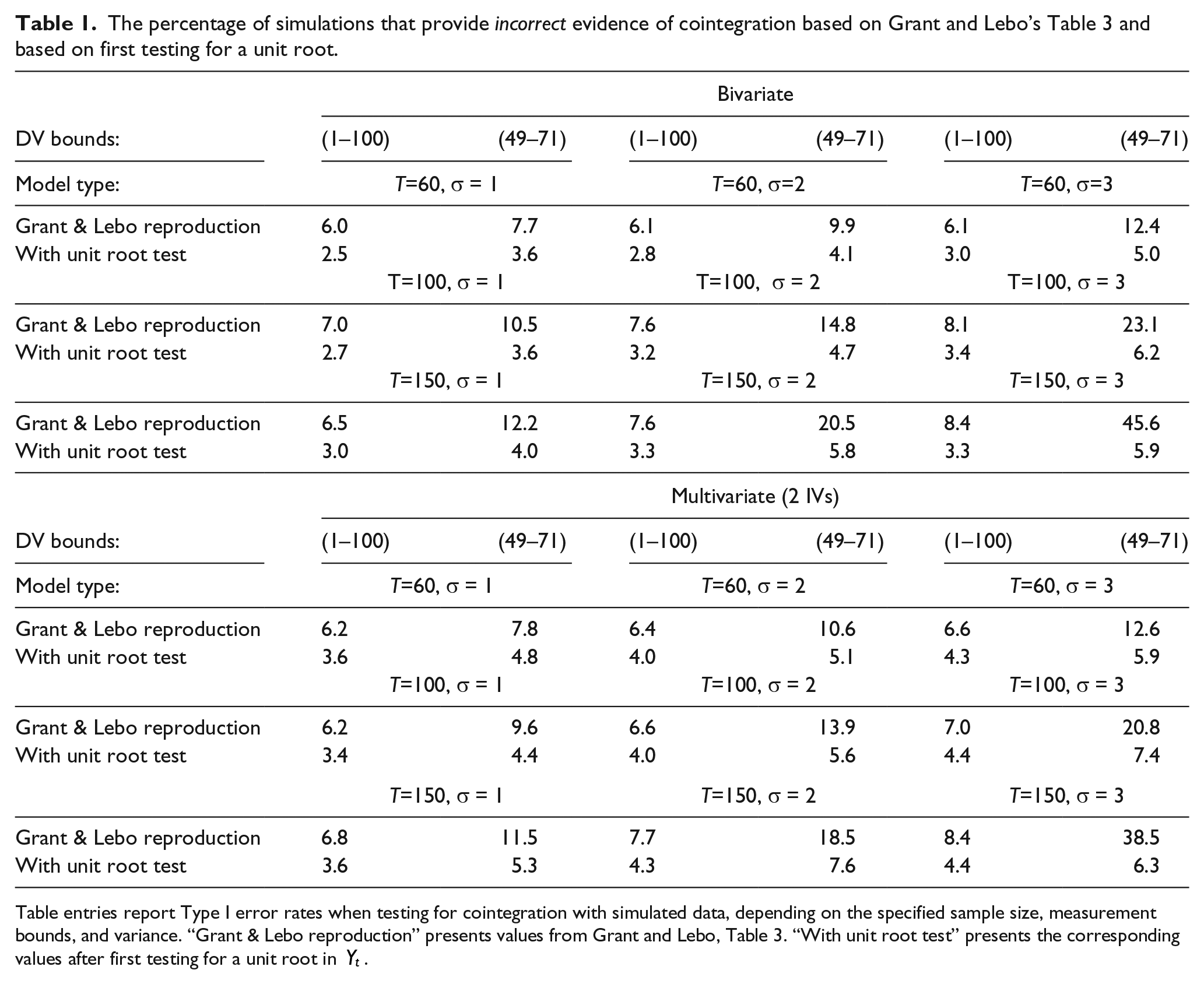
Table entries report Type I error rates when testing for cointegration with simulated data, depending on the specified sample size, measurement bounds, and variance. “Grant & Lebo reproduction” presents values from Grant and Lebo, Table 3. “With unit root test” presents the corresponding values after first testing for a unit root in $Y_{t}$ .

Our primary interest is evaluating whether the GECM yields correct inferences if we first test the sample properties of the bounded unit root. To test this expectation, the “With Unit Root Test” rows only use the GECM to test for cointegration if the ADF test does not reject the null hypothesis of a unit root in the dependent series. Across all parameters, the Type I error rate is about 5 per cent. By first diagnosing the time series properties of the dependent series (which is standard practice in time series analysis), we avoid the Type I errors in the cointegration tests. These results show that there is no inherent problem with using the GECM with bounded unit roots.¹⁴ This is an important result. Grant and Lebo state, “Even if we find series that are strictly unit-roots and we use MacKinnon CVs, mistakes are still rampant if our dependent variable is one of the vast majority of political times series that is bounded” (p.12). Yet, the results in Table 1 show that if we follow these guidelines (i.e. find evidence of unit–roots and use MacKinnon critical values), the mistakes Grant and Lebo found essentially disappear.

In addition to offering guidance about the appropriate use of the GECM, these simulation results hold implications for Grant and Lebo’s analysis of Kelly and Enns (2010). Grant and Lebo use Kelly and Enns’ analysis of the relationship between income inequality and policy mood to illustrate the pitfalls of analyzing a bounded unit root with a GECM. Specifically, based on Kelly and Enns’ analysis, Grant and Lebo conclude that there is “No cointegration” and thus the “GECM model [is] inappropriate” (p.26). Yet, looking at Kelly and Enns’ most parsimonious analysis (Table 1, Column 2) we find clear evidence of cointegration.¹⁵ We select the most parsimonious specification because in Keele, Linn, and Webb’s first contribution to the symposium, they suggested that Kelly and Enns over-fit their model. By focusing on this parsimonious model (which Keele, Linn, and Webb did not consider) we mitigate concerns that the results are due to over-fitting the model. The evidence of cointegration in Kelly and Enns’ analysis combined with the simulation results above in Table 1 support the use of the GECM. Grant and Lebo also conclude that there is “No support for short- or long-term effect of income inequality on public mood” (p.26). This conclusion is surprising because, as noted above, Grant and Lebo conclude that “Boundedness does not seem to affect estimation of $β_{1}$ or $β_{0}$ ” (pp.11–12) and $β_{0}$ and $β_{1}$ reflect Kelly and Enns’ estimates of the short- and long-term relationships between income inequality and public mood (see Grant and Lebo’s Equation (5)). Grant and Lebo’s conclusion that the estimates of $β_{0}$ and $β_{1}$ are not affected by boundedness further validates Kelly and Enns’ estimates of these parameters.

Since the various simulations validate Kelly and Enns’ estimates and conclusions about cointegration, we wondered why Grant and Lebo’s replication of Kelly and Enns with nonsense regressions produced spurious results. In their nonsense regressions, Grant and Lebo replicated Kelly and Enns’ analysis substituting the key predictor variables for variables that are surely unrelated to the public’s policy mood: beef consumption, coal emissions, tornado fatalities, and onion acreage (see Grant and Lebo’s Table E.13). Grant and Lebo write, “Based on our past replications and simulations we expect spurious regressions, and that is what we find” (Grant and Lebo, supplementary materials, p.43). This conclusion depends, however, on an incorrect application of the GECM. Across the eight nonsense regressions, none show evidence of cointegration.¹⁶ If Grant and Lebo followed their own advice to “set aside the estimates” without cointegration, they would never have reported these results from these nonsense regressions.¹⁷ The spurious results in their nonsense regressions result because they did not test for cointegration. We should also note that even if the GECM was implemented correctly, we do not recommend the use of atheoretical variables to demonstrate the possibility of spurious findings. Instead, we recommend the standard approach of simulating data and conducting Monte Carlo experiments.¹⁸

Grant and Lebo’s final critique of Kelly and Enns comes from their Tables E.16 and E.17, where they re–analyze Kelly and Enns’ data with a FECM and find no significant relationships in the data. What Grant and Lebo fail to consider is the possibility that FECMs under-identify true relationships in small samples. Since Grant and Lebo’s fractional differencing analyses failed to fully replicate four out of five influential articles, this is a critical consideration. In all of their simulations, Grant and Lebo never report how often fractional differencing methods identify true relationships. Helgason (2016) considered prediction error and found that the performance of the FECM depends heavily on whether short-term dynamics are present and the sample size, but he did not test how often FECMs correctly identify true relationships. We also do not know how the FECM performs if applied to data that are not fractionally integrated. If the FECM is overly conservative, Grant and Lebo’s re-analysis and critiques of the other articles would also be highly problematic. This is an important area for future research.

Case 3: The dependent variable and all independent variables are stationary

As we noted earlier, Grant and Lebo make an important contribution by highlighting the fact that $α_{1}$ in a GECM cannot be used as a test of cointegration when the dependent variable is stationary. Grant and Lebo also claim that the GECM is inappropriate with a stationary dependent variable. In their concluding article, they emphasize, “the increased risk of Type I errors for $X$ when using the GECM rather than the ADL” (p.70). In their response to Grant and Lebo, Keele, Linn, and Webb challenge this conclusion by stating the equivalence of the ADL and GECM is “mathematical fact” (p.32).¹⁹ Indeed, from a mathematical standpoint, since the ADL is appropriate with a stationary dependent variable, the GECM must also be appropriate in this scenario.

Here we wish to clarify that the increased risk of Type I errors that Grant and Lebo refer to is due entirely to the potential for incorrect interpretation of GECM results. Although the GECM and ADL contain the exact same information, the two models present this information differently. When researchers fail to realize that the two models present information differently, errors of interpretation can emerge. Thus, we agree with Grant and Lebo that when the dependent variable is stationary, the parameterization of the GECM is more likely than the ADL to lead to errors of interpretation. Specifically, when estimating a GECM with a stationary $Y_{t}$ , researchers must remember not to interpret $α_{1}$ as a test of cointegration and researchers cannot directly consider the estimate for $β_{1}$ . Instead, to obtain the estimated lagged effect of $X_{t - 1}$ on $Y_{t}$ , $β_{0}$ must be subtracted from $β_{1}$ (and the corresponding standard error must be calculated). Estimating an ADL avoids these considerations. Although the true Type I error rate for ADLs and GECMs is identical, we agree with Grant and Lebo that with a stationary dependent variable the ADL is less likely to lead to errors of interpretation.

Case 4: The dependent variable is strongly autoregressive/near-integrated

Grant and Lebo’s fourth case focuses on near-integrated data, which are time series with a root close to, but not quite, unity (Phillips, 1988). Grant and Lebo again draw a confusing distinction between the ADL and GECM. In their first article, they write: “Our findings for the ADL match those of De Boef and Granato (1997), who find that the model has acceptable spurious regression rates with near–integrated data. But we also find that this does not translate for the same data in the GECM” (p.15). They present additional simulation results in support of this claim in their concluding article, stating that when estimating a GECM, “With sixty observations there is a significant threat of Type I errors” (p.75). Because the ADL and GECM are the same model, as with the stationary dependent variable example above, the threat of errors stems entirely from potential researcher errors. Because the ADL and GECM are mathematically equivalent, and since Grant and Lebo found evidence that the ADL avoids spurious correlations (see their Table 6), the same must be true for the GECM. There is no inherent problem with the GECM and near-integrated data. If the GECM is implemented correctly, no problems emerge.

Here we review Grant and Lebo’s simulation results to illustrate potential errors that researchers need to avoid. One potential error is evaluating $β_{1}$ in the GECM without first testing for cointegration. This inflated Type I error rate is evident in Table 1 of Grant and Lebo’s concluding article, where they report false rejection rates as high as 24 per cent for the null hypothesis that the long run multiplier (i.e. $\frac{β_{1}}{α_{1}}$ ) equals zero for all simulations. Because the long-run multiplier assumes a cointegrating relationship between $X_{t}$ and $Y_{t}$ , researchers should not evaluate whether the LRM is significant unless first finding evidence of cointegration. As Grant and Lebo’s lead article explained, estimates should be “set aside” if there is no evidence of cointegration. It is the failure to first test for cointegration, not the GECM, that leads to the inflated false rejection rate in Table 1 of Grant and Lebo’s concluding article.²⁰

A second error can result from using the incorrect critical values when testing for cointegration with $α_{1}$ . For example, the “GECM Model” results that Grant and Lebo report in Table 6 (of their lead article) are based on a test of cointegration that uses standard (one–tailed) critical values instead of the appropriate MacKinnon critical values. To illustrate the consequences of this error, we consider the results in Grant and Lebo’s Tables G.1 through G.5 (in their supplementary materials). Although the results Grant and Lebo reported in the text of their article did not use the appropriate critical values, Tables G.1 through G.5 in their supplementary materials did include results based on the correct MacKinnon critical values. Thus, we can rely on these tables from their supplementary materials to evaluate the performance of the GECM when analyzed correctly. In Table 2 we reproduce a summary of the results from Grant and Lebo’s Tables G.1–G.5. To clarify their findings, we make two changes to how they reported their results. First, instead of reporting the number of false rejections, we report the per cent of false rejections. Second, we account for the fact that each additional parameter estimated increases the likelihood of falsely rejecting the true null hypothesis. This step is necessary because Grant and Lebo report how many times one or more significant relationships emerge. Since $k$ predictors increases the likelihood of finding a significant relationship $k$ times, we divide the number of false rejections reported by Grant and Lebo by $k$ . Again, although we make these changes for ease of interpretation, all values in our Table 2 are based directly on Grant and Lebo’s Tables G.1–G.5.

Table 2.

The percentage of spurious relationships for near-integrated series, results from Grant and Lebo Tables G.1–G.5 ( $T = 60$ ).

ρ_y	ρ_x	$β_{0} Δ X_{t}$					$β_{1} X_{t - 1}$
		Number of predictors					Number of predictors
		1	2	3	4	5	1	2	3	4	5
0.90	$I (1)$	5.92	6.07	5.69	5.75	5.69	5.19	3.66	2.67	2.17	1.72
0.95	$I (1)$	6.05	6.14	5.71	5.77	5.71	3.95	2.76	2.05	1.60	1.28
0.99	$I (1)$	6.07	6.06	5.87	5.75	5.80	3.30	2.26	1.69	1.26	1.04
0.90	0.90	5.85	5.97	5.79	5.75	5.64	3.63	2.63	1.96	1.45	1.13
0.95	0.95	6.19	6.07	6.07	5.84	5.77	3.13	2.18	1.66	1.28	1.06
0.99	0.99	6.11	6.21	5.92	5.80	5.78	3.07	2.06	1.54	1.16	1.00
0.90	$I (0)$	5.61	5.46	5.04	5.02	4.96	0.89	0.39	0.24	0.11	0.04
0.95	$I (0)$	5.61	5.53	5.00	4.98	4.96	0.52	0.20	0.11	0.05	0.03
0.99	$I (0)$	5.51	5.55	4.98	5.04	4.90	0.36	0.10	0.06	0.03	0.02

Notes: Long-term estimates ( $β_{1}$ ) reflect the percentage of spurious relationships when the MacKinnon critical values provide evidence of cointegration. Because Grant and Lebo report the number of simulations with at least one significant predictor variable, we divide this number by the number of predictors in the model to account for the fact that k additional predictors increase the number of parameter estimates that could be significant k times.

The left half of our Table 2 reports the false rejection rates for $β_{0}$ , which represents the immediate effect of $X_{t}$ on $Y_{t}$ . Across all scenarios, the false rejection rate is close to the expected 5 per cent. This is an important result. Even without testing for cointegration, the immediate relationship is estimated correctly. Of course, this must be the case. In the GECM $β_{0}$ corresponds with the coefficient on $X_{t}$ in the ADL, which is what Grant and Lebo report in the top half of their Table 6. Since they did not observe evidence of spurious regression with their ADL estimates, we do not expect to observe spurious results for the identical estimates based on the GECM.

As noted above, the bottom half of Grant and Lebo’s Table 6 found false rejection rates above 5 per cent because they did not use the appropriate MacKinnon critical values. The right half of Table 2 reports the same information (i.e. the false rejection rate for $α_{1} = 0$ and $β_{1} = 0$ ) when the correct critical values are used. These results are based entirely on Grant and Lebo’s Tables G.1–G.5. When we use the correct critical values (as Grant and Lebo did in their Tables G.1–G.5), the percentage of false rejections is always below 5 per cent.²¹

Grant and Lebo’s lead and concluding articles recommend that the GECM should not be estimated with near-integrated data and short time series. We agree that if scholars implement the GECM incorrectly with near-integrated data, incorrect results will emerge. However, Grant and Lebo’s simulation results (based on the ADL as well as the GECM) show that if the GECM is implemented and interpreted correctly (i.e. long-run relationships in the GECM are only considered if there is evidence of cointegration), it is completely appropriate with near-integrated data.

Case 5: The dependent variable is fractionally integrated, (0, d, 0) and $0 < d < 1$

Grant and Lebo’s fifth case focuses on fractionally integrated time series. Often researchers assume a time series is stationary ( $d = 0$ ) or integrated ( $d = 1$ ). Fractional integration, by contrast, allows $d$ to take on values between 0 and 1. As Box-Steffensmeier et al. (2014: 175) explain, “When $d$ takes on fractional values, it allows the data to be mean reverting, yet still maintain its long memory.” Although both fractionally integrated series and near-integrated series are often characterized as long memory processes, fractionally integrated processes are associated with hyperbolically decaying autocorrelations while near-integrated processes are associated with geometric or exponential rates of decay (Baille, 1996: 5–6).²²

Despite Grant and Lebo’s enthusiasm for FI methods, two other contributions to the Political Analysis symposium demonstrate that even when data are fractionally integrated, the GECM is often appropriate. Esarey (2016) examined fractionally integrated time series where $d$ equaled 0.1, 0.2, 0.3, 0.4, and 0.45. Based on his simulations, Esarey concludes, “I find evidence that the simple autodistributed lag model (ADL) or equivalent error correction model (ECM) can, without first testing or correcting for fractional integration, provide a useful estimate of the immediate and long-run effects of weakly exogenous variables in fractionally integrated (but stationary) data” (p.42). Grant and Lebo, however, also conduct simulations with fractionally integrated series where $d$ takes on these values. The results appear in Table 2 of their concluding article and they seem to challenge Esarey’s conclusions.²³ Again we find, however, that the different conclusions can be resolved by following Grant and Lebo’s advice to test for cointegration with the correct critical values.

The top half of Grant and Lebo’s concluding Table 2 reports the rate of false rejections for LRMs. The results seem to contradict Esarey’s findings because in almost every case, the false rejection rate was greater than 5 per cent. However, Grant and Lebo did not first test for cointegration, which means the rate of Type I errors is greatly inflated. As Grant and Lebo explained in the context of near-integrated data, “relying on the significance of the LRM rather than the joint hypothesis test of the $α_{1}^{*}$ and $β_{1}^{*}$ parameters does lead to an increased rate of Type I errors” (p.75). The bottom half of their Table 2 (which also shows false rejection rates above 5 per cent) does test for cointegration. However, the results reported in Table 2 do not rely on the correct critical values. Grant and Lebo’s replication code indicates that they used standard critical values based on a one-tailed test (1.645). Based on their lead article, we should not be surprised that this critical value produced inflated Type I error rates. We should also not view this incorrect application of the GECM as evidence that the GECM is inappropriate in this context. Indeed, as Esarey’s article shows, when applied appropriately, the GECM (and its equivalent ADL) provide appropriate estimates.

Helgason (2016) performs additional simulations with fractionally integrated time series and finds that the performance of the GECM and FECM depends on the length of the time series and whether or not short-run dynamics are present. When a cointegrating relationship exists between fractionally integrated variables, both models provide similar results when $T = 50$ , but the FECM provides more accurate estimates as $T$ increases. However, if short-run dynamics are present, the GECM performs better as $T$ increases. Importantly, despite Grant and Lebo’s concerns, neither Esarey nor Helgason found evidence of increased Type I error rates when the GECM was applied to fractionally integrated series.

The fact that neither Esarey nor Helgason found evidence of increased Type I error rates when the GECM was applied to fractionally integrated series makes Grant and Lebo’s conclusions regarding Casillas et al. (2011) seem surprising. Casillas, Enns, and Wohlfarth examined the relationship between the public’s policy mood and Supreme Court decisions. Grant and Lebo argue that the dependent variables analyzed by Casillas, Enns, and Wohlfarth were fractionally integrated and they should not have estimated a GECM. However, a closer look at the data and Grant and Lebo’s analysis suggests that the GECM was indeed appropriate.²⁴

First, Grant and Lebo’s estimate of the FI parameter $d$ is problematic. To illustrate our concerns, we focus on the per cent of Supreme Court decisions decided in a liberal direction (among all cases that reversed the lower court’s ruling) and the per cent of liberal reversals among non-salient cases (two of Casillas, Enns, and Wohlfarth’s dependent variables). Grant and Lebo report that these variables are fractionally integrated ( $d = 0.62$ for both series).²⁵ We focus on Grant and Lebo’s FI estimates for these series because in their concluding article they refer to this analysis as a “good demonstration” of the steps necessary to test for FI in a time series (p.79). However, Grant and Lebo failed to test whether the residuals from their autoregressive fractionally integrated moving average (ARFIMA) model were white noise. If researchers followed Grant and Lebo and ignored this step, they would reach the wrong conclusions about the time series properties of the variable of interest. Of course, researchers must remember that debate exists regarding how long a time series must be to yield accurate tests of FI (Keele et al., 2016; Lebo and Grant, 2016). However, if researchers are conducting FI tests, they need to be aware of the necessary steps. When we follow the appropriate steps, the evidence that Casillas et al.’s (2011) dependent variables are fractionally integrated disappears.

To understand the necessary steps when testing for FI, recall that if the ARFIMA model that estimates $d$ is specified correctly, the resulting series should be white noise. As Grant and Lebo explain, “no significant autocorrelations should remain” (p.79). Grant and Lebo’s ARFIMA analysis does not satisfy this requirement. Columns 1 and 3 in Table 3 present the Ljung and Box (1978) white noise (Portmanteau Q) test for autocorrelation among the residuals following Grant and Lebo’s ARFIMA model. The bottom row, which corresponds with the maximum lag length ( $\frac{n}{2} - 2$ ) represents the standard value reported with this test. In both Columns 1 and 3, we reject the null hypothesis of no autocorrelation ( $p = 0.003$ and 0.03, respectively). Furthermore, we see that the evidence of significant autocorrelation is not sensitive to the choice of lag length. Across multiple lag lengths, we reject the null hypothesis of no autocorrelation. Given this result, we explored alternate dynamic processes and we found that autoregressive integrated moving average (ARIMA) models [ $(2, 1, 0)$ and $(0, 1, 1)$ ] fit the data better (i.e. minimized the Akaike information criterion).²⁶ Given their better model fit, not surprisingly Columns 2 and 4 show that for these ARIMA models, none of the autocorrelations are significant, indicating that the residuals are white noise. Furthermore, because these ARIMA models are $I (1)$ , they provide evidence that these series contain a unit root.²⁷

Table 3.

Portmanteau (Q) test for autocorrelation in ARFIMA and ARIMA models of the per cent of liberal supreme court decisions that reversed the lower court.

	All reversals		Non-salient Reversals
	1	2	3	4
Lags	(0, d, 0)	(2, 1, 0)	(0, d, 0)	(0, 1, 1)
10	0.0562	0.4310	0.1763	0.3978
11	0.0788	0.4772	0.2359	0.4858
12	0.0461	0.5354	0.1652	0.4333
13	0.0168	0.2841	0.1402	0.3533
14	0.0211	0.3400	0.1782	0.4196
15	0.0022	0.0796	0.0226	0.0930
16	0.0017	0.0987	0.0220	0.1001
17	0.0009	0.0950	0.0135	0.0905
18	0.0014	0.1192	0.0198	0.1182
19	0.0022	0.1528	0.0278	0.1441
20	0.0028	0.1887	0.0286	0.1622

Notes: Table entries report the results of Ljung and Box (1978) Portmanteau (Q) white noise tests across different lag lengths. The maximum lag length (20) is determined by $\frac{n}{2} - 2$ . Columns 1 and 3 represent Grant and Lebo’s ARFIMA model. Cell entries reflect $p$ -values. Values less than 0.05 indicate a significant autocorrelation at that lag length.

A second concern with Grant and Lebo’s approach is the model they use to estimate $d$ . In their concluding article, Grant and Lebo rebuke Keele, Lynn, and Webb’s use of the time-domain exact maximum likelihood (EML) (p.77) (for a similar critique, see Grant, 2015). Given their criticism of using the EML estimator, it is surprising that this is the estimator Grant and Lebo used to diagnose the time series properties in Casillas et al.’s (2011) data.²⁸ In Supplementary Appendix 5 we report estimates of $d$ based on three semi-parametric estimators, the Geweke/Porter–Hudak log periodogram estimator (Geweke and Porter-Hudak, 1983), the Phillips modified log periodogram estimator (Phillips, 1999a,b), and the Robinson log periodogram estimator. In all cases, the results are consistent with the ARIMA models above suggesting that the percentage of liberal Supreme Court decisions (among all reversals and non-salient reversals) contain a unit root. The results also demonstrate that, at least with small samples, FI techniques are highly sensitive to the estimator used and to how the models are specified (i.e. whether autoregressive and moving average parameters are modeled with parametric approaches and the number of ordinates included with semi-parametric methods). This is an important consideration that Grant and Lebo did not discuss. When testing series for FI, researchers must remember to report the choices they make and whether the results are sensitive to these decisions.

It may be that with short time series, we cannot draw firm conclusions about the time series properties of variables. Yet, the balance of evidence from the various tests suggest that these series contain a unit root. Of course, because these series are percentages, they are clearly bounded. We saw above that when we cannot reject the null of a unit root (as is the case here), as long as the MacKinnon critical values show evidence of cointegration, researchers can model bounded unit roots with a GECM. In addition, the $t$ -statistics associated with the coefficient and standard error for the lagged dependent variable in CEW’s Table 1 $(\frac{- 0.83}{0.15} = - 5.53)$ and Table 2 $(\frac{- 0.77}{0.15} = - 5.13)$ fall below the corresponding critical value in Ericsson and MacKinnon (2002). Thus, the GECM was an appropriate modeling decision.

Why then did Grant and Lebo’s nonsense regressions, where they replaced the predictors in Casillas, Enns, and Wohlfarth’s analysis with the annual number of shark attacks, tornado fatalities, and beef consumption, show evidence of spurious relationships? We again emphasize that simulations, not nonsense regressions, are the most appropriate way to test for the rate of spurious regression. However, even if we take these nonsense regressions at face value, once again we find that Grant and Lebo’s conclusions result because they interpreted the GECM results despite no evidence that shark attacks, tornado fatalities, and beef consumption are cointegrated with the dependent variables.²⁹ If Grant and Lebo followed their own advice to “set aside the estimates” without cointegration, they would never have reported these results from their shark attack/tornado/beef analysis. Instead, they conclude, “our nonsense IVs are significant far too often” (p.22). This is an erroneous conclusion that emerged because Grant and Lebo failed to follow their own recommendations regarding the GECM.

Conclusions and recommendations

We applaud Grant and Lebo for trying to clarify the time series literature. Their lead and concluding articles to the recent Political Analysis symposium on time series error correction methods make some important contributions. Accordingly, we agree with the following recommendations.

When analyzing integrated time series, researchers must establish cointegration with appropriate MacKinnon critical values prior to interpreting the results of a GECM.

When analyzing a dependent variable that is stationary, researchers cannot use $α_{1}$ in the GECM as a test of cointegration.

Although the ADL and GECM produce the same information (in different formats), the ADL is less likely to yield errors of interpretation when $Y$ is stationary.

However, we are not convinced that Grant and Lebo have presented sufficient evidence to raise fundamental questions about the applicability of the GECM to political time series. In this article we have re-examined many of Grant and Lebo’s own simulations and have supplemented these with our own new analyses. The results here point to the conclusion that, when executed properly, the GECM is an analytically appropriate model choice when a dependent variable is:

a bounded unit root (with cointegration);

near-integrated (with cointegration).

These scenarios are common in social science applications, meaning that Grant and Lebo’s skepticism toward the GECM is largely misplaced.

In addition to making the broad point that the GECM can be usefully applied to a variety of political time series, we also showed that Grant and Lebo’s critiques of Casillas et al. (2011) and Kelly and Enns (2010) were highly flawed. Taking Grant and Lebo’s critiques at face value, Keele, Linn, and Webb suggested that the problem with these analyses could be over-fitting. But in reality there was no problem to solve.³⁰ When analyzed appropriately, the core results of these earlier studies remain intact, and it is incorrect to conclude that the GECM was inappropriately applied in these cases.

Some of our conclusions are echoed by other contributors to the Political Analysis symposium. But none of the responses directly question Grant and Lebo’s core argument about the highly constrained set of circumstances in which a GECM would be appropriate. We have attempted to highlight substantial problems with key conclusions in Grant and Lebo’s work. In sum, our results show that their methodological concerns about the inappropriateness of the GECM for political science time series are far too broad. Moreover, the critiques of at least two of the substantive analyses that Grant and Lebo replicate are not supported by their own evidence. We therefore believe that it would be a mistake for applied researchers to adopt Grant and Lebo’s recommendation to use “the GECM in only one rare situation” (p.27). The evidence does not support this recommendation. The GECM should not be set aside. It should remain a technique that is regularly applied alongside other techniques in the tool kit of social science research.

Based on our reanalysis, there is still much to learn from Grant and Lebo’s work. Most particularly, they have done a great service by drawing additional attention to FI techniques. Our primary purpose here was not to explore models of FI, and the papers in the symposium leave several considerations about FI techniques unresolved. First, debate exists regarding the ability of FI tests to accurately identify FI. Second, as we demonstrated by reviewing Grant and Lebo’s re-analysis of Casillas et al. (2011), researchers have multiple parametric and semi-parametric methods available to estimate factional integration, yet different assumptions made in these tests (e.g. presence and identification of short-term dynamics) may lead to different conclusions about FI and the dynamic properties of a time series. Third, it is not yet evident that FI modeling approaches can reliably identify true relationships in the data, especially with short time series. Fourth, it is not clear how FI techniques perform if incorrectly applied to series that are not fractionally integrated. We look forward to seeing new contributions in political methodology that help to sort out these and other remaining issues regarding FI. Another important avenue for future research is the consideration of “combined” time series. Wlezien (2000) has shown that “combined” time series (where a process combines both integrated and stationary components) are likely common in political science data and that these series can be modeled with a GECM. Combined time series are particularly important to consider because, as Wlezien (2000) explains, they tend to look like FI series in finite samples, which further calls into question the ability of FI tests to correctly identify time series when $T$ is small. We hope future research addresses these questions and remembers that, if applied correctly, the GECM is appropriate in a variety of data scenarios common to political science research.

Footnotes

Acknowledgements

We would like to thank Bryce Corrigan, Mike Hanmer, Jeff Harden, two anonymous reviewers, the associate editor, and the editor at Research and Politics for helpful comments and suggestions. All information necessary to reproduce the simulations reported in this article is provided in the Supplementary Appendix as well as the Research and Politics Dataverse site.

Declaration of conflicting interest

The author(s) declared no potential conflicts of interest with respect to the research, authorship, and/or publication of this article.

Funding

The author(s) received no financial support for the research, authorship, and/or publication of this article.

Notes

Supplementary material

The online appendix is available at:

Carnegie Corporation of New York Grant

The open access article processing charge (APC) for this article was waived due to a grant awarded to Research & Politics from Carnegie Corporation of New York under its ‘Bridging the Gap’ initiative.

References

Achen

(1982) Interpreting and Using Regression. Newbury Park, CA: Sage Publications.

Ashok

Kuziemko

Washington

(2015) Support for redistribution in an age of rising inequality: New stylized facts and some tentative explanations. Brookings Papers on Economic Activity.

Baille

(1996) Long memory processes and fractional integration in econometrics. Journal of Econometrics 73: 5–59.

Banerjee

Dolado

Galbraith

Hendry

(1993) Co-Integration, Error Correction, and the Econometric Analysis of Non-Stationary Data. Oxford: Oxford University Press.

Beck

Katz

(2011) Modeling dynamics in time-series—cross-section political economy data. Annual Review of Political Science 14: 331–352.

Berry

DeMeritt

Esarey

(2015) Bias and overconfidence in parametric models of interactive processes. American Journal of Political Science, in press. DOI: 10.1111/ajps.12123.

Blaydes

Kayser

(2011) Counting calories: Democracy and distribution in the developing world. International Studies Quarterly 55: 897–908.

Blough

(1992) The relationship between power and level for generic unit root tests in finite samples. Journal of Applied Econometrics 7: 295–308.

Boswijk

Urbain

(1997) Lagrange-multiplier tests for weak exogeneity: A synthesis. Econometric Reviews 16: 21–38.

10.

Box-Steffensmeier

Helgason

(2016) Introduction to symposium on time series error correction methods in political science. Political Analysis 24: 1–2.

11.

Box-Steffensmeier

Knight

Sigelman

(1998) The interplay of macroideology and macropartisanship: A time series analysis. Journal of Politics 60: 131–149.

12.

Box-Steffensmeier

Freeman

Hitt

Pevehouse

(2014) Time Series Analysis for the Social Sciences. New York: Cambridge University Press.

13.

Box-Steffensmeier

Tomlinson

(2000) Fractional integration methods in political science. Electoral Studies 19: 63–76.

14.

Casillas

Enns

Wohlfarth

(2011) How public opinion constrains the U.S. Supreme Court. American Journal of Political Science 55: 74–88.

15.

Clarke

Lebo

(2003) Fractional (co)integration and governing party support in Britain. British Journal of Political Science 33(2): 283–301.

16.

Cochrane

(1992) A critique of the application of unit root tests. Journal of Economic Dynamics and Control 15: 275–284.

17.

De Boef

(2001) Modeling equilibrium relationships: Error correction models with strongly autoregressive data. Political Analysis 9(1). Available at: http://www.med.upenn.edu/beat/docs/DeBoef2001.pdf

18.

De Boef

Granato

(1997) Near-integrated data and the analysis of political relationships. American Journal of Political Science 41: 619–640.

19.

Durr

(1992) An essay on cointegration and error correction models. Political Analysis 4: 185–228.

20.

Engle

Hendry

Richard

(1983) Exogeneity. Econometrica 51: 277–304.

21.

Enns

Masaki

Kelly

(2014) Time series analysis and spurious regression: An error correction. Paper presented at the Annual Meeting of the Southern Political Science Association, New Orleans, LA.

22.

Epstein

Segal

(2000) Measuring issue salience. American Journal of Political Science 44: 66–83.

23.

Ericsson

MacKinnon

(2002) Distributions of error correction tests for cointegration. Econometrics Journal 5: 285–318.

24.

Esarey

(2016) Fractionally integrated data and the autodistributed lag model: Results from a simulation study. Political Analysis 24: 42–49.

25.

Geweke

Porter-Hudak

(1983) The estimation and application of long memory time series. Journal of Time Series Analysis 4: 221–238.

26.

Grant

(2015) Fractional integration in short samples: Parametric versus semiparametric methods. Unpublished Manuscript.

27.

Grant

Lebo

(2016) Error correction methods with political time series. Political Analysis 24: 3–30.

28.

Gross

(2014) Testing what matters (if you must test at all): A context-driven approach to substantive and statistical significance. American Journal of Political Science 59: 775–788.

29.

Hamilton

(1994) Time Series Analysis. Princeton, NJ: Princeton University Press.

30.

Helgason

(2016) Fractionally integration methods and short time series: Evidence from a simulation study. Political Analysis 24: 59–68.

31.

Jennings

(2013) Error-correction as a concept and as a method: Time series analysis of policy-opinion responsiveness. In: Bruter

Lodge

(eds.) Political Science Research Methods in Action. New York: Palgrave Macmillan, pp. 203–228.

32.

Keele

Linn

Webb

(2016) Treating time with all due seriousness. Political Analysis 24: 31–41.

33.

Kelly

Enns

(2010) Inequality and the dynamics of public opinion: The self-reinforcing link between economic inequality and mass preferences. American Journal of Political Science 54: 855–870.

34.

Layman

Carsey

Green

Herrera

Cooperman

(2010) Activists and conflict extension in american politics. American Political Science Review 102: 324–346.

35.

Lebo

Grant

(2016) Equation balance and dynamic political modeling. Political Analysis 24: 69–82.

36.

Ljung

Box

(1978) On a measure of lack of fit in time series models. Biometrika 65: 297–303.

37.

Maddala

Kim

(2004) Unit Roots, Cointegration, and Structural Change. 6th edn. New York: Cambridge University Press.

38.

Murray

(1994) A drunk and her dog: An illustration of cointegration and error correction. The American Statistician 48: 37–39.

39.

Phillips

(1988) Regression theory for near-integrated time series. Econometrica 56: 1021–1043.

40.

Phillips

(1999 a) Discrete Fourier transforms of fractional processes. Unpublished Working Paper No. 1243, Cowles Foundation for Research in Economics, Yale University. Available at: http://cowles.econ.yale.edu/P/cd/d12a/d1243.pdf .

41.

Phillips

(1999 b) Unit root log periodogram regression. Unpublished Working Paper No. 1244, Cowles Foundation for Research in Economics, Yale University. Available at: http://cowles.econ.yale.edu/P/cd/d12a/d1244.pdf .

42.

Soroka

Stecula

Wlezien

(2015) It’s (change in) the (future) economy, stupid: Economic indicators, the media, and public opinion. American Journal of Political Science 59: 457–474.

43.

Stimson

(1991) Public Opinion in America: Moods, Cycles, and Swings. Boulder, CO: Westview Press.

44.

Wasserstein

Lazar

(2016) The ASA’s statement on p-values: context, process, and purpose. The American Statistician, in press. DOI: 10.1080/00031305.2016.1154108.

45.

Wlezien

(2000) An essay on ‘combnied’ time series processes. Electoral Studies 19: 77–93.

Don’t jettison the general error correction model just yet: A practical guide to avoiding spurious regression with the GECM

Abstract

Keywords

Reconsidering five of Grant and Lebo’s data scenarios

Case 1: The dependent variable contains a unit root, I ( 1 )

Case 2: The dependent variable is a bounded unit root

Case 3: The dependent variable and all independent variables are stationary

Case 4: The dependent variable is strongly autoregressive/near-integrated

Case 5: The dependent variable is fractionally integrated, (0, d, 0) and 0 < d < 1

Conclusions and recommendations

Footnotes

Acknowledgements

Declaration of conflicting interest

Funding

Notes

Supplementary material

Carnegie Corporation of New York Grant

References

Case 1: The dependent variable contains a unit root, $I (1)$

Case 5: The dependent variable is fractionally integrated, (0, d, 0) and $0 < d < 1$