
Abstract
Economic performance is a key component of most election forecasts. When fitting models, however, most forecasters unwittingly assume that the actual state of the economy, a state best estimated by the multiple periodic revisions to official macroeconomic statistics, drives voter behavior. The difference in macroeconomic estimates between revised and original data vintages can be substantial, commonly over 100% (two-fold) for economic growth estimates, making the choice of which data release to use important for the predictive validity of a model. We systematically compare the predictions of four forecasting models for numerous US presidential elections using real-time and vintage data. We find that newer data are not better data for election forecasting: forecasting error increases with data revisions. This result suggests that voter perceptions of economic growth are influenced more by media reports about the economy, which are based on initial economic estimates, than by the actual state of the economy.
“I wasn’t articulate enough to have the country understand that we weren’t in a recession, that we were in a rather booming economy in the last half of my Presidency.” (George H. W. Bush, Academy of Achievement interview, 2 June 1995)
Introduction
When running for reelection in the 1992 US presidential election, George Bush, Sr was right to complain that the economy was better than the media was reporting, for it may have been the media’s portrayal of the economy, rather than economic performance itself, that cost him reelection (Hetherington, 1996). The media reports were simply reflecting initial official economic estimates that would subsequently be revised upwards, in the case of second quarter growth, by a factor of five. Curiously, despite evidence of the media’s role in forming voters’ impressions of the economy, nearly all fundamentals-based election forecasts and scholarly work on the relationship between objective economic performance and the pro-incumbent vote rely on revised economic figures that have been repeatedly updated since the initial real-time estimates that dominate economic reporting. 1 When employing revised economic data in estimating economic effects on the vote, scholars implicitly, and, we argue, mistakenly, assume that it is the actual state of the economy rather than the economy represented in the media that influences the vote.
The economy plays a central role in explaining and predicting electoral outcomes. The economic vote is one of the most researched (Duch and Stevenson, 2008; Lewis-Beck and Stegmaier, 2000), if not fully understood (Anderson, 2007, Kayser, 2014), phenomena in electoral politics. When predicting elections, the economy is no less important. Nearly all structural forecasting models include the economy in some way. 2 In the PS October 2012 special issue on election forecasting, for example, 11 of 13 models employed the economy with growth rates being the most commonly used measure. Despite its importance, however, we know surprisingly little about how economic variation actually influences voting decisions. While scholars have addressed the question of how subjective economic perceptions influence vote choice (Healy and Malhotra, 2013; Wlezien et al., 1997), they have devoted less effort to understanding how voters form these economic perceptions in the first place. Do voters directly experience change in economic variables? Or do they learn about them from the media?
Some early research on the economic vote explicitly stated the assumption that voters directly experience the economy (Fair, 1982; Fiorina, 1981) but most subsequent studies simply left this as an unstated assumption. Those scholars who have explicitly searched for media effects on economic perceptions have nonetheless often found noteworthy relationships associating media coverage of the economy with the generalization of personal economic events (Mutz 1992), negativity bias (Soroka, 2006), benchmarking against other economies (Kayser and Peress, 2012), future economic performance (Soroka et al.,2014) and amplified effects for some economic aggregates but not others (Kayser and Peress, 2015). Indeed, media coverage of the economy may yield voting effects beyond those of the economy itself (Nadeau et al., 1994). Such results buoy research on whether and how political campaigns, which work at least partly through the media, matter (Gelman and King, 1993; Wlezien and Erikson, 2002). They also support arguments for the use of perceived rather than objective economic measures (Stevenson and Duch, 2013). We argue here that they also bear implications for election forecasting.
The question of how voters learn about the economy underlies a fundamental decision that empirical researchers rarely consider. Scholars usually employ economic data maintained and distributed by government agencies or international organizations that have been repeatedly and often dramatically revised since their initial release: the release that receives the most attention in the press. If voters learn about the economy from direct experience, then using revised economic estimates is indeed, albeit unwittingly, correct since revised economic figures more accurately reflect the true state of the economy. If, however, voters learn about the economy from the media, then the initial economic reports, the real-time data, offer the most relevant economic information.
We embrace this distinction, not only to investigate the consequences of data vintage on forecasting, but also as an opportunity to test how voters learn about the economy. We replicate four forecasting models for US presidential elections with both vintage and real-time data. Our results reveal that revised data are not better data when it comes to capturing the underlying data generating process associated with voting. Despite more accurate estimation of economic conditions, revised economic figures are poorer predictors of out-of-sample election outcomes. We first demonstrate a significant positive relationship between the number of economic data revisions and absolute forecasting error. We then compare forecasting models that are fit with real-time data to current practice, which attenuates differences by using real-time data for the single out-of-sample election year prediction (but revised data for fitting the model). Models that are fit on both types of data yield similarly sized prediction errors but the advantage of real-time data seems to grow with time. As economic time series get longer, the average number of data revisions rises and the performance of most-recent vintage data relative to real-time data deteriorates, despite the additional degrees of freedom. All four models show a trend toward greater absolute prediction errors from models fit following current practice. This is what we would expect if voters learn about the economy from the media.
Revisions and their implications
Economic data are frequently revised. The US Bureau of Economic Analysis (BEA) usually publishes a first estimate of quarterly economic data 1–2 months after the end of each quarter. The BEA then revises this estimate in subsequent issues of the Survey of Current Business (SCB). Initial estimates are almost always revised but older data also do not escape change. Even economic estimates for quarters that are years or decades in the past can still be revised. Economists are conscious of these frequent and substantial data revisions and their implications for economic forecasts (Croushore and Stark, 2003; Runkle, 1998). Election forecasters, less so.
What do economic data revisions mean for election forecasting models? The relevance of data revisions might not be apparent in a single forecast of a given election. Such a forecast, say in 1992 for that year’s election, would use the same 1992 data to calculate the forecast that the BEA initially published and that the media and, therefore, voters relied on. When forecasting the subsequent 1996 election, however, forecasters would use an updated time series of growth rates. That time series would not only contain up-to-date growth rates for the years between 1992 and 1996 but also revised growth rates for 1992 and prior years. An out-of-sample forecast for the 1992 election conducted in 1996 therefore delivers a different forecast than the original 1992 forecast. This principle applies to any election and chances are that the error in subsequent out-of-sample forecasts, despite using generally improved estimates of economic performance, will be greater. We discuss this issue in greater details below.
If revisions to estimates of economic aggregates were minor, then this issue would be trivial. Revisions, however, are both common and substantial. The difference in macroeconomic estimates between revised and original data vintages can commonly be over 100 per cent (two-fold). Figure 1 illustrates this with economic growth estimates for our running example, the 1992 presidential election. Presidential forecasters usually use second quarter data so that they can release a forecast in July or August for the November election. Growth estimates for the second quarter of 1992, however, have changed from a sclerotic (0.8) per cent in the initial BEA release to well over 4 (4.3) per cent in the 2014 revision, an increase by a factor of 5.4, belatedly proving George H. W. Bush right.
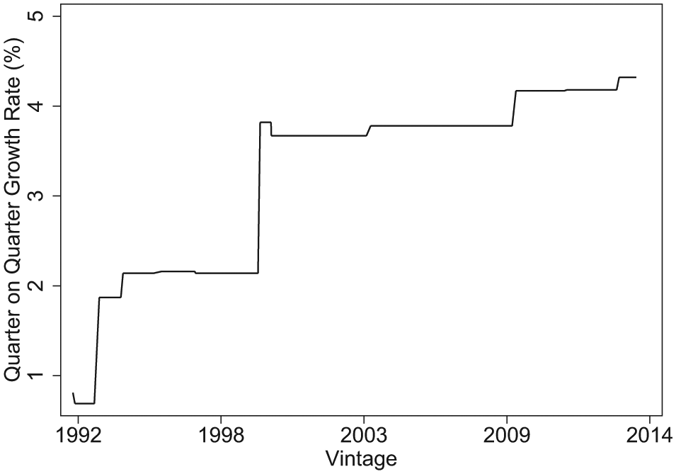
Revisions in Growth Rate Estimate for 1992 Q2. The figure plots all monthly vintages of the quarter-on-quarter growth rate for the second quarter of 1992 since the release of the first estimate in August 1992.
Although revisions in our output growth example from 1992 are larger than most, they are also not extreme outliers. In our data used in the Abramowitz model, for example, the mean absolute deviation for the Q2 on Q1 growth rate from the first estimate released in August of every election year to the 2012 August estimate for all forecasted elections (since 1984) is 1.52 percentage points (with a standard deviation of 1.25). Moreover, revisions in expansions differ substantially from those in recessions (Croushore, 2011: Table 3) and, as noted in the case of real output growth by Stevenson and Duch (2013), changes do not cancel out because of a preponderance of upward revisions.
Making the choice of which data release to use is important for both the theoretical fidelity and empirical performance of a model. Most election forecasts, with the possible exception of James E. Campbell (Campbell, 2008; Campbell and Wink, 1990), ignore the implications of data vintage and simply employ the most recently distributed data vintage, without even being aware that they are making a modeling decision.3,4 If voters indeed respond to the real state of the economy, this decision, though unwitting, is nevertheless correct. If voters respond to media reporting on the initial economic data releases, however, then failing to use “real-time” data to fit forecasting models introduces prediction error and slippage between theory and empirics.
The models
We investigate the effect of data revisions by employing both vintage and real-time data to replicate three prominent forecasting models for US presidential elections and a generic model that we developed, based on findings from Healy and Lenz (2014). The three established models are Lewis-Beck and Tien’s “Core Model”, Abramowitz’s “Time for Change” model and Campbell’s “Trial-Heat” model. To these we add our own “End-Heuristic” model that captures features common to structural forecasting models. All of these models are fit with ordinary least squares (OLS), predict the incumbent share of the two-party vote share and are parsimonious by necessity, as the number of post-WWII presidential elections is small. We collected all data from original sources, so small differences in our results to those presented by the authors of the models might emerge. Election data were obtained from the Office of the Clerk, US House of Representatives; the economic data produced by the BEA were collected from the Federal Reserve’s ALFRED and the Real-Time Data Set for Macroeconomists databases. The first-term incumbent dummy was coded based on the description provided in Abramowitz (2012).
The Lewis-Beck and Tien model is the longest-running that we replicate. The model has changed frequently over the years as Lewis-Beck and Tien (2008) themselves document. We estimate a “core model” that they present in their 2008 article. As with all of the forecasting models that we replicate, Lewis-Beck and Tien use economic growth data as a predictor, which they calculate as change from Q4 of the year before election to Q2 of the election year at annualized rates. The other key predictor is presidential popularity, as measured by the percentage of respondents approving of the job the president is doing in the first Gallup poll in July before the election. For election years for which no early July poll was available we used the poll closest to July that was taken before late August when second quarter economic data became available.
Abramowitz’s “Time for Change” basic model has also undergone revisions. We estimate a basic model from Abramowitz (2012). Thus, as a measure of presidential popularity, we use net presidential approval, the difference between the share of respondents approving and disapproving of the job the president is doing. The approval data are taken from the final Gallup poll in June prior to the election. The growth rate was calculated as annualized change from the first to the second quarter of the election year. We, like Abramowitz, also include a dummy variable coded as 1 if the first-term incumbent ran.
The Campbell “Trial-Heat” model employs two variables: a preference poll and economic growth. Campbell (2012) uses the two-party share for the incumbent from the Gallup preference poll in early September of the election year. Output growth from the first to the second quarter of the election year is the second variable. It is calculated as the difference between the actual growth rate and a “neutral point” growth rate of 2.5% which is divided in half in the case of incumbent party candidates other than the president. From 1992 on, Campbell uses real GNP or GDP.
Our End-Heuristic model captures the features common to most presidential forecasting models in their simplest forms. We use two variables. Presidential popularity is the same measure as used by Lewis-Beck and Tien. Output growth differs from the other models. It is the weighted average of quarterly growth rates in GNP or GDP from the first quarter of the year before the election to the second quarter of the election year. 5 Each quarter receives double the weight of the preceding quarter, which allocates 76% of the overall weight to the election year and 24% to the pre-election year. This approach corresponds to the finding of Healy and Lenz (2014) who find a weight of 3/4 for the election year. 6
Data constraints ruled out two other prominent forecasting models. Fair (1978) employs a larger specification and a longer time series reaching back to 1918, well before the beginning of real-time records. We could re-run Fair’s model using data from 1948 to 2012 but that would leave us with one degree of freedom for our first forecast (1984) and still only eight for our 2012 forecast. Hibbs (2000) uses US military fatalities in foreign wars and a weighted average of real disposable income per capita over the presidential term. Disposable personal income data goes back to 1947 but the only real-time CPI measure that goes back nearly far enough, to 1949, is limited to urban wage earners and clerical workers, i.e. 32% of the population. 7
How accurate are the models that we do replicate? Figure 2 presents the out-of-sample forecasting errors in all presidential elections for all four models. We begin in 1984 both because it is one of the first elections preceded by enough post-WWII elections to support a simple model (1948 is our first observation) and because it was the first presidential election to be de facto forecasted (Lewis-Beck and Rice, 1984). The forecasting models are fit only on observations preceding the predicted election and use the August 2012 economic data vintage. As Figure 2 shows, all four models perform reasonably well.

Four models. Forecasting error (in percentage points) for each model in each election, 1984–2012, i.e. the difference between out-of-sample forecast and election result, for out-of-sample forecasts of the 1984–2012 elections using August 2012 economic data vintage.
Is newer data better data?
Revised economic data presumedly improve the measurement of macroeconomic performance but their predictive validity for voting depends on whether voters respond to the actual state of the economy or to its presentation in the media. Real-time data offer the opportunity to test, if indirectly, the means by which economic voters acquire information about the economy and thereby not only improve theory, but also forecasting and modeling practices. Since real-time data are reported in the media more than revisions, better prediction using real-time (relative to revised) data would suggest that media reporting on the economy influences voters’ economic perceptions. In contrast, if revised vintages perform best, we can infer that voters are most affected by the real state of the economy, likely through direct experience of economic events. Figure 3, using real-time and 2012 vintages, demonstrates that even the growth estimates used in our four forecasting models differ appreciably. Real-time data explain only between 71 and 86 per cent of the variance in 2012-vintage growth data.

Four models, with 2012 vintage plotted against real-time growth estimates. The 45° line indicates perfect correspondence between vintage and real-time estimates. Points above the line indicate that newer estimates have revised growth estimates upwards from the original estimate.
These differences matter for model fit. Table 1 illustrates this with a comparison of point estimates on economic growth when predicting incumbent share of the two-party vote for each of our four forecasting models. Coefficient magnitudes differ by between 6.2 and 17.4 per cent.
OLS model estimates using real-time and 2012 vintage data for each forecasting model. The percentage differences in the Growth coefficients represent the change from the 2012 vintage data to real-time data. The Growth variable is operationalized differently for each of the four models, as explained in Section 3 of the manuscript. Standard errors in parentheses.
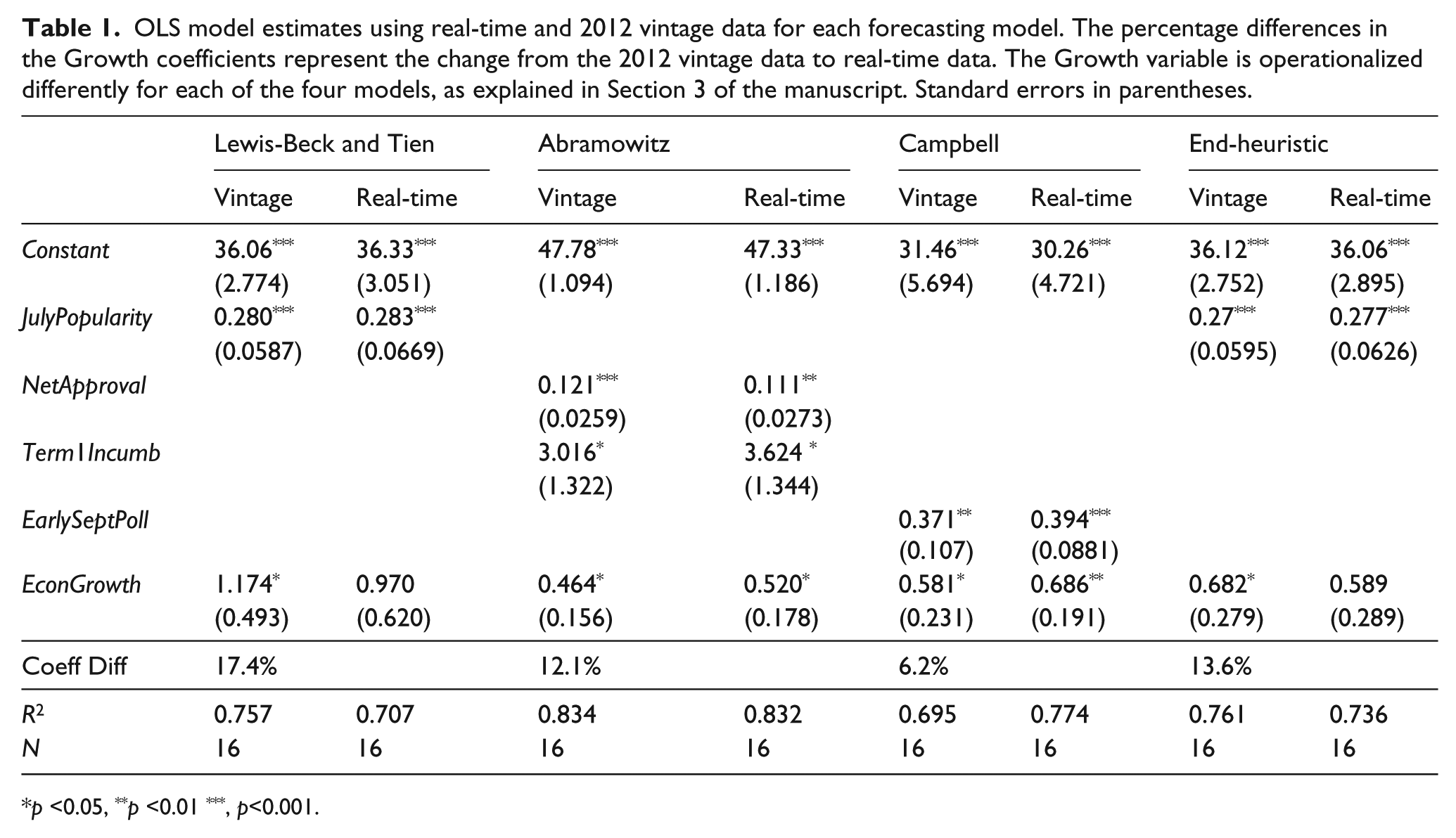
p <0.05, **p <0.01 ***, p<0.001.
We see that initial and revised economic estimates differ and yield subsequent differences in model fit but the question of whether data revisions improve election forecasts remains. By repeatedly forecasting a given election outcome from different data vintages, we should be able to see whether the later vintages improve election forecasts. Figure 4 plots out the absolute prediction errors for all elections since 1984 for each of our forecasting models at each election year since the original. The first forecast for each election uses, of course, real-time growth data available the summer before the election. Each subsequent “forecast” of the same election uses the vintage available at the date of each later forecast. Thus, the plotted point for the 1984 election at the

Absolute forecasting error across different vintages. The first observation in each series represents real-time data.
The results in Figure 4 suggest a positive trend, on average, in absolute prediction error as the number of revisions to a time-series increases. To be more certain and also to estimate the magnitude of any trend, we estimate effect sizes. Table 2 regresses “forecast error deviations”, the difference between each vintage’s absolute forecast error and that from predictions generated with the election year vintage (“most recent vintage”), on vintage number. Since vintage changes also occur in non-election years, we also include years in which no election occurred, up to the most recently available 2014 vintage. By definition, the deviation in vintage year zero (“most recent vintage”) from itself is zero. We specify the model without a constant precisely to fit our regression through the origin, thereby estimating later vintage change from the initial absolute forecasting error.
Deviations in absolute forecasting error from election-year forecasting error as function of data vintage, measured as the number of years since the election. OLS without constant. Standard errors, clustered on election, in parentheses.

p <0.05, **p <0.01 ***, p<0.001.
All four models show a positive effect of data vintage on error size, three of them statistically significant. The Lewis-Beck and Tien model stands out for the size of its effect. Using a data vintage from 10 years after the election results in a forecasting error that is on average four tenths of a percentage point greater than the error obtained when using the vintage available prior to the election. The Abramowitz model, in contrast, finds no effect at all but even here absolute forecasting error increased after the first vintage for all but two elections (1988 and 2004).
Simulated practice
The previous section demonstrated that later vintages introduce greater forecasting error. In practice, however, forecasters follow two conventions that may reduce vintage effects. They usually choose the most recent vintage of economic data for their models. While these data have still undergone revisions since their first release, they have undergone fewer updates than we document above. For this reason, most-recent-vintage data should yield smaller differences from forecasts with real-time data. Moreover, practitioners only use revised data to fit their models but then employ the real-time economic figure for the present election year to calculate their forecast. When considered together, one should expect the difference to shrink further. This section compares real-time forecasts to actual practice.
Consider the choices that researchers, to stick with our example, would likely make in forecasting the 1992 US presidential election. These forecasters, working in the summer of 1992, would obtain the latest vintage of economic data from the BEA or elsewhere and, together with data on presidential popularity and possibly other variables, fit a model. Taking the point estimates from this model, they would then plug in the most recently released popularity and economic growth figures to get their forecast. Their forecast only uses vintage data for fitting the model, not for the second step in which they place the real-time (1992) values in the model to get their forecast. All differences that we observe between forecasts based on real-time data and most-recent-vintage data come from the first step in which the model is fit. When time series are short, as is the case with elections in the 1980s, we expect greater forecasting error simply due to small samples; but we also expect to see little advantage for real-time data since the number of revisions in a short time series is modest.
Table 3 demonstrates this result. 8 We assess the predictive quality of the four models on the basis of multiple synthetic out-of-sample forecasts making forward predictions of election outcomes. We fit each forecasting model for each election with three data vintages: (1) the 2012 vintage, the election year closest to the authorship date of this article; (2) the “most recent vintage”, i.e. that data that an election forecaster would use in each election year when forecasting that year’s election; and (3) real-time data that excludes all revisions. Since we are simulating actual practice with the “most recent vintage” data, we plug (real-time) economic measures from the quarters preceding each election into each fit model, consistent with the model descriptions above, to derive each forecast. Forecasts using the 2012 vintage, in contrast, use the 2012 vintage estimates both for model fit and for the quarters before each election. Real-time forecasts, of course, use real-time estimates for all economic data, for both model fit and forecasting.
Mean errors across models and vintages.
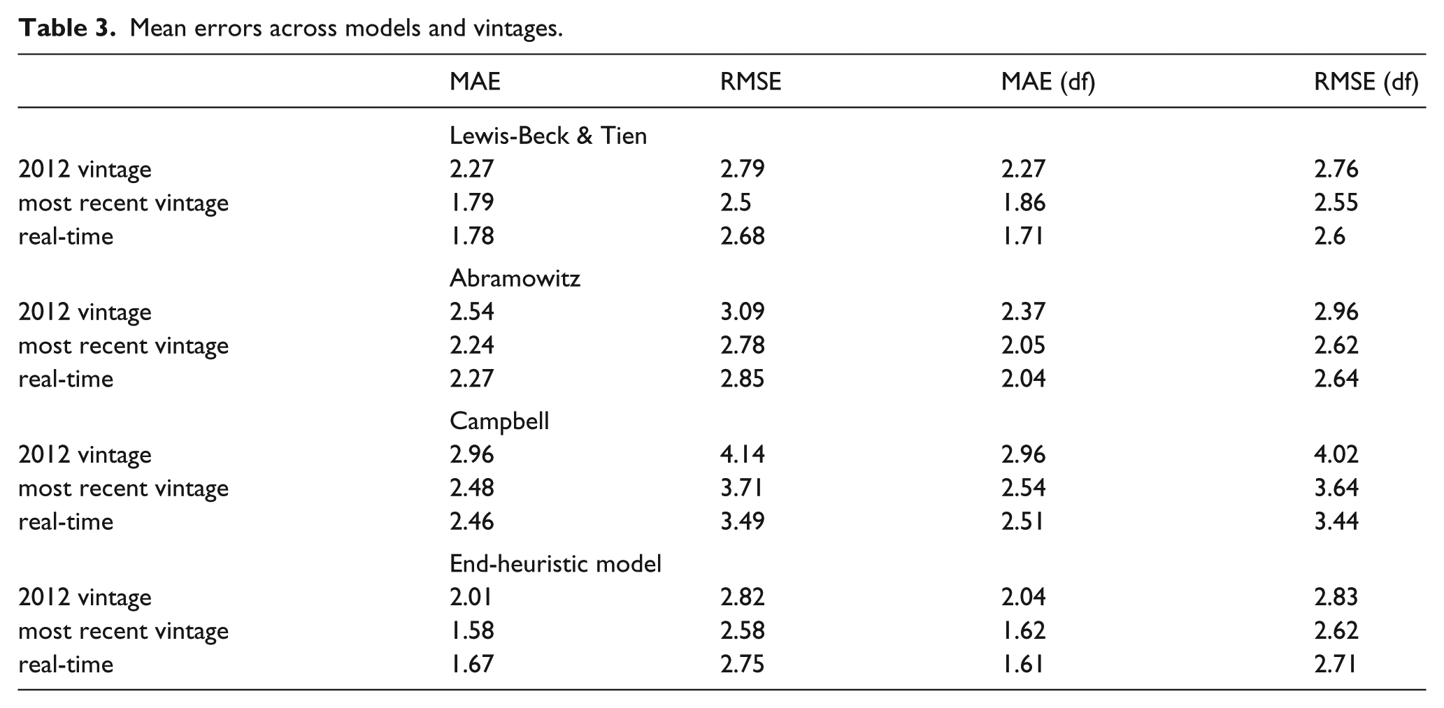
We average the forecasting errors for each type of data for each model across all forecasted elections in four different ways. Table 3 reports the mean absolute error (MAE) and the root mean squared error (RMSE), both unweighted and weighted by degrees of freedom, for all elections, models and types of data. The degrees of freedom (df) weights account for the fact that more recent elections enjoy longer time-series. As expected, forecasting error, regardless of how it is averaged, is systematically larger using the 2012 vintage of economic data. This reflects the fact that the economic measures used for both the model fit and forecast were repeatedly revised. More interestingly, from the perspective of evaluating actual practice, the differences between forecasts based on most recent data vintage and real-time data are much smaller. Indeed, on balance, it is difficult to discern whether one type of data generates smaller forecast errors than the other. Models using growth as the only predictor produce similar results, as shown in Section 6 of the online appendix.
One could interpret these results as an endorsement for the status quo methods of data selection. Such a conclusion, however, might be overly hasty. As time series get longer they should include estimates of economic performance for ever more distant election years with ever more revisions. The absolute deviation between initial output estimates and vintage estimates grows with the number of revisions, as we show in the online appendix. Moreover, these deviations do not cancel each other out with mean revisions tending to be positive (Aruoba, 2008). Estimates of aggregate output increase, on average, by 0.52 per cent between the initial release and the latest available data (Croushore, 2011: p. 81, Table 3). 9 Given that estimates of the economic vote, to take a recent example, associate a one point increase in output with between a 0.8 and 1.4 point increase in the incumbent party vote share (Becher and Donnelly, 2013), deviations of this magnitude can have notable effects in forecast accuracy. Longer time-series with greater deviations from initial economic estimates then suggest increasingly inaccurate forecasting models.
Precisely such a trend appears to be emerging in our models. Figure 5 plots the difference in absolute forecasting errors between the real-time and most-recent vintage, with negative values indicating greater error in forecasts based on most-recent-vintage data. Differences between forecasts based on the two types of data have declined over time. Of greater interest is the trend toward greater forecasting error with most-recent vintage economic data (actual practice) shown as negative values in Figure 5. These results, significant in two of the four models, are too preliminary to be anything more than suggestive. Nevertheless, in precisely those models, the Lewis-Beck and Tien and end-heuristic models, where the result in Table 2 and Figure 4 suggest the largest increase in forecasting error from vintage revisions, we also see the strongest evidence of growing forecast errors with most-recent-vintage data. Section 4 demonstrated that forecast error increases with vintage. Figure 5 suggests that time-series are becoming sufficiently long for these model fitting effects to emerge with most-recent-vintage data.

Real-time versus vintage data: forecasting errors in comparison. Difference in forecasting error between out-of-sample forecasts using election year vintage data and real-time data for elections 1984–2012. Negative values indicate greater error in forecasts based on most-recent-vintage data (actual practice). Regression line based on bivariate OLS model (significant coefficients indicated by solid line).
Conclusion
We have systematically compared the predictions of four forecasting models using real-time and vintage data over numerous presidential elections in the United States. Our results demonstrate that later vintages introduce greater forecasting error and suggest that error magnitude should increase under current forecasting practices as time series get longer and the average number of revisions to the data increases. Although revised macroeconomic data may measure the state of the economy better (Croushore, 2011), they predict electoral outcomes less well. This finding suggests, indirectly, that voters respond more to initial economic estimates, that are heavily reported in the media, than to the economy itself. It also strengthens the argument for subjective economic measures in studies of the economic vote (Stevenson and Duch, 2013). Indeed, we can expect that the effect of data revisions on economic voting results are even greater than those for forecasting. Unlike forecasting with most recent data vintages, which fits the model on vintage data but uses the most recent (i.e. real-time) data for the forecast, economic voting usually only fits vintage data.
We conclude with one broader point about forecasting. We have focused on predictive validity but model stability is also a critical criterion for evaluating a forecasting model over time. Campbell (2014: p.302) argues that an “unchanged and fairly accurate forecasting model should be considered more credible than a one-hit wonder or frequently tweaked model”. Election forecasters frequently change their models, most often by adjusting their measures of presidential approval or of economic growth. The use of vintage data, we argue, raises the likelihood of such model revisions. When a new model outperforms the old model in out-of-sample forecasts of the past election, forecasters are wont to adjust their model. When preparing a new forecast, however, they introduce not only a new observation but a completely new time series. Thus, model changes justified by an improved fit to the “new information”, the new election in the time series, are, in fact, fit on revised economic estimates, muddying the source of any “improvements”.
The implications of data revisions for macroeconomic forecasting have received considerable attention in economics. While economists rely on data revision to improve their economic forecasts, election forecasters and scholars working on the economic vote might be better off ignoring these revisions and using unrevised real-time data.
Footnotes
Acknowledgements
We gratefully acknowledge comments and suggestions by Dirk Ulbricht, Konstantin Kholodilin, Thomas Gschwend and colloquium participants at the Chair for Quantitative Methods in the Social Sciences, University of Mannheim.
Funding
This research received no specific grant from any funding agency in the public, commercial, or not-for-profit sectors.