Sage Journals: Discover world-class research

Abstract

Numerical analysis is increasingly used for batch modelling runs, with each individual model possessing a unique combination of input parameters sampled from a range of potential values. Whilst such an approach can help to develop a comprehensive understanding of the inherent unpredictability and variability of explosive events, or populate training/validation data sets for machine learning approaches, the associated computational expense is relatively high. Furthermore, any given model may share a number of common solution steps with other models in the batch, and simulating all models from birth to termination may result in large amounts of repetition. This paper presents a new branching algorithm that ensures calculation steps are only computed once by identifying when the parameter fields of each model in the batch becomes unique. This enables informed data mapping to take place, leading to a reduction in the required computation time. The branching algorithm is explained using a conceptual walk-through for a batch of 9 models, featuring a blast load acting on a structural panel in 2D. By eliminating repeat steps, approximately 50% of the run time can be saved. This is followed by the development and use of the algorithm in 3D for a practical application involving 20 complex containment structure models. In this instance, a ∼20% reduction in computational costs is achieved.

Keywords

Risk probability computation time data batch

Introduction

Numerical analysis is a vital tool that enables engineers and researchers to investigate diverse phenomena, draw relationships between key parameters, and test scientific hypotheses. In particular, numerical modelling for blast analysis possess significant advantages related to cost, safety and efficiency when compared to conducting practical experiments, which themselves may be impractical or unfeasible given current technological and resource constraints. However, the solution of complex wave propagation problems using physics-based modelling approaches typically requires considerable computational expense and large run times.

Deterministic approaches to blast wave analysis involves a single input pattern being provided to a chosen numerical solver, with a single set of values being output. Considering the unpredictable nature of explosive events where the size, shape, material and position of the explosive charge cannot be known before the detonation takes place, this approach to modelling risks the possibility of misrepresenting the threat posed to a given structure or its inhabitants. Probabilistic approaches are therefore becoming more prevalent in blast protection research and design (e.g. Qi et al., 2020; Seisson et al., 2020; Rebelo and Cismasiu, 2021) as they enable the analysis of a large number of randomly generated model inputs with additional consideration for modelling errors (Stewart et al., 2006; Stewart and Netherton, 2015). Use of Monte-Carlo sampling of the input variables means that randomly selected explosive events are simulated based on the predefined possibilities of each parameter (Murmu et al., 2018). Therefore, instead of being provided with a single output, with this approach the user obtains probability distributions of each tracked variable that can be used to assess the risk to a higher fidelity.

Despite these benefits, probabilistic studies still require a deterministic model to provide the results for every input combination. Accordingly, when analysing complex scenarios, computational fluid dynamics (CFD) solvers could produce total computation times beyond what is acceptable. This is highlighted in a study by Alterman et al. (2019), where 1.55 hours was required for each of the 100 models that were used to determine the fatality risks of a specific domain. There is therefore a clear need for tools that are more suited to the rapid analysis of complex explosive events.

Machine learning (ML) approaches offer the opportunity for such a reduction in run time, however training and validation processes require large amounts of high quality data, which is often generated entirely (or at least supplemented by) numerical modelling results, (e.g. Bortolan Neto et al., 2020). Thus, generation of the database itself brings a significant capital investment in computation time. For example, in a recent study by the current authors (Dennis et al., 2021), an Artificial Neural Network (ANN) was trained to predict blast loading distributions within a confined space to a reasonable level of accuracy (±10%), with results for the whole domain being generated in less than 4 minutes. Achieving this performance required 72 individual numerical analyses to populate the training/validation data set, each requiring around 2 hours of computation. The benefit of developing a fast running ANN is clearly offset by this initial investment, highlighting how the reliance on computationally expensive numerical models remains a key issue.

This requirement for accurate yet rapid computational calculation methods has driven many developments in recent years. One particular example is adaptive mesh refinement (AMR) (Berger, 1989; Belhamadia et al., 2014), where areas of the computational domain are refined at a local level, allowing for coarser representation elsewhere and therefore significant computational savings. A remaining issue, however, is that if a new scenario needs to be simulated, the entire process needs to be remodelled, regardless of any areas of commonality with previous simulations. The focus of this study is therefore to develop a robust and reliable method for systematically identifying and removing any duplicate steps in a batch of numerical models, with the potential for significant time savings in both probabilistic studies and in the development of machine learning datasets.

The ‘Branching Algorithm’ is introduced in this article as a tool for batch analyses that identifies the points/times where the parameter field of each arrangement would become unique to its domain. It was initially created as a method that could be adapted for a range of numerical problems and so a generalised mathematical representation of the algorithm is provided in Appendix A. By operating at a batch-level as opposed to a model-level, as with AMR, the algorithm produces an informed data mapping framework (deviation tree) that can be evaluated in a suitable numerical solver to ensure that duplicate steps are only calculated once in each batch of tests.

The following sections discuss how the algorithm operates and is suited to blast analyses in both 2D and 3D, with a walk-through of the proposed method being applied to a simple 2D batch of blast panel models also being presented to show that approximately half the time steps, and therefore half the computation time, can be removed through informed data mapping. This is followed by a more complex set of 3D containment models, where around 20% of the computation time is identified as obsolete. The work presented in this article shows that, for time-dependant simulations, a significant computational saving can be expected when using the proposed method compared to when each model is ran from birth to termination with no consideration of the test similarities.

The branching algorithm

Principles and terminology

Time-varying numerical forward models can be used to estimate a parameter field, θ, given initial conditions, Ω, in some domain, Δ. The parameter field could, for example, include pressure, temperature and stress at each specified point and it could be used to assess the impact of an explosive, development of a crack, or variation in any relevant quantity. With the aim of the proposed algorithm being to avoid duplicate calculation steps in a batch simulation process, consideration of how the parameter field, θ, changes with respect to space and time in each given domain is required. The calculated parameter field at a location given by x, y and z, at time, t, is therefore given by equation (1), with f(⋅) representing the given numerical model.

θ_{t} (x, y, z) = f (x, y, z, Ω, Δ, t, θ_{t - 1})

(1)

Provided that multiple models are compatible for data mapping according to a user defined subset of the input conditions, χ, it is possible for the branching algorithm to define a ‘trunk model’, given by Δ^T, Ω^T and θ^T, that corresponds to the test arrangement that simulates a developing parameter field that is common to all other models relative to a specific domain location up to a certain time step.

The specific time step when the trunk model and any other given model (or ‘branch’ of models) from the batch of tests stops producing identical parameter fields can be defined as the ‘deviation point’ for that model. This is given by equation (2), with $θ_{t}^{T} {(x, y, z)}_{r}$ representing the trunk model’s parameter field at time step, t, in a position given by the relative x, y and z coordinates. Similarly, $θ_{t}^{n} {(x, y, z)}_{r}$ denotes the parameter field at the same relative location and time step, in model n of the batch.

θ_{t}^{n} {(x, y, z)}_{r} \neq θ_{t}^{T} {(x, y, z)}_{r}

(2)

The relative position in the domain is given by equation (3):

{(x, y, z)}_{r} = {(X, Y, Z)}_{r} - (x, y, z)

(3)

with

\begin{array}{l} (x, y, z) = Position of the point in model n' s domain \\ {(X, Y, Z)}_{r} = Relative point that is common between both models, n and T \end{array}

The comparison between the trunk model’s state,

θ_{t}^{T}

, and any other model at the same time step,

θ_{t}^{n}

, is only possible if the relative domain location is shared as this removes the influence of varying domain shapes and sizes. For example, comparing multiple domains that are modelling an explosion requires the shared location to be at the detonation point of the explosive as this is the initiation point that causes changes to the parameter field in the surrounding area.

Further, a deviation point corresponds to the first time step where the model’s calculated parameter field would be different from the trunk model. Mapping the data associated to $θ_{t - 1}^{T}$ to the new domain for use with its own input and domain conditions, Δⁿ and Ωⁿ, with (X,Y,Z)_r acting as the origin, therefore enables simulation steps in model n from t = 0 to the current mapping time to be saved.

The branching algorithm determines the deviation point with respect to the spatial location, (x, y, z), for each model prior to any numerical simulation by assessing the ‘influences’ present in each domain. These influences are defined as the factors that change the input conditions into the observed outputs, meaning they are bespoke to each potential application of the algorithm. However, they will be defined by a subset of the inputs to the numerical calculation:

λ_{i}^{n} \subset [{(x, y, z)}_{r}, Ω^{n}]

(4)

where i is the influence number. Example influences include specific boundary constraints, time-dependant calculation variables, or possibly entire calculation methods that are introduced after a threshold value is reached.

In order for the algorithm to discern when each influence is reached in each respective model, a comparison metric, γ, is defined for all entries. The time step associated with when each potential deviation is reached in the numerical model may not be known prior to the simulation of each domain; however, an expected sequence of when each point is met can be defined with consideration of additional parameters. Again, for the example of modelling an explosion, the distance/time that the blast wave will travel before it will reach each influence can be used to define the order of influence activation, therefore allowing the algorithm to identify if there are any deviating simulations.

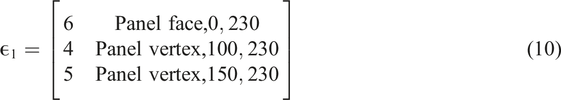
The selected influence that correlates to the deviation point of a given model is provided as the output to the algorithm in an ordered vector denoted by ϵ. Here, ϵ provides the deviation condition and the associated model number in a list that is sorted according to when each entry is reached in the trunk model’s simulation. For example:

ϵ = [\begin{matrix} 1 & λ_{3}^{1} \\ 4 & λ_{2}^{4} \\ \dots & \dots \end{matrix}]

(5)

This shows that model 1 is the first to deviate from the trunk, due to the influence defined by

λ_{3}^{1}

. Model 4 follows this due to a deviation at its second influence,

λ_{2}^{4}

As the parameter field of the trunk model, θ^T, undergoes a change that is not expected to be present in the model given by ϵ₁(n), the latter should be initiated by data that is mapped from the last time step of the trunk model. The deviation condition given by ϵ₁(λ) is used to identify when this will occur. Once mapping to this domain has taken place, the trunk model simulation continues until the condition defined by ϵ₂(λ) is met, and another phase of data mapping can take place. This process continues until all compatible models have been initialised as shown in Algorithm 1 provided in Appendix A.

The branching algorithm for blast analysis

Adapting the methodology explained in the previous section for use with blast analyses requires the key terminology to be assigned to blast relevant parameters. Notably, a deviation point is provided in terms of its spatial location relative to the charge, since the air that fills the domain will remain at ambient conditions until the blast wave emanating from the explosive material reaches that particular point. The solutions to each model will therefore diverge at the moment that the pressure wave reaches a location or material in a given domain that is not present in the other models. The influences used to identify these locations can then be associated to object or boundary surfaces, or changing material properties.

For the branching algorithm to allow for data to be mapped between various models, it is essential for some of the input conditions to be identical. For blast analyses, this relates to the ambient conditions of each domain and the charge shape and composition. If there is a difference between two models because of these variables, the simulation would be different from birth and so no mapping would be possible. The algorithm therefore splits models of a batch into various trees that are sorted and analysed separately. The size of the charges used in each model will not necessarily be a reason for defining a new deviation tree as domain scaling can be used according to Hopkinson-Cranz scaling laws (Hopkinson, 1915; Cranz, 1926). Use of this approach improves the compatibility of models because each domain in the batch of tests can be defined in terms of scaled distance, with a single charge size relating all arrangements. However, for the examples given by this study, scaling was not required.

A simplified version of the blast branching algorithm is provided below to show how the comparison of each domain allows for informed data mapping to take place.

1. Identify unique geometries and create discrete influences associated to the objects and boundaries for each model.

2. Identify the groups of models (deviation trees) that can share numerical data with no loss of modelling accuracy by considering the probabilistic inputs being used (e.g. separate groups are required for differing charge shapes and/or ambient conditions as data mapping cannot occur if difference are present from birth of the simulations).

3. For each tree:

(a) Calculate the wave travel distance to each influence of each model so that comparisons between influences can be made.

(b) Compile all influences and identify which model has the unique influence that is the furthest distance from its charge. This model acts as the ‘trunk model’, with all other models deviating from its solution.

(c) Remove influences that are common between the trunk model and any others. Sort the remaining influences from all models so that the first entry is the one that is closest to its respective charge.

(d) Take the first entry as the first deviation from the trunk model and remove any other influences associated to this model from the remaining influence store. Continue this process until all models have deviated.

(e) If multiple models share the same deviation at any point, a ‘sub-trunk model’ can be defined by repeating the process with this sub-set of models to allow for additional savings and multiple informed data mappings.

Ultimately, with the model geometries, boundary and ambient conditions and charge characteristics being defined as the input values, this process automatically produces a modelling order for a batch of tests. Through generating a number of deviation locations based on the blast wave’s progression through the domain of a parent model (trunk or sub-trunk), the chosen numerical solver can be monitored so that data maps are created just before the trunk model’s parameter field diverges from that of a branching model. The associated branching models can then be initialised with the exported data maps, removing the need for repeated calculations to be computed, specifically around the charge before the blast wave impacts any boundaries or surfaces.

An example of a deviation tree being output from the algorithm is provided by Figure 1 with model ‘N’ being assigned as the trunk model and various branches showing where data mapping can be utilised. It is also shown how model ‘N-1’ is defined as a sub-trunk model, meaning models ‘N-1’, ‘N-3’ and ‘N-4’ were all identified to deviate from model ‘N’ at the same influence. Additional repeated simulation steps were then identified in a second pass through the branching algorithm when considering only these three models. The recursion capability of the algorithm is therefore essential in allowing for the greatest computational time saving.

Figure 1.

Example deviation tree obtained using the branching algorithm.

After application of the branching algorithm, a tool capable of performing analysis of the branched network of models will be required. It is important to ensure that there is no/limited detrimental impact to the progressive accuracy of the solutions as data is transferred from one model to another. It is not expected that this would be a problem for many modelling techniques as studies adopting methods such as domain decomposition, multigrid solving and mesh adaptation are able to efficiently solve highly complex problems with data being transferred between parallel computing processors many times throughout the simulation (Wu and Tseng, 2005; Bruneau and Khadra, 2016; Park and Kwon, 2005).

This introduction to the branching algorithm aims to provide a basic understanding of the logical process being employed by the proposed method; however, the following section will expand on this for 2D blast simulations with a walk-through of how the influences are identified and compared.

Example application in 2D

Problem scenario

To show that the proposed algorithm and simulation strategy can be highly beneficial in saving computation time, a batch of nine 2D models based on the experimental work presented by Rigby et al. (2018) and Rigby et al. (2020) have been simulated using the proposed method. Simulation times will be compared between the branching algorithm method and a standard birth to termination approach for the same nine models, with all other factors being identical (mesh size, computational resource, etc.).

In the aforementioned experimental work, tests were performed using a 100 g spherical PE4 charge positioned 80 mm and 380 mm from a rigid target. The results were then used to validate the numerical solver LS-DYNA for use in modelling near-field explosions. Expanding upon this framework, Table 1 gives additional scenarios that may be explored, with varied charge locations providing three distinct stand-off distances; 80, 230 and 380 mm for three different target blast panels diameters; 200, 300 and 400 mm. As shown in Figure 2, the panels are assumed to be rigid with a constant thickness of 50 mm in a domain that features non-reflecting, ambient boundaries (aside from the axis of symmetry that enables these problems to be considered in 2D half-space). The charge size, shape and material also remain consistent in all cases.

Table 1.

Model setup parameters.

Model No.	Panel diameter (mm)	Charge stand-off (mm)	Charge size (g)	Charge material and shape
1	200	80	100	PE4 sphere
2	300
3	400
4	200	230
5	300
6	400
7	200	380
8	300
9	400

Figure 2.

Explosive test arrangements to be used with the branching algorithm shown in 2D. Charge is given as a red circle and the impacted panel is shown in grey. Boundaries are ambient non-reflecting. Model numbers are provided in the lower right corner of each image. All dimensions are in millimetres.

Validation of LS-DYNA for blast analysis

The experimental results first published in Rigby et al. (2018) are used to validate the use of LS-DYNA in this article. The detonation of a spherical 100 g PE4 charge placed 80 mm from the rigid plate is simulated using LS-DYNA’s multi-material Arbitrary Lagrangian Eulerian (MMALE) solver. This allows each cell in the model domain to contain air and high explosive without either material needing to coincide with the cell boundaries (Peery and Carroll, 2000) and it is therefore capable of simulating explosive scenarios. Values assigned to each of the relevant material model and equation of state parameters are provided by Rigby et al. (2018).

It is essential for the progression of the blast wave that the initial energy is preserved throughout the detonation process (Lapoujade et al., 2010) and generally over 10 elements across the radius of the charge should be used to ensure sufficient accuracy of the detonation (Schwer and Rigby, 2018). The use of 1.25 mm square elements provides ∼20 elements across the radius of the charge and is deemed acceptable in this instance. Figure 3 shows a comparison on the numerical and experimental reflected pressure and specific impulse (cumulative temporal integral of pressure) histories at the centre of the target panel (0 mm), 50 mm away and 100 mm away from the centre. Furthermore, Table 2 provides the peak values from these plots to verify that the magnitudes and general form of the profiles are in reasonable agreement, giving confidence in the ability of the numerical approach to adequately simulate the salient physical processes.

Figure 3.

Pressure-time and specific impulse-time histories for the detonation of a 100 g PE4 charge placed 80 mm from a rigid plate for three distances from the centre of the plate.

Table 2.

Peak reflected pressure and specific impulse values from the experiment and simulation profiles shown in Figure 3.

Distance from plate centre (mm)	Peak reflected pressure (MPa)		Peak specific impulse (MPa.ms)
Distance from plate centre (mm)	Experiment	Simulation	Experiment	Simulation
0	209.08	256.92	3.87	4.01
50	107.78	146.73	1.96	1.45
100	42.03	43.22	0.65	0.66

The discrepancies between experimental measurements and numerical output have been seen previously Rigby et al. (2018), and are likely attributed to the strong directionality, high pressure/velocity gradients and magnitudes of the near-field blast. Whilst they appear significant when viewing discrete pressure and impulse histories, they are less significant for target response considerations due to the relatively low areas over which they are acting (compared to the pressure histories at 100 mm from the centre which demonstrate much better agreement).

It is likely that a smaller element size would provide an improvement to the agreement in all pressure and impulse profiles; however, the use of 1.25 mm elements ensures a balance between accuracy and computation time will be achieved in the following analyses.

Model specification

Following the successfully validation of LS-DYNA with 1.25 mm elements, each scenario in the example batch of tests given by Table 1 and Figure 2 is modelled using this mesh density and the same material model and equation of state parameters provided by Rigby et al. (2018). They are also modelled in 2D axi-symmetry with the domain boundaries being defined at distances that are sufficiently large so that although reflections will occur as the shock waves impact the boundary nodes, the returning shock waves will not reach the panel before the termination time is met.

As shown in Figure 4, models 1, 2 and 3 were simulated in a 350 × 230 mm domain, with the panel positioned with y-coordinates of 160 mm and 210 mm. Models 4, 5 and 6 were simulated in a 350 × 380 mm domain, with the panel positioned with y-coordinates of 310 mm and 360 mm. Finally, models 7, 8 and 9 were simulated in a 350 × 530 mm domain, with the panel positioned with y-coordinates of 460 mm and 510 mm.

Figure 4.

Numerical models showing the various stand-off distances, blast panel diameters (grey rectangle) and the 49.2 mm diameter charge (red semicircle). (a) Models 1, 2 and 3 (b) Models 4, 5 and 6 (c) Models 7, 8 and 9.

The termination times for models 1, 2 and 3 were then set at 0.12 ms, models 4, 5 and 6 at 0.2 ms and 7, 8 and 9 at 0.28 ms. This allows for the initial blast wave to fully clear the panel without interference from any unwanted reflections.

In every instance, the charge is centred with a y-coordinate of 80 mm so that the data mapping, achieved using the *initial_ale_mapping keyword (Aquelet and Souli, 2008), was implemented relative to a consistent point in all domains. Furthermore, since the panel dimensions and its location coincides well with the element mesh of each domain, it is modelled by fully restraining the elements that fall within the respective geometry. This has the effect of creating a rigid reflecting surface and it removes the need to create a new part and material type in the LS-DYNA model.

Algorithm walk-through and output

With the model geometries clearly defined, the branching algorithm can be used to identify the deviation points where the numerical outputs from each simulation will cease being identical. This section will step through the key stages of the algorithm to show how it systematically selects when each model should be initiated with data mapped from the trunk model.

It is to be noted that this walk-through ignores the complexity that may be required for other applications or in use with more detailed test scenarios. For example, the panels are assumed to be rigid, that is, any motion of the panel following application of the blast loading occurs on timescales such that the development of loading is itself unaffected. This has been shown to be a reasonable assumption when considering blast loading on structural panels (Rigby et al., 2019). Each model is also being solved with the same method, ambient conditions, charge material/detonation location and panel properties, and therefore it is only the differing domain geometries that will provide diverging solutions. This also allows influences to be stored with their spatial locations and comparison values only, as the material properties and surface slopes will not lead to deviations. In the next example application, the 3D problems require a more comprehensive set of variables to be stored to enable influence comparisons to be made correctly.

By entering the geometry and charge location in Figure 2 into the branching algorithm, the influences associated to rigid object and boundary vertices and faces can be defined as shown in Table 3. Here the coordinates of the key points on the panel relative to the charge are used to define the influences themselves (columns 3 and 4). These are then assigned a comparison value (γ) that enables the algorithm to sort when each influence will be reached in a numerical simulation. For this example, γ is equal to the direct distance between the charge and the identified point (column 5). This value would ideally be assigned to the arrival time of the blast wave at each location; however, for simplicity the distance measure is used. It is at this stage where any influences that are present in all models would be removed if required.

Table 3.

Individual influences for each model being considered are formalised in the influence table below. Rear nodes of the panels are omitted for brevity. Influence defining the trunk model is shown in italics.

Model No.	Influence Location	Relative x coordinate (mm)	Relative y coordinate (mm)	Distance from charge centre, γ (mm, 0 d.p)
1	Panel face	0	80	80
1	Panel vertex	100	80	128
2	Panel face	0	80	80
2	Panel vertex	150	80	170
3	Panel face	0	80	80
3	Panel vertex	200	80	215
4	Panel face	0	230	230
4	Panel vertex	100	230	251
5	Panel face	0	230	230
5	Panel vertex	150	230	275
6	Panel face	0	230	230
6	Panel vertex	200	230	305
7	Panel face	0	380	380
7	Panel vertex	100	380	393
8	Panel face	0	380	380
8	Panel vertex	150	380	409
9	Panel face	0	380	380
9	Panel vertex	200	380	429

Next, the trunk model can be defined by finding the model that encounters its first unique influence at the latest calculation step in its respective domain. This ‘greatest unique initial influence’ corresponds to the test arrangement that will see all other models deviate from its solution before the step where it would have deviated from the other models itself, thus enabling the largest number of duplicated steps to be removed from each simulation process.

By assessing Table 3, it can be seen that model 9 will be the trunk model since its first unique influence corresponds to the blast wave impacting the panel vertices at the greatest distance from the charge; 429 mm. The influences present in this newly-defined trunk model can then be removed from all other model’s tables, provided that they would occur at identical locations within each simulation. For this example, this relates to the panel face impacts for models 7 and 8, since columns 3, 4 and 5 of Table 3 contain identical values.

Following this step, a combined table of influences is formed (Table 4) and ordered according to the direct distance from the charge. The first entry therefore corresponds to the first model that deviates from the trunk (i.e. the model that reaches an influence causing the output of the simulation to diverge first). As the algorithm works though the table of remaining influences, any model that deviates from the trunk has its entries removed. The order of when each model deviates can therefore progress to each model in the batch of tests until no entries remain.

Table 4.

Combined influence table is formed and sorted according to the time when each entry is encountered by the blast wave. Entries included in the trunk model are removed.

Model No.	Influence Location	Relative x coordinate (mm)	Relative y coordinate (mm)	Distance from charge centre, γ (mm, 0 d.p.)
1	Panel face	0	80	80
2	Panel face	0	80	80
3	Panel face	0	80	80
1	Panel vertex	100	80	128
2	Panel vertex	150	80	170
3	Panel vertex	200	80	215
4	Panel face	0	230	230
5	Panel face	0	230	230
6	Panel face	0	230	230
4	Panel vertex	100	230	251
5	Panel vertex	150	230	275
6	Panel vertex	200	230	305
7	Panel vertex	100	380	393
8	Panel vertex	150	380	409

For this example, the first deviating model (1) diverges due to an influence that is also present in two other models (2 and 3). It is therefore essential for the algorithm to compare the influence causing model 1 to deviate with the next entries to check if a sub-trunk model can be defined. This allows the algorithm to identify further mapping opportunities that can save additional computation time by removing duplicate steps that occur after the initial mapping from the trunk model.

Removing the influences associated with these three diverging models shows that the second divergence from the trunk model also features three models. Models 4, 5 and 6 are shown to have identical influences for when the blast wave hits the panel at a 230 mm stand off distance. After these have branched off from the trunk model, models 7 and 8 remain, with their relative deviation conditions then being defined by the blast wave reaching the vertices of the panels that are positioned at the same stand-off distance as in the trunk model.

Since two sub-trunks will be required, the branching algorithm utilises recursion and is repeated for the smaller batches of models that deviated from the trunk model at the same point. Table 5 shows the relevant remaining influences for models 1, 2 and 3, with model 3 being defined as the sub-trunk model. It is clear to see how model 1 will deviate first, as the blast wave reaches its panel vertex. This will occur before model 2 deviates for the same reason, at its panel vertex that is slightly further from the charge. The process for models 4, 5 and 6 progresses in a similar way to this example, with model 6 acting as the sub-trunk due to it having the widest panel in its configuration. Model 5 then follows model 4 as the next to deviate. It is worth noting that if multiple models within this sub-trunk had an identical plate diameter but, say, different plate thicknesses, then recursion would be used again to sort those models according to the additional influence relating to plate thickness.

Table 5.

Combined influence table for the first sub-trunk. Model 3 is deemed to be the sub-trunk model.

Model No.	Influence Location	Relative x coordinate (mm)	Relative y coordinate (mm)	Distance from charge centre, γ (mm, 0 d.p.)
1	Panel vertex	100	80	128
2	Panel vertex	150	80	170
3	Panel vertex	200	80	215

According to the sorting process employed by the branching algorithm, the output vector for this tree denoted by ϵ is given by:

ϵ = [\begin{matrix} Model number & Influence causing deviation \end{matrix}] = [\begin{matrix} n & λ_{i}^{n} \end{matrix}]

(6)

Where the influence number, i, causing deviation for model, n, is defined as:

λ_{i}^{n} = [\begin{matrix} Influence location & Relative x coordinate & Relative y coordinate \end{matrix}]

(7)

This results in the output for this example being equivalent to:

ϵ = [\begin{matrix} ϵ_{1} \\ ϵ_{2} \\ 7 Panel vertex, 100,380 \\ 8 Panel vertex, 150,380 \end{matrix}]

(8)

with,

ϵ_{1} = [\begin{matrix} 3 & Panel face, 0,80 \\ 1 & Panel vertex, 100,80 \\ 2 & Panel vertex, 150,80 \end{matrix}]

(9)

ϵ_{1} = [\begin{matrix} 6 & Panel face, 0,230 \\ 4 & Panel vertex, 100,230 \\ 5 & Panel vertex, 150,230 \end{matrix}]

(10)

Figure 5 presents these outputs in the form of a flow chart (a), and deviation tree (b) to show how the trunk model data can be mapped to various domains at the simulation step prior to when there is a change in the ambient conditions at the given locations.

Figure 5.

Algorithm output (a) flow chart, (b) deviation tree. Coordinates given in (a) are given in millimetres to indicate where the model will deviate relative to the charge centre in each model.

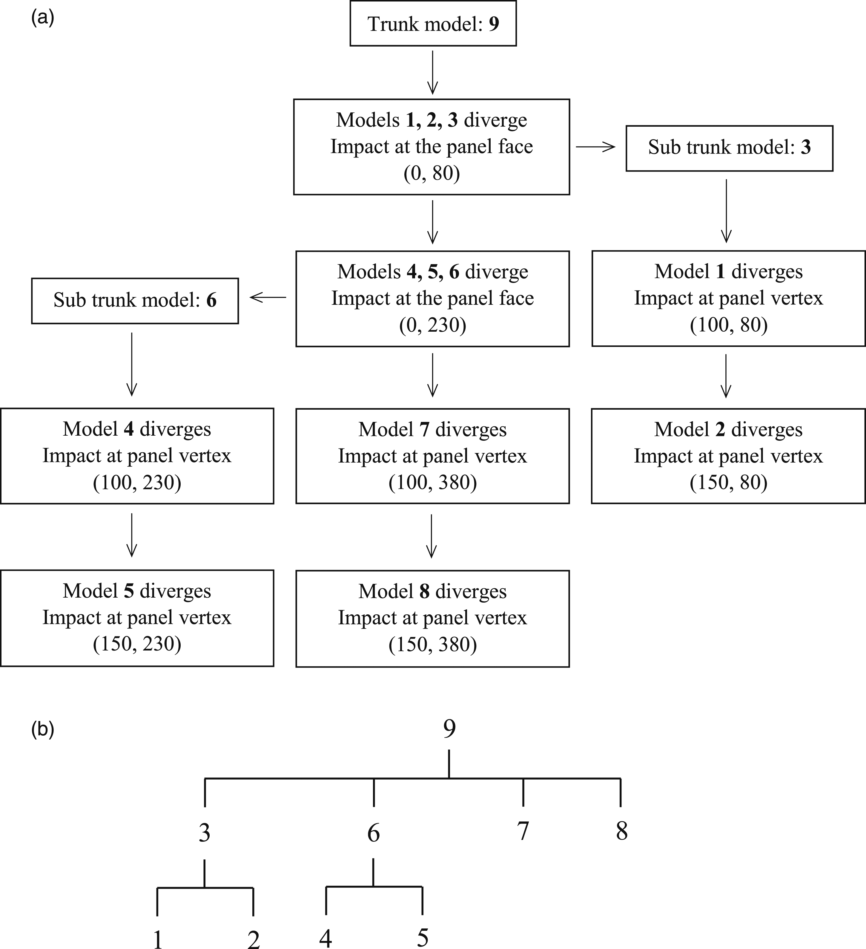
As discussed, the recursion capabilities of the method are highlighted by how ϵ₁ and ϵ₂ present the output from additional passes through the branching algorithm for the sets of models that deviated from the trunk model at an identical influence. This process could occur any number of times to meet the requirements of the models being simulated, with the possibility of sub-sub-trunk models and beyond being identified as discussed above with regards to additional parameters such as plate thickness. Thus, the level of recursion is intimately linked to the number of unique input variables of a batch of numerical models.

Simulation times

With the progression of the models through the algorithm now complete, the order of branching and the corresponding influences causing deviation can be implemented using the relevant solving software to enable an efficient simulation process.

Table 6 shows that when simulating all 9 models in LS-DYNA, the required computation time is 1643 s (27 min 23 s). Use of the branching algorithm and the simulation order shown in Figure 5 reduces this to only 847 s (14 min 7 s), a saving of approximately 50% (13 min 16 s; 48.4%). The reported simulation times were achieved with each model being solved one after another on an Intel Core i7-10700 2.9 GHz processor with 16 GB of RAM. It should be noted that the magnitude of the achieved benefit can be expected to vary greatly depending on the similarities and complexity of the models specified in the batch of tests. However, this basic example still proves that simulation efficiency can be enhanced with the use of the proposed method.

Table 6.

Required computation time for each model with and without use of the branching algorithm method.

Model No.	1	2	3	4	5	6	7	8	9
No branching (s)	90	90	88	173	171	175	284	283	289
With branching (s)	55	49	73	74	70	100	72	65	289
Saving (s)	35	41	15	99	101	75	212	218	0
Saving (%)	38.9	45.6	17.0	57.2	59.1	42.9	74.6	77.0	–
Algorithm computation time:						1 s
Standard method computation time:						1643 s
Branched method computation time (inc. algorithm):						848 s
Total saving (inc. algorithm):						48.4%

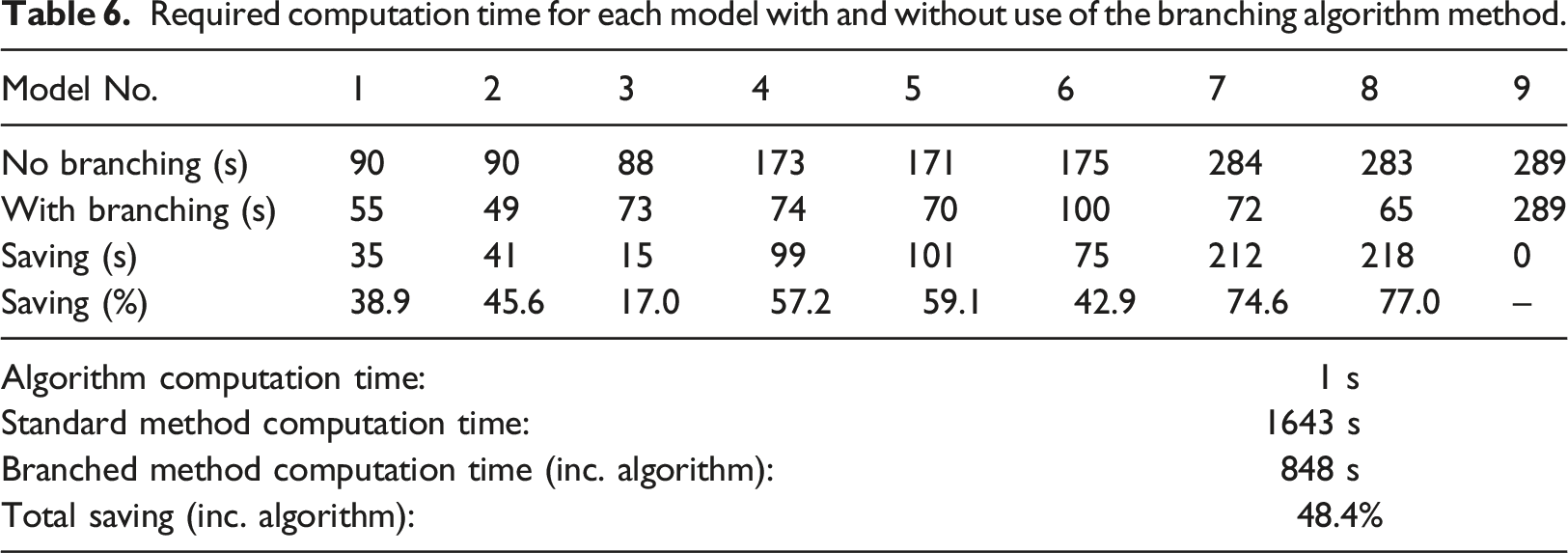
As expected, Table 6 also shows that when using the branching algorithm, models 7 and 8 experience the greatest reduction in required computation time (75–77%) due to how the deviation points occur at later stages of the time-stepped solutions. A larger amount of the trunk model (9) can be simulated without a difference in output for these cases when compared to models 1, 2 and 3 that must diverge as soon as the shock wave has progressed 80 mm from the charge. This is why the branching algorithm works to identify the trunk model by assessing which model from the framework has the unique initial influence that occurs at the latest time step of the simulation.

For a visual representation at how the data is mapped between each domain, Figures 6 and 7 show how the progression of the blast wave occurs in each domain, with the faded images relating to steps that are omitted from the analysis if the branching algorithm is used. These figures also highlight the importance of using the charge centre as a coordinate that is shared between each model since the blast wave can be mapped relative to this point regardless of the domain size and shape.

Figure 6.

Progression of the shock front from the LS-DYNA models showing where data mapping occurs. Faded cells show the simulation steps that are not required if the branching algorithm is used. Data mapping is shown with black arrows.

Figure 7.

Continuation of Figure 6. Progression of the shock front from the LS-DYNA models showing where data mapping occurs. Faded cells show the simulation steps that are not required if the branching algorithm is used. Data mapping is shown with black arrows.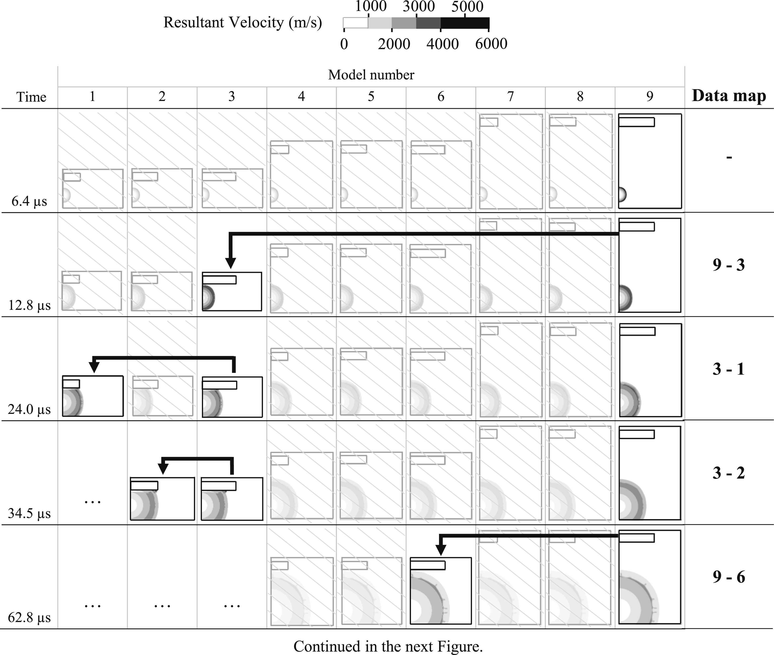

Mapping results

The mapping functionality in many numerical solvers is intended to allow for adaptive mesh refinement where dense grids of elements and nodes need to be specified for the start of a simulation where more detail in the parameter field may be required to preserve the energy of the detonation. When this stage of the process has concluded, the data can be mapped to the same domain geometry, but with a coarser mesh that helps to reduce computation time. Consequently, the mapping process requires interpolation of values to fit to the new mesh.

For the mapping displayed in this article, every model shares the same mesh conditions and so interpolation is not required. This results in rapid initialisation of the models receiving the parameter field from a trunk or sub-trunk model with no loss of information that could lead to differing outputs between a mapped and non-mapped solution.

Figure 8 shows this to be the case with results from the branched analysis being compared to those from the full simulations for model 1. The combined outputs from each stage of the mapping procedure are shown using different line types, with the results from the full simulation shown with a solid black line and mapping times shown as black dashed vertical markers. The results are effectively indistinguishable, demonstrating that the branching algorithm has successfully identified a robust and repeatable methodology for removing unnecessary steps in the simulations.

Figure 8.

Pressure time histories for model 1 generated from simulations with and without use of the branching algorithm.

Developments for 3D analyses

So far this article has proved the concept of the branching algorithm for a tailored example in 2D. The process involved in obtaining the ∼50% computation time saving discussed previously is simplified greatly by using 2D models, making it well suited to a walk-through example. However, the following sections will now explore the developments required in defining and sorting influences present in 3D blast models. This will be followed by a practical application for the simulation of a batch of containment structures.

Domain discretisation and influence comparison

The most important adaptation to make to the branching for use in 3D is related to the definition of the influences in the blast domains. As shown in the previous example and in Figure 9, 2D models only require the object vertices and a single surface definition to be identified as potential locations where the output between different models may diverge. This is because if the wave hits the surface, the next point it will hit is a vertex and vice versa. Conversely, in a 3D model, the label ‘edge’ is required since the wave can progress in multiple directions and its impact at the edges may lead to deviating outputs.

Figure 9.

Comparison of how a blast wave may interact with a rigid object in 2D and 3D.

With this inclusion, the way in which the algorithm identifies and compares influences must change to account for variations in the type of impact the wave is predicted to experience. Specifically, in order for the branching algorithm to identify which parts of a given domain are reached first, potentially causing a deviation, the geometries of each model must be represented discretely. This requires a series of nodes to be defined to act as individual influences on all surfaces of the objects and boundaries and along all edges in each domain.

The mesh of influences representing each object and boundary surface in every model of the batch are generated using a user defined mesh density that coincides with the edges of the objects and locations of any charges. As shown in Figure 10 on the left hand side, if a mesh density of 0.1 is specified and a local grid of points is used to form the surface and edges, there is a high possibility of misaligning influences. In this case, the branching algorithm would identify the blast wave’s impact at any node as a numerical deviation when comparing these models. It is therefore necessary to use a global grid, that is centred on the respective charges of each domain, with the same mesh density in every model.

Figure 10.

Example of how the adopted meshing strategy, using a mesh density of 0.1, enables influences to be defined relative to the charge centre, (0,0), in comparable terms regardless of the orientation of the objects in each model.

The right hand side of Figure 10 shows of how this adjustment allows for aligned nodes that the algorithm would ignore when considering if a deviation has occurred. Through implementing this meshing strategy, if a surface is present in multiple models at the same relative location, a range of influences will be defined in an identical way regardless of the domain orientation or size.

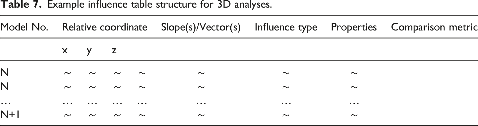
The comparison of these globally defined influences is achieved through comparing the relevant variables assigned to each influence type. Figure 11 shows the values associated to each influence designation that will be stored in a table that is structured in the same way as Table 7. In every instance, the material properties or boundary types are also included.

Figure 11.

Variation of values stored by the algorithm enabling comparisons to be made between each identified influence.

Table 7.

Example influence table structure for 3D analyses.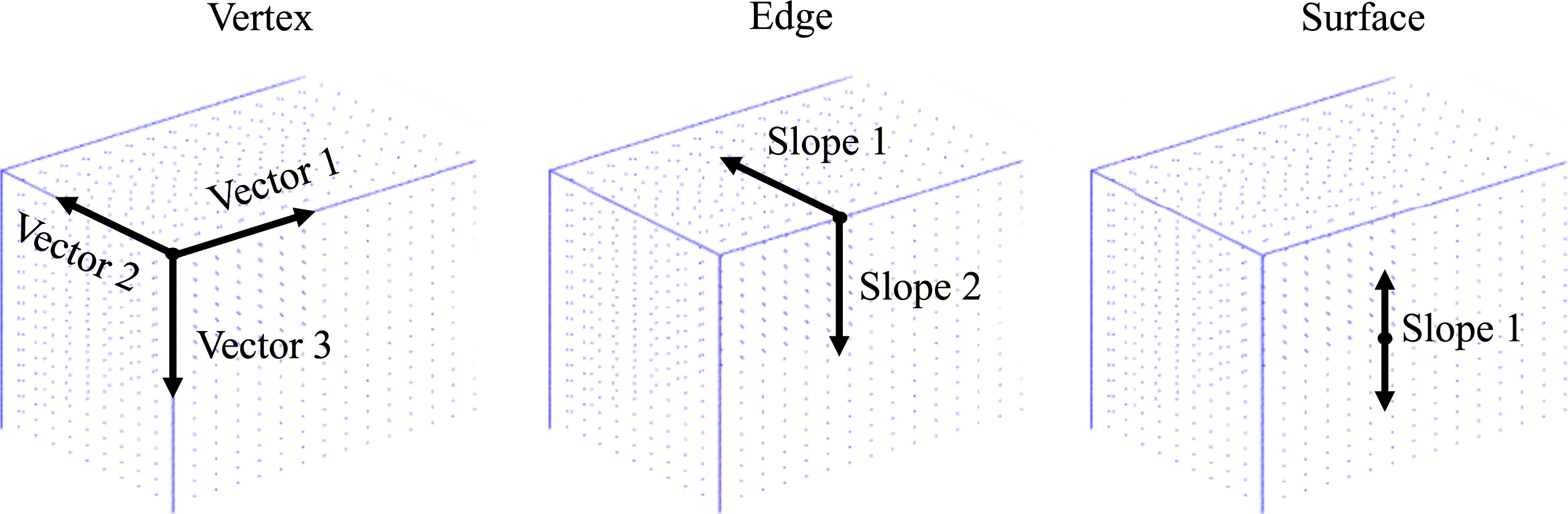

Model No.	Relative coordinate				Slope(s)/Vector(s)	Influence type	Properties
	x	y	z
N	∼	∼	∼	∼	∼	∼	∼
N	∼	∼	∼	∼	∼	∼	∼
…	…	…	…	…	…	…	…
N+1	∼	∼	∼	∼	∼	∼	∼

Blast wave path tracing

The comparison metric used to sort the influences according to the step where they are encountered in the numerical simulation was previously assigned to the direct distance between the charge and the relevant point to utilise the simplicity of the 2D geometry. However, this is not suitable for complex 3D models where the blast wave is expected to reflect off rigid surfaces and clear around object corners.

Ideally, the time of arrival of the blast wave would be calculated at each influence; however, there are currently no suitable rapid analysis methods for complex 3D geometries. The discrete series of nodes therefore acts as a connected graph upon which the blast wave can be tracked from the charge to each individual influence (or node). By considering the problem in this way, Dijkstra’s shortest path analysis is used to identify the shortest distance that the blast wave would have to travel to reach each relevant point of a given domain.

Figure 12 provides a visual representation of an influence mesh for a scaled city street curated by Brittle (2004). It also shows red lines that are formed considering the domain as a 3D graph, with shortest path analysis enabling the wave to be traced around the objects to a variety of points.

Figure 12.

Example shortest path analysis is used with a 3D connected graph to identify wave travel paths (red lines). Geometry shown is formulated in a study by Brittle (2004). Note that to improve image clarity no floor or boundaries has been defined for this arrangement and so the wave can be traced underneath the objects.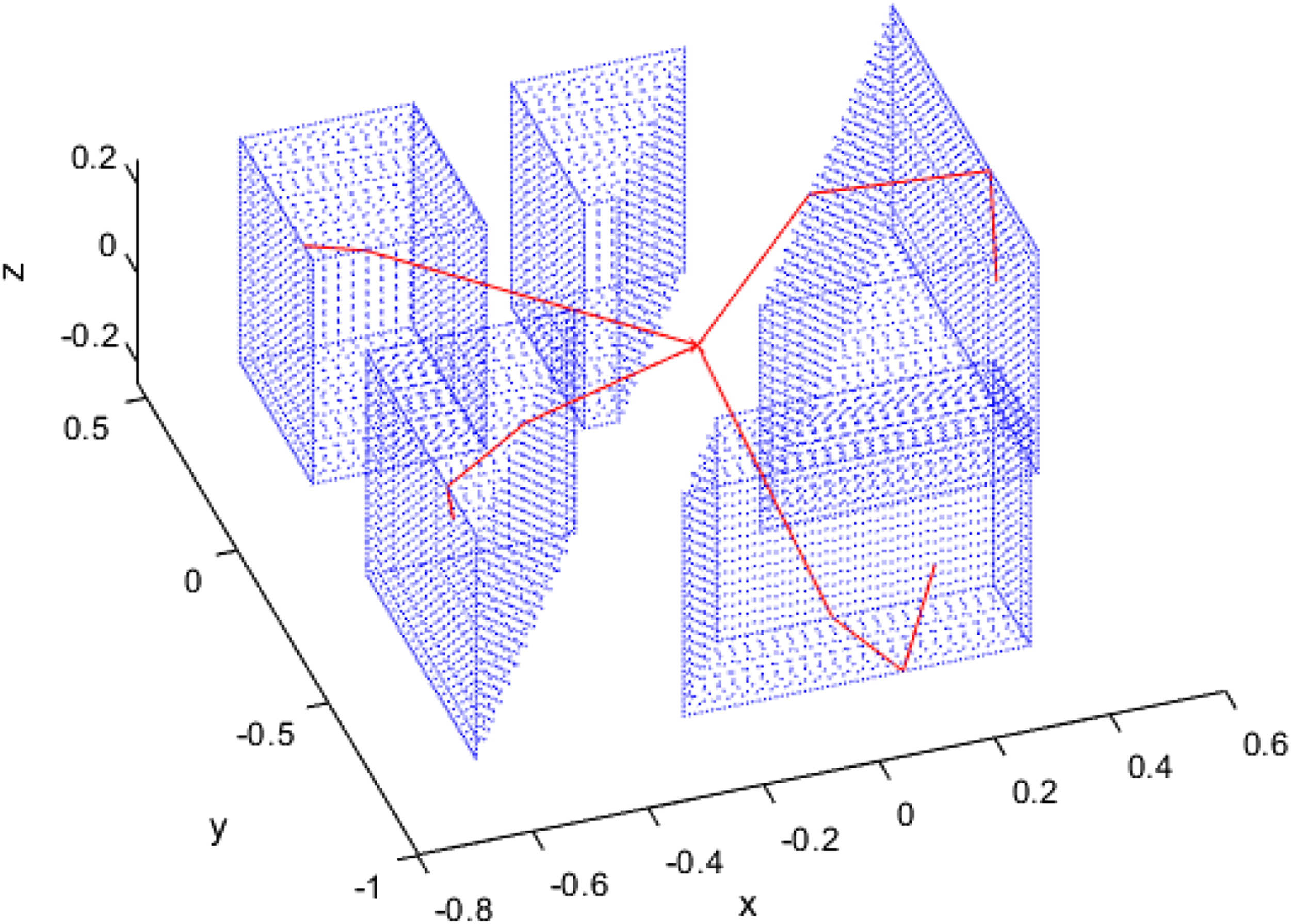

With these developments for influence generation and comparison, the algorithm can now be applied to 3D blast models using the same step-by-step procedure that was provided in The branching algorithm for blast analysis.

Example application in 3D

Problem scenario and model specification

Figure 13 provides a plan view of the 5 geometries that feature in a batch of 20, 3D models that aims to replicate a study where the effect of reducing the material use of geometry 1 is evaluated in terms of the overpressure that is recorded at key surrounding locations in the event of an accidental detonation. Each containment structure is 4 m tall, with base dimensions covering 18 x 5.5 m.

Figure 13.

Plan view of the five containment structures included in the example analysis.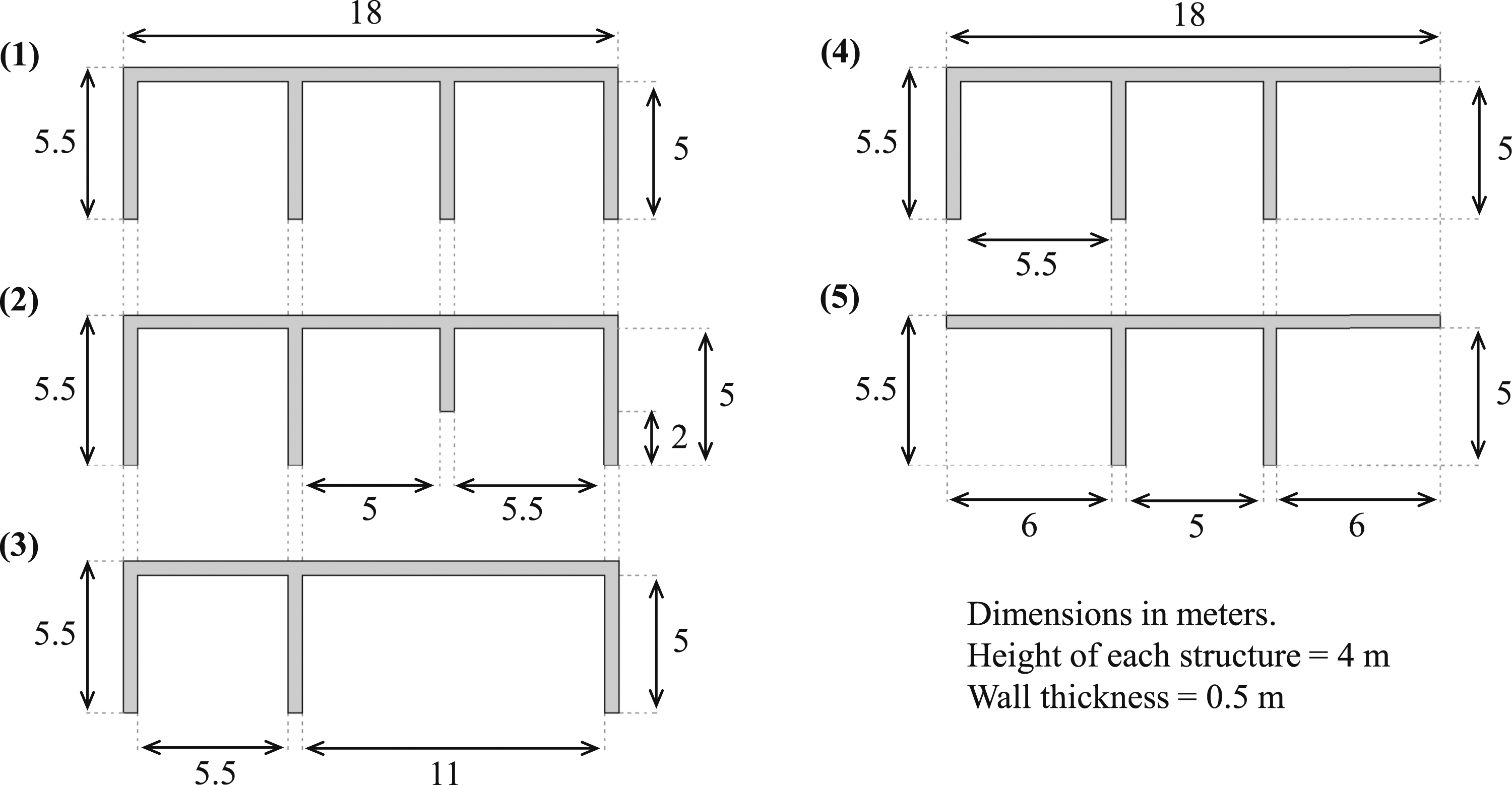

The locations of the gauges used to monitor the pressure variations are presented in Figure 14 alongside the four charge locations that are used independently with each geometry. Furthermore, the simulation domain that was adopted for use in the chosen computational fluid dynamics (CFD) solver, Viper::Blast (Stirling, 2021), is also provided. The floor is defined as the only reflecting surface with all others being able to transmit the blast wave outside of the domain.

Figure 14.

Plan view of the modelling domain, showing the origin point of the containment structures in Viper::Blast, four potential charge locations and five gauges used to record pressure-time profiles.

In each case, the Viper::Blast models are simulated using an ideal gas calculation with a 5kg, TNT, spherical charge positioned 1.5 m above the ground and a termination time of 55 ms. Ambient pressure and temperature are 101,325 Pa and 288 K, respectively. Simulations including the initial detonation utilised 1D to 3D mapping that takes place one cell before the wave reaches a rigid surface.

Unlike the previous example where LS-DYNA required validation for use in blast analyses, here the purpose written solver Viper::Blast does not require explicit validation. This is firstly because the results obtained from the analysis are not used in forming the conclusions of this article, with the focus instead being placed on the ability of the proposed method to save computation time. It is however important for the obtained results to be representative of the explosive scenario and since Viper::Blast is a tool founded upon established work published by Rose (2001) and Wada and Liou (1997), it is chosen approach for various studies including an air blast variability analysis conducted by Marks et al. (2021) and the evaluation of multiple simultaneously detonated charges by Zaghloul et al. (2021). This gives confidence that the observed parameters will be characteristic of an explosive test and therefore with progressive simulation time steps that represent typical blast analyses.

For all models, the element size of the 1D stage is specified as 0.002 m to provide ∼45 elements across the charge radius for the simulation of the initial detonation. As before, this surpasses the general requirement for around 10 elements to be used to ensure that the initial energy of the detonation process is preserved (Schwer and Rigby, 2018). This element size is increased to 0.04 m for the 3D stage.

A visual representation of all 20 models, including their numbers and charge locations is given in Figure 15.

Figure 15.

All 20 models included in the simulation batch. Each containment structure is modelled with each possible charge location.

Algorithm output

To identify the steps where informed data mappings can take place between the 20 models included in the given batch, the 3D geometries, boundaries and ambient conditions must be provided to the branching algorithm. In this example, the ambient conditions do not change in each domain and so the models are assigned to four trees, each corresponding to a charge location.

Figure 16 displays how the trees have been ordered, with red lines on each model showing the path of the wave from the charge to the uniquely identified deviation points. For lines that track through the containment walls, the wave is progressing up and over the 4 m structure. Domains including no red line are the trunk models of each group.

Figure 16.

Generated deviation trees and visual representations of the deviation points for each model. Red lines show the blast wave travel path to the first influence that results in a parameter field that is no longer identical to the parent model.

It should be noted that it is the final deviations being shown for each model in each tree. For example, reviewing the output for the first tree, model 5 deviates from the trunk model as the blast wave reaches the right hand wall of the central bay. No other model shows this to be a deviation point, however every other model also deviates from the trunk model at this step. Model 5 is therefore a sub-trunk model that was defined to enable greater computational savings. It is also only the final deviation point that is relevant for the initialisation of each domain in the batch, since the mapping order given by the deviation trees will be followed when transferring data between domains.

Simulation times

The overall computational saving is given by Table 8 where it is shown that full simulations of all 20 models requires 20,086 s when using an Intel i5-8265u processor, 8 GB of RAM and a Nvidia GTX 1650 dedicated graphics card. Utilising the branching algorithm and informed data mapping reduces this requirement to 16,228 s, providing a computation time saving of around 20%.

Table 8.

Comparison of model computation times.

Model No.	1	2	3	4	5	Tree 1
Without branching (s)	1039	1011	992	1030	1030	5102
With branching (s)	595	977	992	594	1001	4159
Saving (s)	444	34	0	436	29	943
Saving (%)	42.7	3.4	0	42.3	2.8	18.5
Model No.	6	7	8	9	10	Tree 2
Without branching (s)	1015	1009	1015	1013	986	5038
With branching (s)	351	599	971	603	986	3510
Saving (s)	664	410	44	410	0	1528
Saving (%)	65.4	40.6	4.3	40.5	0	30.3
Model No.	11	12	13	14	15	Tree 3
Without branching (s)	1013	1014	994	993	987	5001
With branching (s)	974	968	954	334	987	4217
Saving (s)	39	46	40	659	0	784
Saving (%)	3.8	4.5	4.0	66.4	0	15.7
Model No.	16	17	18	19	20	Tree 4
Without branching (s)	987	990	992	990	986	4945
With branching (s)	634	843	992	630	930	4029
Saving (s)	353	147	0	360	56	916
Saving (%)	35.8	14.8	0	36.4	5.7	18.5
Algorithm computation time:				313 s
Standard method computation time:				20086 s
Branched method computation time (inc. algorithm):				16228 s
Total saving (inc. algorithm):				19.2%
Branched method computation time (exc. algorithm):				15915 s
Total saving (exc. algorithm):				20.8%

For this complex scenario, a saving of around 20% means that an additional geometry could be assessed with all four charge locations at no extra cost when compared to the standard birth to termination simulation approach. Accordingly, an additional geometry could be explored that may benefit from the knowledge gained from the first batch at no additional computational cost.

When discussing the reported time saving, it is also important to consider how the individual computation requirements for each model are variable depending on the termination time and mesh density used in the numerical calculation. If these models were to have used higher resolution of elements, the relative cost of the algorithm would be reduced. This ultimately drives the total percentage saving to be closer to when the algorithm cost is ignored, in this case, moving 19.2% closer to 20.8%.

Furthermore, this sample study only contains 20 models. If instead, it featured upwards of 100 different arrangements with various combinations of geometry and charge size, it would be possible for a greater amount of saving to be observed with each model having a higher chance of sharing certain simulation steps with another in the batch.

Similarly, the solver Viper::Blast utilises Nvidia GPU processing in addition to various optimisation methods that significantly reduce the time required to analyse any given model when compared to alternatives exclusively featuring CPU processing power. Viper::Blast is therefore already likely to be a less time consuming approach to conducting batch analyses and so the savings noted here are expected to be far greater if less optimised solvers were to be used instead.

Regarding the implementation of the branching algorithm and data mapping, the algorithm could have used all models in one tree rather than splitting them into four separate trees. This would have increased the number of simulation steps being removed as the initial detonation of the charge, that was common to all models, would only need to be simulated once whereas here it was done four times. However, the sorting process used by the algorithm runs more efficiently with smaller trees because fewer model to model comparisons are required when defining the trunk model. Ultimately, this improved algorithm efficiency outweighs the potential saving of modelling the detonation once because the 1D solution used for this stage is already rapid in its execution.

Mapping results

As with the previous application, Figure 17 shows how the branched output for gauge 2 in model 9 is indistinguishable to the output from the same gauge when simulating the entire model without informed data mapping. The reduction in simulation time from 1013 s to 603 s for this model is therefore not affected by a reduction in the simulation accuracy.

Figure 17.

Pressure-time history recorded by gauge 2 when simulating model 9 entirely in its own domain (left) compared to when informed data mapping is used (right). Each line type shows which domain the data was record in.

Whilst it was not the aim of this paper to draw conclusions about the containment structures considering the magnitudes of the simulated results, with the focus instead being placed on proving the computation time saving potential of the branching algorithm, it is important to appreciate the scenario where the batch analysis approach is useful. Table 9 therefore provides the peak overpressure at each gauge for each containment structure (shown in Figure 13) considering all four potential charge locations. An assessment of these readings clearly shows how the variation between is small for gauges 2, 3 and 4. However, gauges 1 and 5 highlight how structures 4 and 5 may result in an unacceptable risk of increased overpressure either side of the containment model. Containment 3 appears to present the best compromise between peak values and material use, however no human vulnerability thresholds or fatality assessments, such as the ones featured in studies by Alterman et al. (2019) and Marks et al. (2021), have been consulted or conducted in making this judgement. Including such analyses would be required in the next phase of this analysis so that the data from all 20 models is utilised to make more informed risk based decisions or in designing a new alternative structural arrangement that benefits from these observations.

Table 9.

Comparison of the peak overpressure recorded at each gauge for each containment structure considering all charge locations.

Containment Structure	Peak Overpressure (kPa) at gauge number
	1	2	3	4	5
1	18.53	8.22	11.13	8.22	18.19
2	18.53	8.22	9.91	8.22	18.19
3	18.53	8.22	8.51	8.22	18.19
4	18.53	8.22	11.13	8.22	82.58
5	79.16	8.22	11.13	8.22	82.58

Conclusion

This paper has proposed and applied a new branching algorithm that can be used when modelling a range of similar numerical models with differing input parameters. The algorithm removes the need to simulate the steps of a simulation more than once if they occur within multiple models by identifying the similarities between the inputs and the newly defined ‘influences’.

It is shown that by using the developed approach for a simple blast analysis featuring 9 models, approximately 50% of the required computation time can be saved when compared to simulating each model independently. Similarly, when developing the influence definitions and applying the proposed method to a complex set of 20, 3D containment structures, the computation time can be reduced by approximately 20%.

A key advantage of utilising this method is therefore that it provides the researcher with the ability to conduct a more robust analysis of various problems with the same computation expense. Thus benefiting the analysis of probabilistic frameworks, or development of machine learning training datasets to ultimately promote more effective design optimisation and exploration. The ability to remap data from one domain to another relative to the centre of an explosion lends itself well to transferring data at time steps where a deviation in the outputs will occur, however, the magnitude of the improvement to the required computation time will vary depending on the application and complexity of the batch of models being simulated.

The key contribution of this work is that it provides a robust, reliable and repeatable method for formalising efficient remapping of numerical modelling, by identifying a main ‘trunk’ model and sorting each subsequent model according to when its results are expected to deviate from that model. Whilst this article focusses on blast analyses, future applications could look to tailor and develop the algorithm for different numerical problems, where batches of models are equally as important for understanding the processes being models. This includes vehicle design and safety assessments (e.g. Lu et al., 2020; Wu et al., 2020), search and rescue tools (e.g. Coppini et al., 2016), pressurised water pipe failure (e.g. Barr et al., 2020) and structural topology optimisation.

Future developments focussed on the method’s usability for blast analyses includes automating the execution stage of the proposed method. At present, the order of effective simulation is automatically generated by the algorithm using the batch inputs, but manual intervention is required when using the chosen numerical solver to export the parameter field as a change in ambient conditions is observed at each deviation condition and when initialising each of the models with the relevant data map that has been produced. Nevertheless, the recorded simulation times presented in this study remain consistent with if the full process were to be carried out with no manual intervention. Thus proving that a solver that is able to monitor deviation points, export parameter fields and initialise models using this data automatically can be used in conjunction with the branching algorithm to reduce batch computation times.

Lastly, as the branching algorithm presented herein operates as a forward model (causalities → effects), in future work we aim to investigate the feasibility of inverting the framework (effects → causalities). Pragmatically, such an inverse approach may afford users the ability to directly approximate realisations, such as charge size, location and type, directly from spatial-temporal measurements, having application in post-blast prognosis and site investigation. From a technical standpoint, an inverse truncated model may offer numerical benefits, for example, conditional well-posedness, reduced sensitivity to measurement noise/error and reduced computational demand.

Footnotes

Acknowledgement

Adam A Dennis gratefully acknowledges the financial support from the Engineering and Physical Sciences Research Council (EPSRC) Doctoral Training Partnership.

Declaration of conflicting interests

The author(s) declared no potential conflicts of interest with respect to the research, authorship, and/or publication of this article.

Funding

The authors disclosed receipt of the following financial support for the research, authorship, and/or publication of this article: This study was supported by grants from Engineering and Physical Sciences Research Council (EPSRC) Doctoral Training Partnership.

ORCID iDs

Adam A Dennis

Chris G Stirling

Samuel E Rigby

Appendix

References

Alterman

Stewart

Netherton

(2019) Probabilistic assessment of airblast variability and fatality risk estimation for explosive blasts in confined building spaces. International Journal of Protective Structures 10(3): 306–329.

Aquelet

Souli

(2008) 2D to 3D ALE mapping. In: 10th International LS-DYNA Users Conference, Dearborn, MI, USA, 8–10 June 2008, pp. 23–34.

Barr

Rigby

Collins

, et al. (2020) Predicting crater formation from failure of pressurized water mains through analogy with buried explosive events. Journal of Pipeline Systems Engineering and Practice 11: 04020013.

Belhamadia

Fortin

Bourgault

(2014) On the performance of anisotropic mesh adaptation for scroll wave turbulence dynamics in reaction-diffusion systems. Journal of Computational and Applied Mathematics 271: 233–246.

Berger

Colella

(1989) Local adaptive mesh refinement for shock hydrodynamics. Journal of Computational Physics 82(1): 64–84.

Bortolan Neto

Saleh

Pickerd

, et al. (2020) Rapid mechanical evaluation of quadrangular steel plates subjected to localised blast loadings. International Journal of Impact Engineering 137: 103461.

Brittle

(2004) Blast Propagation in a Geometrically Complex Environment, PhD thesis. Cranfield University.

Bruneau

Khadra

(2016) Highly parallel computing of a multigrid solver for 3D Navier–Stokes equations. Journal of Computational Science 17: 35–46.

Coppini

Jansen

Turrisi

, et al. (2016) A new search-and-rescue service in the Mediterranean Sea: a demonstration of the operational capability and an evaluation of its performance using real case scenarios. Natural Hazards and Earth System Sciences 16(12): 2713–2727.

10.

Cranz

(1926) Lehr der Ballistik. Berlin, Germany: Verlag von Julius Springer.

11.

Dennis

Pannell

Smyl

, et al. (2021) Prediction of blast loading in an internal environment using artificial neural networks. International Journal of Protective Structures 12(3): 287–314.

12.

Hopkinson

(1915) Board Minutes, 13565. British Ordnance.

13.

Lapoujade

Van Dorsselaer

Kevorkian

, et al. (2010) A study of mapping technique for air blast modeling. In: 11th International LS-DYNA users Conference, Detroit, Blast/Impact, pp. 23–32.

14.

Shen

Wang

, et al. (2020) Studying on the design and simulation of collision protection system between vehicle and pedestrian. International Journal of Distributed Sensor Networks 16(1): 155014771990010.

15.

Marks

Stewart

Netherton

, et al. (2021) Airblast variability and fatality risks from a VBIED in a complex urban environment. Reliability Engineering and System Safety 209: 107459.

16.

Murmu

Maheshwari

Verma

(2018) Empirical and probabilistic analysis of blast-induced ground vibrations. International Journal of Rock Mechanics and Mining Sciences 103: 267–274.

17.

Park

Kwon

(2005) A parallel unstructured dynamic mesh adaptation algorithm for 3-D unsteady flows. International Journal for Numerical Methods in Fluids 48(6): 671–690.

18.

Peery

Carroll

(2000) Multi-material ALE methods in unstructured grids. Computer Methods in Applied Mechanics and Engineering 187(3–4): 591–619.

19.

Zhi

Fan

, et al. (2020) Probabilistic blast load model for domes under external surface burst explosions. Structural Safety 87: 102004.

20.

Rebelo

Cismasiu

(2021) Robustness assessment of a deterministically designed sacrificial cladding for structural protection. Engineering Structures 240: 112279.

21.

Rigby

Akintaro

Fuller

, et al. (2019) Predicting the response of plates subjected to near-field explosions using an energy equivalent impulse. International Journal of Impact Engineering 128: 24–36.

22.

Rigby

Knighton

Clarke

, et al. (2020) Reflected near-field blast pressure measurements using high speed video. Experimental Mechanics 60(7): 875–888.

23.

Rigby

Fuller

Tyas

(2018) Validation of near-field blast loading in LS-DYNA. 5th International Conference on Protective Structures 1: 1–8.

24.

Rose

(2001) An Approach to the Evaluation of Blast Loads on Finites and Semi-infinite Structures, Phd thesis. Cranfield University.

25.

Schwer

Rigby

(2018) Secondary and height of burst shock reflections : application of afterburning. In: Proceedings of the 25th Military Aspects of Blast and Shock (MABS25)’, Military Aspects of Blast and Shock, Netherlands. The Hauge.

26.

Seisson

Lacaze

Rouquand

(2020) Uncertainty estimation of external blast effects using the monte-carlo method. WIT Transactions on the Built Environment 198: 81–92.

27.

Stewart

Netherton

(2015) Reliability-based design load factors for explosive blast loading. Journal of Performance of Constructed Facilities 29(5): 1–8.

28.

Stewart

Netherton

Rosowsky

(2006) Terrorism risks and blast damage to built infrastructure. Natural Hazards Review 7(3): 114–122.

29.

Stirling

(2021) Viper::Blast. Edinburgh, Scotland: Stirling Simulation Services Limited.

30.

Wada

Liou

(1997) An accurate and robust flux splitting scheme for shock and contact discontinuities. SIAM Journal of Scientific Computing 18(3): 633–657.

31.

Tseng

(2005) Parallel DSMC method using dynamic domain decomposition. International Journal for Numerical Methods in Engineering 63(1): 37–76.

32.

Jin

(2020) Dynamic responses and reliability analysis of bridge double-column under vehicle collision. Engineering Structures 221(July): 111035.

33.

Zaghloul

Remennikov

(2021) Enhancement of blast wave parameters due to shock focusing from multiple simultaneously detonated charges. International Journal of Protective Structures 12(4): 541–576.

Model No.	Relative coordinate				Slope(s)/Vector(s)	Influence type	Properties
	x	y	z
N	∼	∼	∼	∼	∼	∼	∼
N	∼	∼	∼	∼	∼	∼	∼
…	…	…	…	…	…	…	…
N+1	∼	∼	∼	∼	∼	∼	∼

Model No.	Relative coordinate				Slope(s)/Vector(s)	Influence type	Properties
	x	y	z
N	∼	∼	∼	∼	∼	∼	∼
N	∼	∼	∼	∼	∼	∼	∼
…	…	…	…	…	…	…	…
N+1	∼	∼	∼	∼	∼	∼	∼

A branching algorithm to reduce computational time of batch models: Application for blast analyses

Abstract

Keywords

Introduction

The branching algorithm

Principles and terminology

The branching algorithm for blast analysis

Example application in 2D

Problem scenario

Validation of LS-DYNA for blast analysis

Model specification

Algorithm walk-through and output

Simulation times

Mapping results

Developments for 3D analyses

Domain discretisation and influence comparison

Blast wave path tracing

Example application in 3D

Problem scenario and model specification

Algorithm output

Simulation times

Mapping results

Conclusion

Footnotes

Acknowledgement

Declaration of conflicting interests

Funding

ORCID iDs

Appendix

References

Model No.	Relative coordinate				Slope(s)/Vector(s)	Influence type	Properties
	x	y	z
N	∼	∼	∼	∼	∼	∼	∼
N	∼	∼	∼	∼	∼	∼	∼
…	…	…	…	…	…	…	…
N+1	∼	∼	∼	∼	∼	∼	∼