Sage Journals: Discover world-class research

Abstract

The ability to accurately determine blast loading parameters will enable more fundamental studies on the sources of blast parameter variability and their influence on the magnitude and form of the loading itself. This will ultimately lead to a better fundamental understanding of blast wave behaviour, and will result in more efficient and effective protective systems and enhanced resilience of critical infrastructure. This article presents a study on time of arrival as a diagnostic for far-field high explosive blasts, and makes use of the results from a large number of historic tests and newly performed experiments where the propagating shock front was filmed using a high-speed video (HSV) camera. A new method for optical shock tracking of far-field blast tests is developed and validated, and full-field arrival time results are compared against those determined from the historic data recorded using traditional pressure gauges. Arrival time variability is shown to be considerably lower than peak pressure and peak specific impulse, and is shown to decrease exponentially with increasing scaled distance. Further, the method presented in this article using HSV cameras to determine arrival time yields further reductions in variability. Finally, it is demonstrated that the method can be used to accurately determine far-field TNT equivalence of high explosives.

Keywords

Blast time of arrival high speed video image tracking variability

Introduction

Designing for resilience against the damaging effects of explosions is becoming an increasingly important structural design. Here, accurate quantification of the magnitudes of loading imparted to a structure is of paramount importance, and related to this is the ability to characterise input parameters and physical mechanisms which govern the development of this loading. Variations in blast load parameters (termed blast parameter variability) from nominally identical experimental testing are frequently observed, yet their origins and prominence have yet to be fully studied. Accurate establishment of blast parameter variability, across a wide range of distances from the explosive origin, has implications for probabilistic-based design and the development of fast-running predictive models. It is well documented that the effects of a given explosive event vary when repeated, which poses issues for the accuracy and efficiency of blast resilient designs. Establishing blast parameter variability ranges, with respect to scaled distance, provides the basis for probabilistic-based approaches which could be integrated into fast-running predictive models. Through inclusion of the variability each parameter exhibits across a full-field of distances, more effective explosive-resilient structural designs can be developed.

Blast wave time of arrival, t_a, has been shown to be the most deterministic and repeatable blast parameter (Rigby, 2021). Since peak incident and reflected pressures can be inferred from t_a, using Rankine–Hugoniot jump conditions (Ohashi et al., 2001), it can be said that definitive knowledge of how t_a, and its associated variability, changes with scaled distance can lead to a more fundamental understanding of the sources of variability in blast pressure measurements.

A limitation of current pressure gauge-based experimental measurements is that t_a can only be recorded at discrete distances away from the explosive centre, and, there are limitations to how close gauges can be located. Therefore, in order to determine blast time of arrival experimentally, a large number of tests or a high instrumentation demand is required. Alternatively, optical techniques (Anderson et al., 2016; Hargather, 2013) can be used to track the position of the shock front at high resolution and frame rate. This article presents a method of recording arrival time data across a much wider field of distances for a single given trial and uses this data to quantify experimentally recorded variability, as a function of scaled distance. The recorded videos were processed with an in-house tracking and interpolation algorithm with the results being used to make comparisons to the typical variability in pressure and arrival time measurements resulting from autonomous curve-fitting gauge analysis implemented on historical data.

The paper is structured in the following manner. First, a comprehensive literature review outlines the state-of-the-art in both the assessment of blast parameter variability, and the use of shock wave arrival time as an investigative tool. Then, an overview of the experimental set-up is provided, which has been used for historic tests and the newly performed tests described in this article. Subsequently, we detail two different methods for data analysis: a method for automated analysis of pressure gauge data (to reduce subjectivity and variabilities in data processing), and; a method to determine shock front arrival times from processing high-speed video (HSV) footage using edge detection and image subtraction. Finally, we discuss the variabilities associated with both approaches, and conclude by providing a practical example of determining explosive yield from arrival time data.

Literature review

Variability of blast wave parameters

There has been significant research undertaken into expanding the fundamental understanding of explosive events within the last century, alongside characterising resulting blast wave features through experimental analysis (Kennedy, 1946). Both Baker (1973) and Esparza (1986) provide summaries of contemporary and historical experimental quantification of blast parameters.

The Kingery and Bulmash (1984) predictive method, hereafter shortened to KB, was derived from a large database of existing experimental trials and can be used to estimate the loading conditions associated with a given spherical, or hemispherical, charge at a set distance away from a target. Considerable amounts of research has compared experimental results to KB predictions, which in turn has validated the standard for predictions of positive phase blast parameters in far-field scenarios (Bogosian et al., 2002). As a result, the KB method is widely recognised as an effective fast-running predictive tool for positive phase blast parameters, and has been implemented into the UFC 3-340-02 design manual (US Department of Defence, 2008), the predictive computer code Conwep (Hyde, 1991), and commercial finite element code LS-DYNA (Randers-Pehrsons and Bannister, 1997), among others.

Despite a general confidence in the KB method, recent articles have demonstrated varying levels of agreement with KB predictions, mainly attributed to large test-to-test variations in experimental measurements of blast load parameters and difficulties in establishing a reliable experimental benchmark. Bogosian et al. (2002) utilised an extensive experimental database to compare these with the KB predictions, with the analysis suggesting that that reflected peak pressure and specific impulse have shown to exhibit variations of between 70–150% and 50–130%, respectively, from nominally identical tests when compared directly to the KB method. Tang et al. (2017) found that incident and reflected pressures exhibit different levels of variability to one-another but that inconsistencies in pressure measurements occur at all stand-off distances. Netherton and Stewart (2010) made attempts at statistically quantifying variability associated with blast events which resulted in conservative predictions when compared to experimental results. This highlights the need for a more precise quantification of blast parameter variability with respect to scaled distance which could then be integrated with KB, or alternative, predictive methods to achieve greater confidence in prescribed blast design criteria.

It has been hypothesised that the levels of variability are inherent features of all explosive events, and the precise quantification of blast parameters will always be difficult to establish. Smith et al. (1999) suggested that it is essential to conduct repeat tests to have confidence in the variability of measurements. However, both Rickman and Murrell (2007) and Tyas et al. (2011) observed very low levels of uncertainty in recorded blast parameters and presented high levels of test-to-test repeatability alongside agreement to the KB predictions.

Rigby and Sielicki (2014) compared the results from explosive trials with numerical analyses and concluded that in the far-field (6.0–14.9 m/kg ^1/3), PE4 has a consistent TNT equivalence value of 1.20. This suggests that any features driving variations in blast parameters do not persist into the far-field, and therefore we should expect blast parameter variability to decrease as the situation approaches the far-fields. Rigby et al. (2014a) quantified the variability associated with each blast parameter from highly controlled experimental recordings when compared to KB predictions, and grouped results from nominally identical tests. The presented results and the KB predictions held high levels of agreement, exhibiting variability of between ±6–8% for pressure and specific impulse parameters, ±2.5% for shock front arrival time and around ±9% for positive phase duration. The findings suggest that blast load variability can be considerably reduced in well-controlled experimental trials but not eliminated, emphasising the requirement of variability quantification and its inclusion into predictive methods for more accurate prescribed loading conditions.

There is further evidence to suggest that key loading parameter variability reduces with respect to an increase in scaled distance. Bogosian et al. (2014) performed air-blast tests using 11 cylindrical charges and recorded pressure-time histories at five different gauge locations, comparing the findings to historical incident data (Ohrt et al., 2014) between 0.6 and 3.4 m/kg^1/3 scaled distance. The peak pressures and positive phase specific impulses were evaluated statistically to obtain the levels of blast parameter variability. The findings were as follows: impulse measurements were inherently more reliable than those for peak pressure; closely spaced gauge recordings from a single explosive event, with nominally scaled distances, showed variability in the measurements; and, blast parameter variability tended to decrease as scaled distance increased. The overall conclusion when comparing variability ranges between specific scaled distances was that something other than chaotic variability was introducing rises in experimental uncertainty. This is believed to support separate observations of significant undulations in the expanding shock front as a result of instability formation, although the full extent of this is yet to be fully quantified.

Tyas (2019) hypothesised the existence of three distinct ranges of scaled distances where shock front behaviour differs: at the extreme near-field (≤0.5 m/kg^1/3) and far-field scaled distances (≥2 m/kg^1/3), the data recorded by pressure gauge tests is highly repeatable and consistent, but at the intermediate distances (0.5–2 m/kg^1/3), higher variability is experienced in the recorded blast parameters. Rae and McAfee (2018) experimentally tested ground-detonated large hemispheres of C-4 to measure blast parameters at scaled distances between 0.5 and 1.8 m/kg^1/3 and noted the presence of three similar regions. Rigby et al. (2020a) used image tracking methods for near-field blast pressure predictions which resulted in similar findings. It was hypothesised that the results displayed two distinct stages of emergent instabilities in the fireball/shock-air interface. In the early stages after detonation, prior to or shortly after the emergence of small turbulence-based instabilities, the fireball/air interface was seen to expand with effectively deterministic velocity. Beyond 10 charge radii, the instabilities experienced large growths giving rise to more chaotic behaviour of the interface and thus an increasing uncertainty in surface velocity. These studies all suggest that blast parameter variability is associated with the development and curtailment of RT (Rayleigh, 1882; Taylor, 1950) and MR (Meshkov, 1969; Richtmyer, 1960) surface instabilities in the expanding fireball and shock front. RT instabilities occur when pressure and density gradients are in opposite directions, that is, when detonation products expand and compress a surrounding medium until the medium’s pressure exceeds that in the fireball but the air density is significantly lower. RM surface instabilities are the result of shock wave propagation through inhomogeneous media (formed a result of RT instabilities). Schoutens (1979) and Tyas et al. (2016) both observed significant localised changes in blast parameter quantification on reflected surfaces as a direct result of instability formation. Whilst it has been observed that these instabilities begin to diminish for far-field scenarios, accurate determination of their formation, with respect to scaled distance, is yet to be fully established. Despite the aforementioned work on blast parameter variability, there remains no widely agreed method for quantifying typical variations in a statistically robust sense for a given experimental trial. As a result, it is difficult to prescribe accurate loading condition ranges a structure may experience as a result of an explosive event.

Shock wave arrival time

Blast pressure signals exhibit a level of sensor ringing due to mounting conditions and inertial response of the gauge, as well as some background levels of electrical noise, which makes interpretation of some key metrics, such as peak pressure, positive phase duration and thus peak specific impulse, difficult. During experimental trials, the arrival time of a shock front, t_a, is recorded as a near-instantaneous rise above atmospheric conditions, making more precise determination possible (Rigby et al., 2014a). Whilst the quantification of peak pressure, positive phase duration and peak specific impulse are requirements for assessing structural response to explosive effects, shock wave time of arrival is able to provide fundamental understanding into the form and magnitude of a blast wave (Rigby, 2021).

Traditional blast measurement techniques using pressure gauges (Rigby et al., 2014a), impulse plugs (Nansteel et al., 2013) and Hopkinson pressure bars (Clarke et al., 2014), record a single t_a per measurement location, hence full-field arrival time quantification is not feasible using these methods without an extensive testing plan or high instrumentation/data acquisition demand. Alternatively, optical recording of propagating shock waves using HSV cameras has the potential to provide full-field shock wave radius measurements and hence determination of arrival time (and variations thereof) as a function of distance from the charge centre.

Extensive research has been undertaken in evaluating shock wave pressure using well know pressure-velocities relationships alongside HSV recordings. Dewey (1971) began to investigate t_a measurements and how they could be manipulated to determine physical properties of propagating blast waves, making comparisons between photographic and electronic recording methods.

More recent works by Hargather (2013) and Mizukaki et al. (2014) both used background oriented schlieren methods during large-scale explosion events to obtain shock wave propagation velocities in order to estimate incident pressures. Kucera et al. (2017) performed similar tests, recording propagating shock waves from smaller scale charges. The optically evaluated pressures from each of these studies demonstrated reasonable levels of agreement with gauge recordings between 0.8 and 5.2 m/kg^1/3. Pontalier et al. (2021) undertook a comprehensive optical analysis of shock wave propagation from metalized explosives across the intermediate scaled distance range (1.0–3.5 m/kg^1/3), measuring both fireball and fragment expansion rates. The results of which presented reasonably high variability of both arrival time and peak pressure when comparing nominally identical tests.

Further developments have been made into methods of optically inferring the specific impulse of an explosive event when cameras were used in conjunction with pressure gauges. Biss and McNesby (2014) developed a method which looked at optically obtained spatio-temporal pressure maps and integrated with respect to gauge recorded positive phased durations in the 100 kPa range. Anderson et al. (2016) developed a theoretical estimate for the blast decay coefficient of the modified Friedlander equation, which was used to predict the positive phase pressure-time profile. Whilst both methods present reasonable estimates for specific impulse calculation, a general under-prediction when compared to KB predictions was seen.

Following the large explosion at the Port of Beirut, Lebanon, in August 2020, a method of calculating explosive yield was presented based on the relationship between arrival time and stand-off, determined at various locations in the city using 16 smart device video recordings posted to social media after the explosion (Rigby et al., 2020b). The relatively high agreement between the processed results and KB predictions, despite relatively low precision and quality of the recordings, provides clear initiative to continue research using t_a through the use of HSV in well-controlled experimental trials.

Despite significant research interest in shock wave time of arrival, there is limited knowledge the variability of this parameter. Quantification of shock front arrival time variability with respect to scaled distance could provide a basis from which to develop a better understanding of RT and RM instability formation and dissipation. Further, an improved knowledge of statistical variations in shock wave arrival time would allow for the development of more comprehensive and accurate probabilistic blast load predictive methods.

Experimental setup

A total of 10 experiments were performed at the University of Sheffield (UoS) Blast and Impact Laboratory in Buxton, UK. Far-field arena-style tests were performed using 250 g hemispherical charges of PE4 at scaled distances of 3.0–12.0 m/kg^1/3.Of the 20 individual pressure recordings, 13 provided credible data and are reported on in this article. Additionally, a further 144 historic pressure gauge recordings are utilised as part of this work (Rigby et al., 2014b, 2015; Tyas et al., 2011), comprising data from hemispherical PE4 charges between 180 and 350 g at scaled distances of 1.9–15.0 m/kg^1/3. All tests were performed as part of a wider research project which aims to characterise how blast parameters vary both spatially and temporally across a comprehensive range of scaled distances. Data were recorded using piezo-resistive pressure gauges in the historic tests, and using a combination of piezo-resistive pressure gauges and HSV cameras in the new tests described in this article. Figure 1 shows the configuration of the far-field arena trials.

Figure 1.

General arrangement of the test pad at the University of Sheffield Blast and Impact Laboratory: Site photograph taken approximately from the location of the high-speed video camera.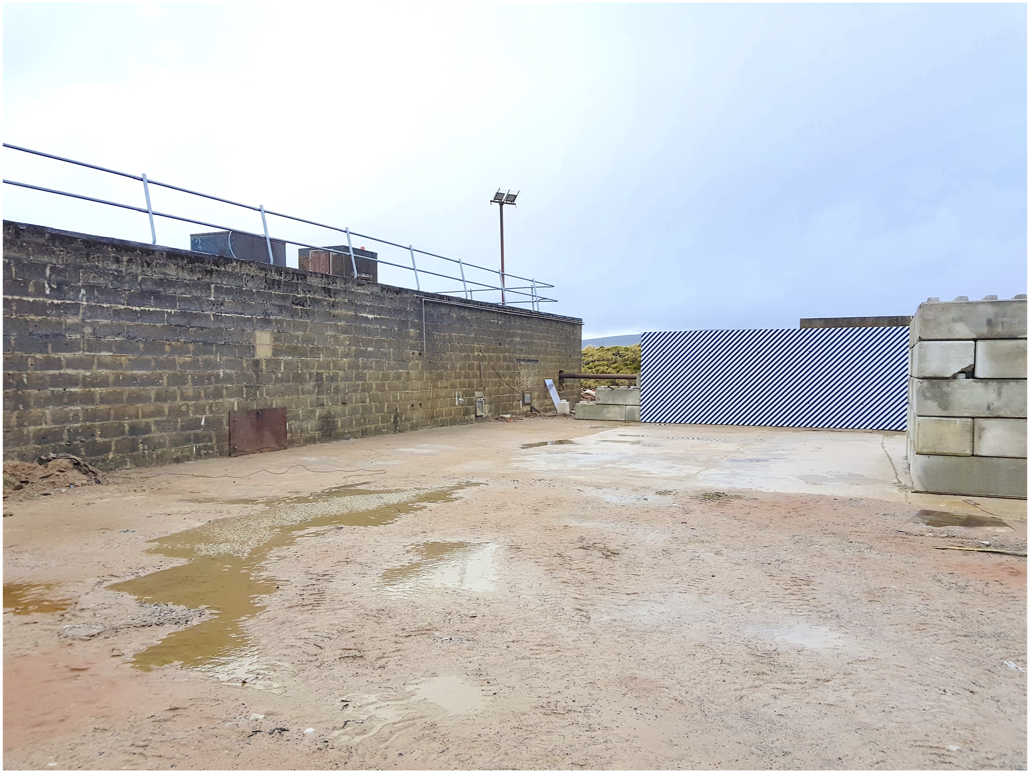

For each of the 10 newly performed trials, 250 g hemispherical PE4 explosive charges, formed using a 3D-printed mould, were detonated at varying stand-off distances, R_a and R_b in Figure 2, perpendicular to rigid reflective surfaces in the form of a reinforced concrete bunker and a blockwork wall, separated exactly 10.0 m apart. Kulite HKM-375 piezo-resistive pressure gauges threaded through, and made flush to the surface of a small steel plate (approximately 200 × 200 × 10 mm) fixed to these walls, were used to record the reflected pressure history in each test at each location. The charges were placed on another small steel plate prior to detonation, avoiding repeat extensive damage to the concrete testing pad between tests. The pressure was recorded using a 16-bit digital oscilloscope and TiePie software, with an average sampling rate of 195 kHz at 16-bit resolution. The recording was triggered automatically using TiePie’s ‘out window’ signal trigger on a bespoke break-wire signal, formed by a wire wrapped around the detonator. The ‘out window’ trigger initiated with a voltage drop outside the normal electrical noise experienced in the break-wire. This coincides with the detonation of the charge breaking the circuit.

Figure 2.

General arrangement of the test pad at the University of Sheffield Blast and Impact Laboratory: Schematic including HSV camera positioning.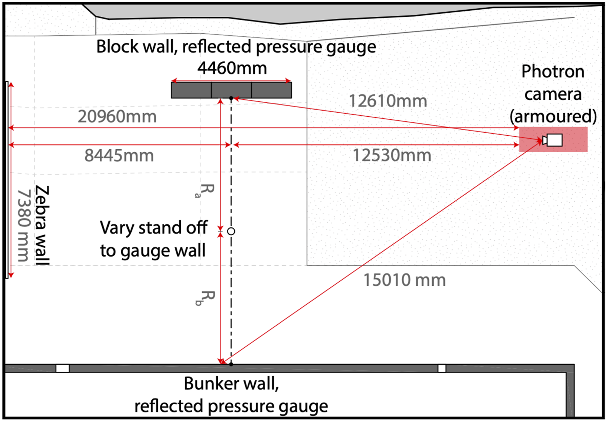

In the current tests, HSV recordings of the propagating shock front were taken in an attempt to quantify the variability of shock wave arrival time recordings. As seen in Figure 2, the explosive charges were situated between a Photron FASTCAM SA-Z HSV camera, fitted with a Tamron SP AF70 70–200 mm zoom (F2.8) lens, and a zebra board which ran perpendicular to the blockwork and bunker walls. The camera was positioned to record the shock wave as it propagated towards the blockwork wall and had the charge location out of the camera’s field of view to avoid excessive light from the fireball corrupting the contrast of the images. The camera was placed inside an armoured protective housing to avoid any fragment damage during testing.

A long-span zebra board served to provide a high contrast background such that distortions in light, caused by changes in refractive index of the propagating shock front, would feature as sharp dark bands in the HSV recordings. This allows the position of the shock front to be identified in each frame, and therefore enables wider-field arrival time measurements from a given trial (Igra and Seiler, 2016). The frame rates of the recordings and exposure time varied between 10,000–36,000/s and 9.4–26.2 μs due to varying weather/light conditions. Frame rates and exposure times were altered before to each test in order to maximise the contrast of the zebra board stripes, and the sharpness of the propagating shock front.

Pressure gauge analysis

Introduction

Raw pressure-time histories tend to exhibit large uncertainties in the opening few microseconds after the arrival of a shock, and throughout the whole trend, associated with sensor ringing and natural electrical noise, respectively (Rigby et al., 2014a). Precise determination of key blast wave parameters is therefore challenging and alluding to an emphasis on the importance of functional signal analytics for higher levels of precision (Bogosian et al., 2019).

Background electrical noise precludes accurate and automatic determination of the positive phase duration, t_d of a pressure signal, since a recorded signal may oscillate around the origin for a non-zero period of time. Further, it has previously been shown that the specific impulse of a pressure signal can vary significantly depending on which value of positive phase duration (i.e. the time at which a pressure value at or near ambient is recorded) is taken (Lyons, 2012). A solution is to fit a modified Friedlander curve (equation (1)) to the experimentally recorded data which results in blast parameters showing agreement to numerical models (Tang et al., 2018) and empirical predictive methods (Rigby et al., 2014a)

P (t) = P_{\max} (1 - \frac{t}{t_{d}}) e^{- b (t / t_{d})}

(1)

Omitting the initial 25% of the positive phase duration from the fit has been shown to substantially increase the reliability of such a fit by lessening the effect of sensor ringing. This served to consistently reduce the observed test-to-test variability and increasing the agreement between experimentally measured parameters and KB predictions (Rigby et al., 2014a).

This section will examine techniques for automatically fitting a modified Friedlander curve to recorded pressure signals, in order to determine how best to accurately and robustly quantify variability of the pressure signal without introducing user error. This will provide a more reliable benchmark such that variabilities associated with shock wave arrival time can be compared in a more robust sense later in this article. The automated method was initially validated using 65 of the 144 PE4 historic trials (Rigby et al., 2015), and was then used to process all 13 recordings from the current trials. In addition to providing an accurate and repeatable method for processing signals, a secondary aim was to assess the veracity of omitting the first 25% of the positive phase impulse when curve-fitting, and whether this could be applied as a general rule.

Determination of best-fitting procedures

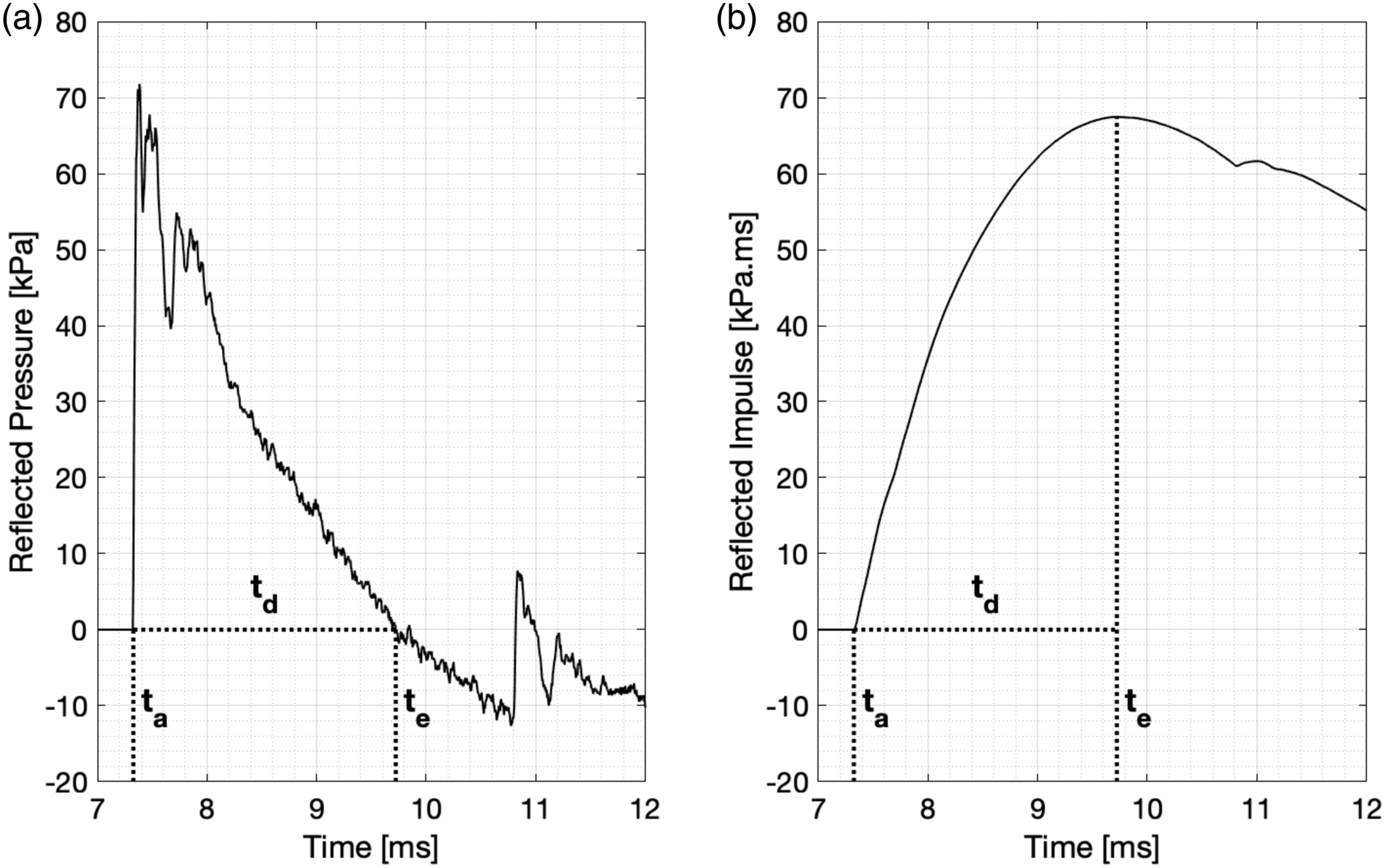
The general algorithm of the curve-fitting routine is as follows:

1. Determination of t _a: Typically recorded as a sharp, unambiguous rise to peak pressure, with a maximum rise time of only a few $(< 10)$ recorded samples(50 μ s). This can be seen in Figure 3(a) and is easily discernible in the raw data, that is, the main peak in the gradient of the pressure signal (Rigby and Gitterman, 2016).

Figure 3.

Example historic test results using a 250 g PE4 hemispherical charge at 4 m stand-off: (a) Raw pressure, and; (b) Raw specific impulse with respect to time for a single test, highlighting the assignment of shock wave arrival time, t_a, and positive phase duration, t_d.

2. Assignment of t _d: The electrical noise in the current set up was recorded and shown to be normally distributed around the true mean value meaning that when integrating pressure, with respect to time, the effect of electrical noise cancels out and has negligible effect on peak specific impulse. Therefore, the difference between the assigned t_a and the time at which the maximum specific impulse occurred would be assigned as the positive phase duration, t_d.

3. Incremental removal of start of positive phase: Inputting the time-based parameters and the raw pressure-time data into equation (1) provides a generalised curve with corresponding values for peak pressure and the decay coefficient, P_max and b, respectively. These parameters were fit to successively more curtailed pressure signals (in increments of a single percent, starting with the full signal), obtaining a spectrum of different peak pressures, specific impulses and decay coefficients from the results of a single test.

4. Determination of optimal removal ratio: Peak pressure and peak specific impulse values were seen to form a ‘fan’ around a central representative value. This was caused by regular features in the data induced by sensor ringing and inherent electrical noise. The mean values of the collated results for both peak pressure and specific impulse were calculated and the curve fits which satisfied both mean values within a ±5% region were defined as the ‘optimal model fits’ to the raw data. The mean of these parameters were then evaluated, giving the automatically generated peak pressure and peak specific impulse from that test. The decay coefficient was determined from iteration of the integral equation (1), after Rigby et al. (2014b), which enables the full pressure signal to be reconstructed.

Example of curve-fitting procedure

Initially, a simple verification of the automated procedure of blast parameter assignment was undertaken. Figure 3(a) and (b) show the pressure and specific impulse signals (through cumulative trapezoidal integration with respect to time) from a historic test with a 250 g PE4 at 4 m stand-off (Z = 6.3 m/kg^1/3). Overlaid on both figures are the automatically assigned time-based blast parameters, t_a and t_d, by implementing steps 1 and 2 of the curve-fitting algorithm. These automated values are in good agreement with those determined from visual inspection of the raw data, and provide some initial confidence in the accuracy of the routines.

The results from step 3 of the algorithm are shown for the same test in Figure 4(a) and (b). With successive removal of between 0 and 50% of the positive phase data, a variety of different fitted Friedlander curves are seen, represented by the coloured ‘fanning’ envelope at t = 0 ms in Figure 4(a). Peak pressures between 50 and 72 kPa are determined at this stage of the algorithm.

Figure 4.

Example curve-fitting for historic test results using a 250g PE4 hemispherical charge at 4 m stand-off: (a) all fitted curves to raw data with iterations based on percentage t_d removed immediately after t_a, and; (b) Variations in fitted peak pressure and specific impulse as a result of the percentage of t_d removed, and definition of final range (solid markers) for which mean parameters are evaluated.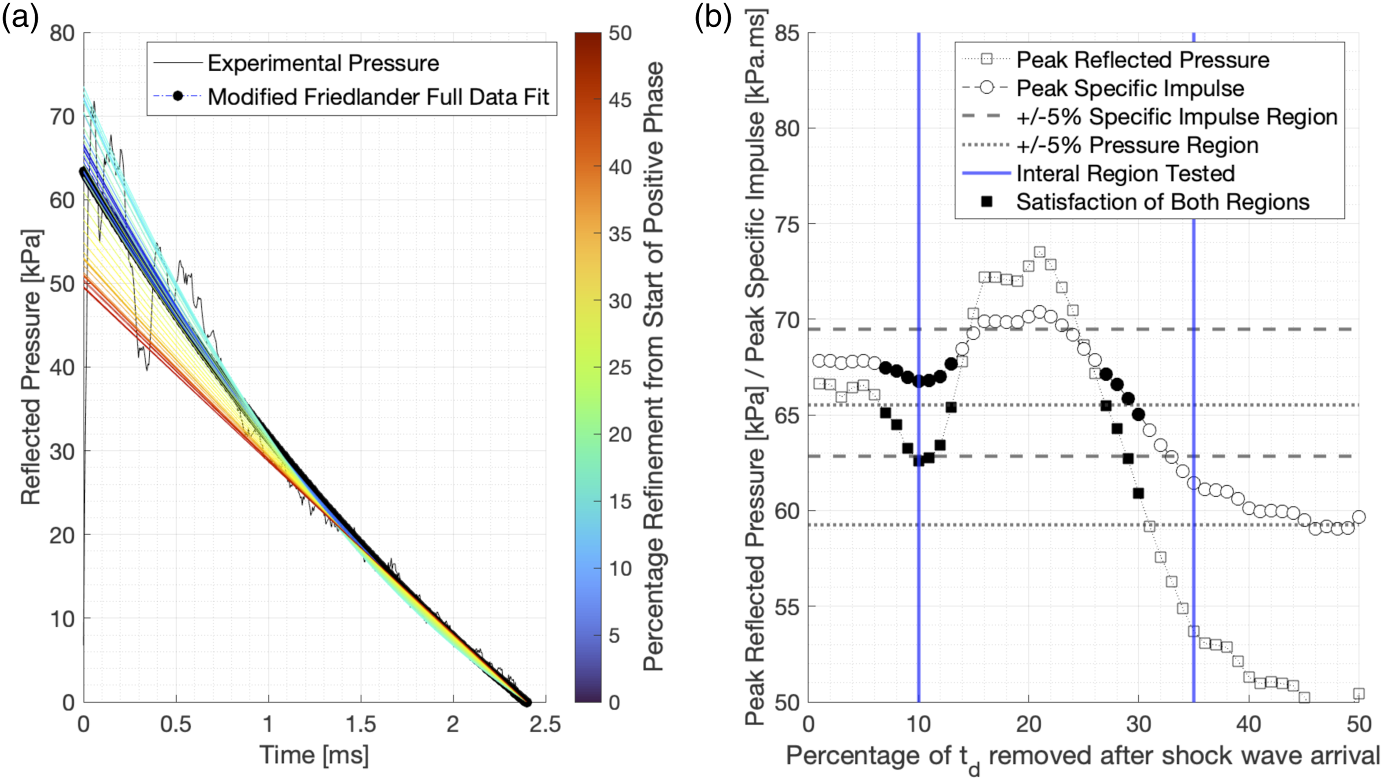

Figure 4(b) visually represents the peak pressures and specific impulse envelopes with respect to the percentage of t_d removed (from the start of the positive phase). The cyclic pattern in the opening 0–35%, and the fanning envelope introduced previously, is a result of fitting to different proportions of peaks and troughs in the electrical signal caused by sensor ringing. The reductions in both parameters after 35% represents the progressive loss of credible data and thus inaccuracies in representing features of the blast wave. The dip in peak pressure and specific impulse around 10% is as a result of fitting to the first major sensor ringing loss, seen for this test at t ≈ 0.3ms after arrival in Figure 4(a). A region of cyclic parameters was seen consistently at approximately 10–35% positive phase removal for all validation tests. Accordingly, this interval was set as the representative region over which the mean values were evaluated in step 4 of the algorithm, visually displayed by the vertical lines in Figure 4(b).

Step 4 assigns the most statistically representative parameters within this reduced region. First, the mean peak pressure and mean peak specific impulse between the entire region of 10–35% positive phase removal is calculated. Then, any percentage positive phase removal that results in a peak pressure or peak specific impulse deviating from this initial mean by more than 5% is discounted, and the mean values from each new, reduced dataset are calculated. This is shown visually in Figure 4(b), where the vertical lines denote the initial region where the first mean is taken (10–35%), the hollow markers indicate those that are excluded from the final mean calculation, and the solid markers indicate those data points that are included in the final mean calculation.

Finally, Figure 5(a) and (b) show the raw data from the example historic test (250 g PE4 hemisphere at 4 m stand-off), and the resulting modified Friedlander curve fits determined from the automated process. The high R² values noted on each figure show that the generalised model fits compare well to the raw data and therefore can be used with confidence to provide robust and accurate representations of the recorded explosive event. It is worth reiterating that although Figure 5(a) and (b) present optimal fits from a given test, they are evaluated from a large number of different potential fits. A secondary aim of this analysis was to confirm whether a consistent value of 0.25t_d removed after the arrival time was suitable as a general rule. Only 10 of the 65 validation trials resulted in optimum curves whose parameters were determined from trial fits outside of (0.25 ± 0.03)t_d, and this was mainly due to the level of sensor ringing that was present. With low levels of sensor ringing, the optimal amount of data removal was found to range between 0 and 0.2t_d, meaning that a Friedlander curve could effectively be fit to the entire data set without any loss of accuracy. For tests with intermediate to excessive sensor ringing, or for poor signal-to-noise ratios, a value of 0.25t_d is deemed suitable and can be used as a general rule in the absence of more sophisticated techniques such as the one presented in this article.

Figure 5.

Example historic test results using a 250g PE4 hemispherical charge at 4 m stand-off with optimal fits overlain: (a) Pressure, and; (b) Specific impulse.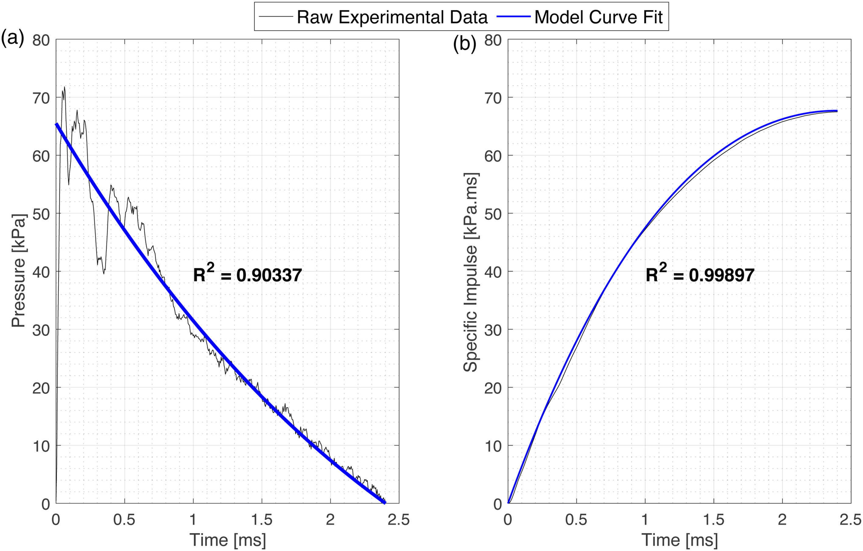

Compiled results

The optimal blast parameters determined from the automated process for the 65 PE4 trials used to validate the method (Rigby et al., 2014a), the additional 79 historical PE4 trials (Rigby et al., 2014b; Tyas et al., 2011) and the 10 current PE4 trials are presented in Figure 6(a)–(d) as a function of scaled distance. Positive phase duration (Figure 6(b)) was not determined in the historic tests and so are omitted here.

Figure 6.

Compiled blast parameters from PE4 trials as a function scaled distance, compared with KB predictions: (a) Scaled arrival time, (b) Scaled positive phase duration, (c) Peak reflected pressure, (d) Scaled reflected peak specific impulse.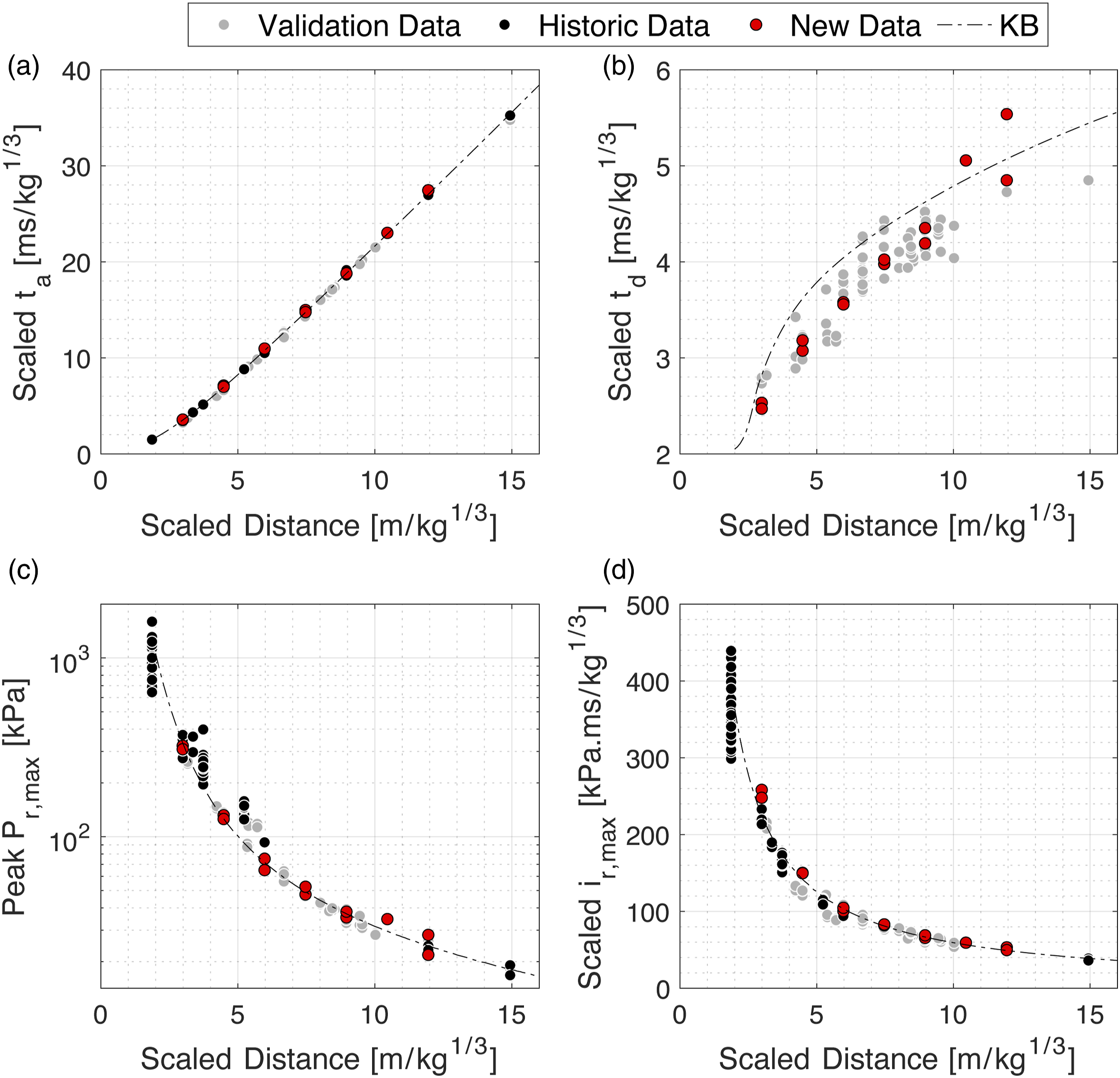

The data presented in Figure 6(a)–(d) have been expressed using the Hopkinson–Cranz scaling (Cranz, 1926; Hopkinson, 1915) assuming a constant TNT equivalence of PE4 of 1.20. For comparison, KB predictions have also been included in these figures. The recorded blast parameters demonstrate excellent agreement with the KB predictions, particularly in the region of Z > 4 m/kg ^1/3. The agreement between experiment and prediction is less good for Z < 4 m/kg^1/3, although the results are still typically within 10–20%. The cause in this deviation is currently unknown, but is likely due to irregular features of the fireball/air interface giving rise to non-consistent TNT equivalences in the mid- to near-field. This is the subject of ongoing work.

When considering test-to-test repeatability, there are two main conclusions to be drawn, both in agreement with findings published in the literature. Firstly, uncertainty in experimentally record blast parameters generally reduces with an increase in scaled distance (Bogosian et al., 2014; Rae and McAfee, 2018) seen mainly in Figure 6(c) and (d). Secondly, despite best efforts to remove unconscious researcher-dependent bias, peak pressure, specific impulse and positive phase duration, in nominally identical scenarios, demonstrate much higher levels of test-to-test variability than shock front arrival time. This can be seen when comparing Figure 6(b)–(d) with 6(a), respectively. It is suggested that test-to-test variations are non-negligible for Z < 3 m/kg^1/3.

Arrival time is considerably more repeatable than the other parameters. There is clear motivation to establish whether t_a is a consistent metric from nominally identical tests and whether it be recorded with enough accuracy to be used as an important diagnostic tool. The remainder of this article is focussed on quantification of variability in shock wave arrival time with respect to distance, and its relation to other blast parameter uncertainty.

HSV analysis

Procedure

Shock wave edge detection algorithms

Rigby et al. (2020a) presented an edge detection algorithm for explosive video recordings using HSV camera. The inbuilt MatLab function, edge (Canny, 1986), was suitable for optical tracking of the fireball/air interface in near-field explosive analysis due to the presence of a clear contrast between the luminous fireball and the ambient air. However, when testing the modified edge function for far-field scenarios the absence of a fireball in the images and low variations in light intensity across the shock front resulted in the most noticeable edges being those of the zebra board behind the shock front.

Hargather and Settles (2010) presented an image subtraction method which identifies the regions of greatest variation in pixel brightness between two consecutive frames. This method is particularly suited for situations with imagery of low contrast but with a clear schlieren disturbance (Gerasimov et al., 2017). A simplified approach based on this idea is presented in equation (2)

N_{i, j, k} = F_{i, j, k + 1} - F_{i, j, k}

(2)

where N is the resulting image subtracted video file, F the recorded video file, i and j are the pixel locations in terms of columns and rows, respectively, and k is the frame number. A comparison exercise was undertaken between the Hargather and Settles (2010) method and the simplified approach in equation (2) and the results were nominally identical for the videos tested. Despite the method being suited for low levels of lighting, weather conditions were particularly adverse in two of the 10 tests and therefore only eight videos yielded useful footage.

Whilst the method in the current paper has been shown to work well against a structured, repeatable background, other work using similar methods (Mizukaki et al., 2014) has been shown to yield accurate results with a highly variable ‘noisy’ background. The accuracy of this method for images with low contrast backgrounds has yet to be proven, however, it is envisaged that more sophisticated techniques (e.g. PIV) would be needed instead of the simple edge detection and image subtraction technique described herein.

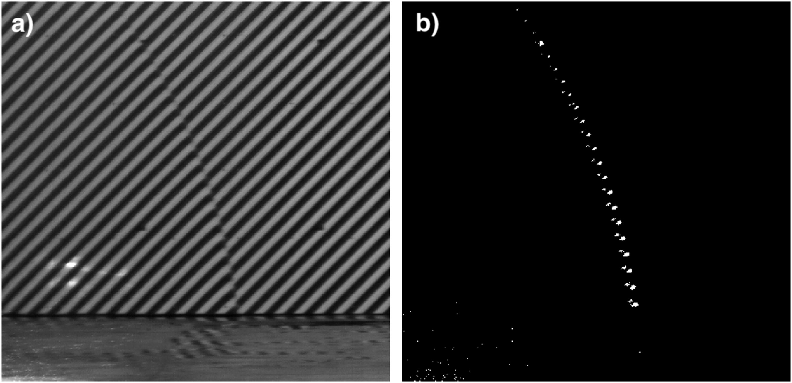
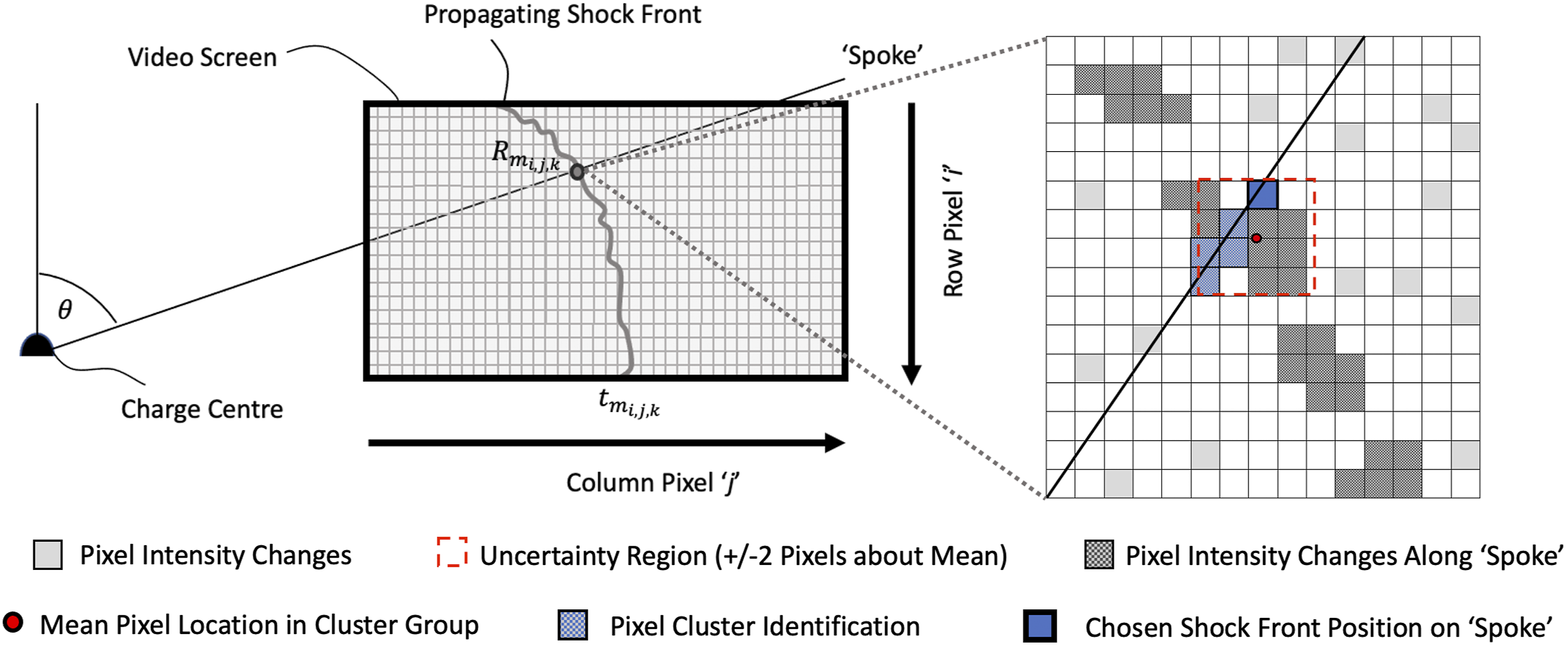
The results from a single frame of image subtraction are shown in Figure 7. A bespoke algorithm was written to accurately locate the propagating shock wave amongst random light variations between frames from the subtracted images. The algorithm consists of three stages: Pixel cluster identification, Intensity changes along radial spokes and Radial distance confirmation, the concept of which is shown Figure 8.

1. Pixel cluster identification: After eliminating any random light variation between subsequent frames, a clearly defined propagating shock wave can be identified by clusters of pixels, as seen in Figure 7(b). The clustering is related to the camera’s shutter speed, that is, lower frame rates resulted in an increased blurring effect. A MatLab script was written to locate the areas of each frame which had five or more connected pixels with large levels of light change in the image subtracted video, N. It is anticipated that with a higher frame rate, the number of connected pixels may reduce along with a more defined shock front, but five pixels was sufficient for all videos in this study.

2. Intensity changes along radial spokes: In a similar manner to previous studies (Rigby et al., 2020a), the second stage of the algorithm discretised the domain into 1° increments along virtual ‘spokes’. These span from the charge centre to the extents of the recording boundary. The location of any pixels which have light intensity changes along each ‘spoke’ are stored for each increment of angle and each frame. Due to the explosive charge being out of shot in each recording, the location was approximated through scaling-based calculations using the size of a pixel in the plane of the charge and known geometric relationships between the charge location, zebra board, camera and the pressure gauge in shot, following Gerasimov and Trepalov (2019) and Kucera et al. (2017). Fiducial markers on the zebra board, spaced 1.23 m horizontally and 1.33 m vertically, were used to calculate the corresponding pixel size of ∼3 mm for video resolution of 1024 × 560.

3. Radial Distance Confirmation: The pixel locations saved as a result of stage one and two were then compared directly to automate the shock front locating algorithm along each ‘spoke’ and remove any random light variation between frames. A MatLab script was written to compare stages one and two with an uncertainty region of ±2 pixels about the mean pixel location of the stage one results. This presented all the pixels which satisfied both stages of the analysis. To find the radial distance a given pixel is away from the charge, the locations of the camera, explosive and shock wave pixel location on the zebra board, denoted by subscript i, j and k, respectively, were set up with coordinates in 3D space, x, y and z. The distances between each of the three locations were calculated using equations (3)–(5), where a is the distance between the explosive and the camera, b is the distance between the explosive and pixel’s relative location on the zebra board, and finally c is the distance between the camera and the pixel’s relative location on the zebra board (see Figure 9 for reference)

a = \sqrt{{(x_{i} - x_{j})}^{2} + {(y_{i} - y_{j})}^{2} + {(z_{i} - z_{j})}^{2}}

(3)

b = \sqrt{{(x_{j} - x_{k})}^{2} + {(y_{j} - y_{k})}^{2} + {(z_{j} - z_{k})}^{2}}

(4)

c = \sqrt{{(x_{i} - x_{k})}^{2} + {(y_{i} - y_{k})}^{2} + {(z_{i} - z_{k})}^{2}}

(5)

Figure 7.

HSV stills from a test using 250 g PE4 hemisphere at 4 m stand-off: (a) Raw video footage, and; (b) Corresponding image subtraction.

Figure 8.

Method for detecting location of Shock Front through intensity changes on a virtual ‘spoke’ overlaid with pixel cluster identification.

Figure 9.

Schematic of shock wave radius calculation in 3D space to be used in conjunction with equations (3)–(7).

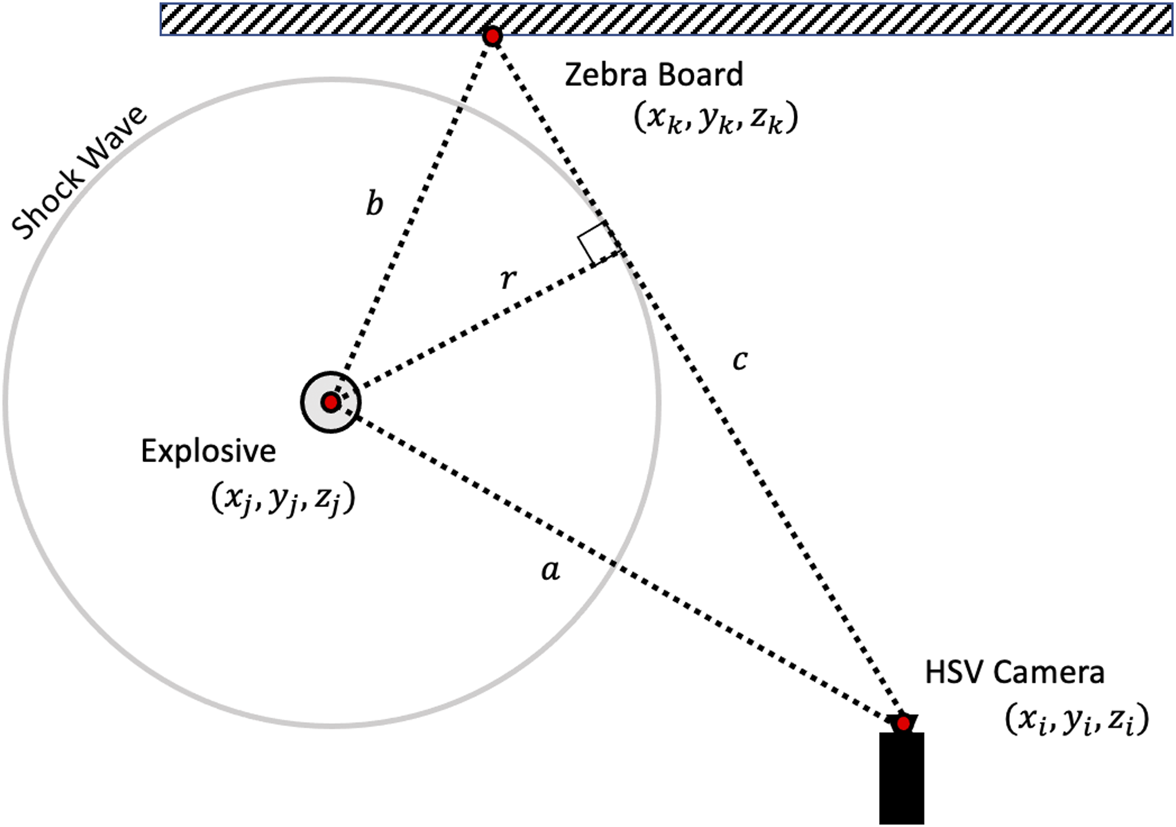
These distances were then used to calculate the area of the triangle, A, enclosed between the three points using Heron’s formula (equations (6) and (7)). Assuming that the shock wave is expanding spherically, and the line between the camera and the shock wave pixel location is a tangent to the sphere, and therefore the radius, r, of the shock would be equal to the height of the triangle, abc

A = \sqrt{(s (s - a) (s - b) (s - c)}

(6)

s = \frac{a + b + c}{2}

(7)

r = \frac{2 A}{c}

(8)

After calibrating, the pixel furthest away from the charge centre was identified as the position of the shock front along a particular ‘spoke’, at a given time. This was done to achieve test-to-test consistency regardless of the frame rate and associated blurring. It is important to note that although strict experimental procedures were in place, focal lengths were difficult to record as a manual zoom was used. Despite the levels of zoom being consistent, lens distortion effects subsequently were not accounted for during each test and thus would cause minor variations between videos recording different stand-off distances. Previous research has suggested that lens distortion results in minimal levels of uncertainty in pixel size calibration (Robbe et al., 2014). In the current study, lens distortion was minimised by comparing only like-for-like tests.

Example of edge detection algorithm

The results from the edge detection algorithm for a single test (250 g PE4 hemisphere at 5 m stand-off) are presented in Figure 10. Also shown are KB predictions, again using Hopkinson–Cranz scaling and a TNT equivalence of 1.20. The high levels of agreement highlights the repeatability and accuracy in the results from the presented automated image tracking and arrival time interpolation algorithms. When comparing Figures 6(a) and 10, the full-field data extracted from a single video gives a clear justification for the use of HSV over pressure gauges when studying shock wave arrival time.

Figure 10.

Shock front arrival time from a 250 g PE4 hemispherical charge placed at a 5 m stand-off, recorded using HSV and scaled using 1.20 TNT equivalence factor to compare to KB predictions.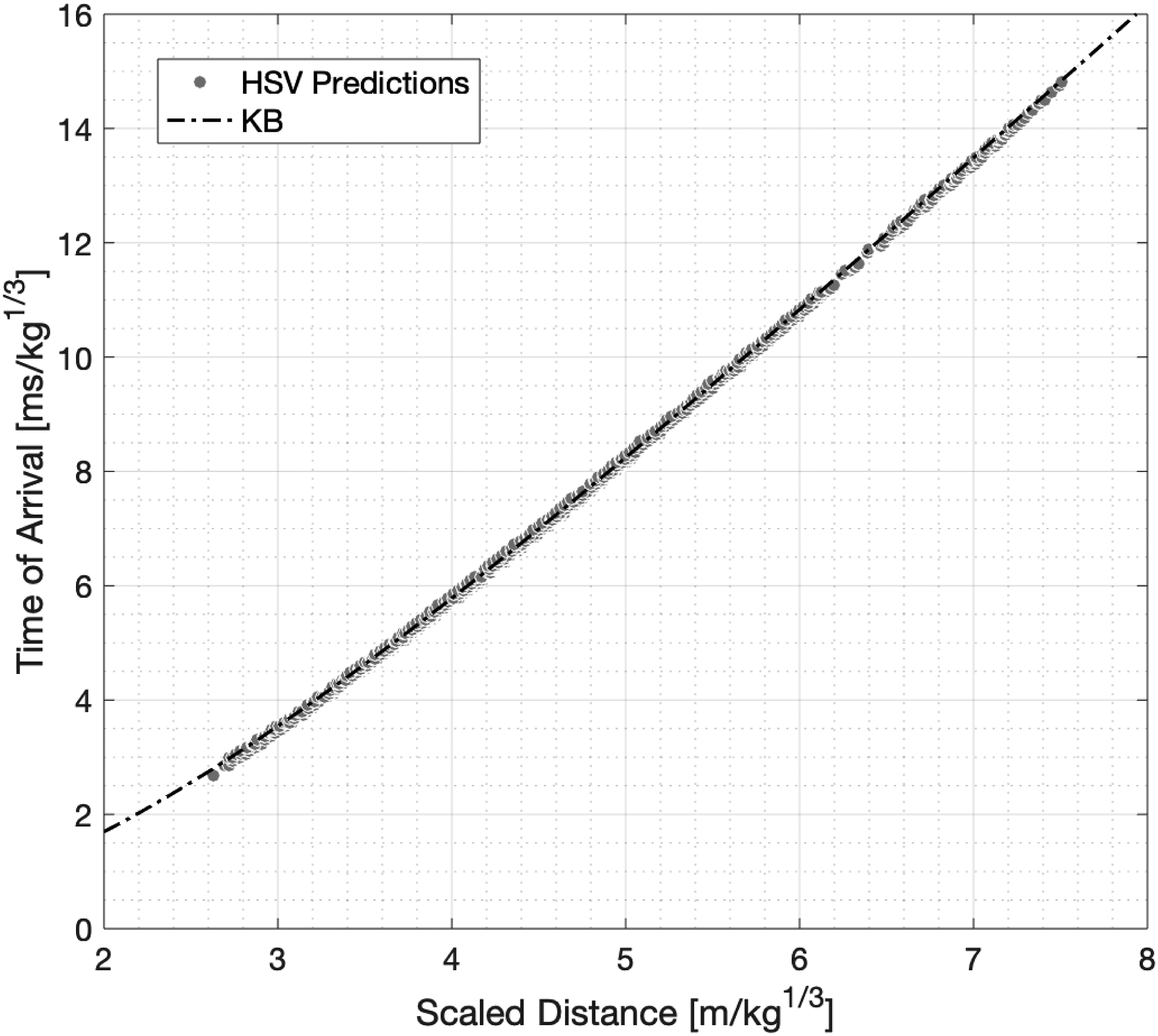

Shock wave arrival time interpolation

Blast parameters such as peak incident and reflected pressure can be linked to shock velocity (Mach number) through the well-known Rankine–Hugoniot jump conditions (Kinney and Graham, 1985). There is motivation, therefore, to understand how blast wave arrival time (thus Mach number) varies with changing distance from the centre of the explosive, as this has implications on the inherent variability of pressure and impulse parameters also.

A method, presented visually in Figure 11, was proposed to interpolate arrival time data at increments of 0.1 m/kg^1/3 scaled distance along each virtual ‘spoke’ for each HSV recording. In doing this, a direct comparison could be made between pressure gauge recordings of arrival time, with discrete scaled distances, and HSV recordings with discrete increments of time between each frame but a variety of processed distances.

Figure 11.

Method of interpolation of shock front arrival times along a virtual ‘spoke’ for prescribed scaled distances.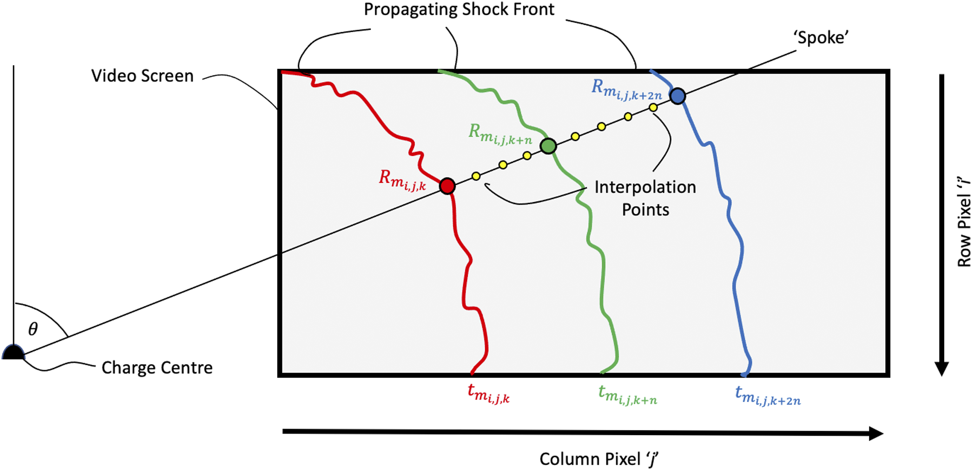

The interpolated arrival times were collated with respect to scaled distance, and the relative standard deviations (RSTD, σ/μ) calculated to express the precision and repeatability of HSV arrival time recordings. For each of the eight HSV recordings, scaled distances ranged between 2.4 and 12.3 m/kg^1/3. Discretising the domain into 1° radial spokes enabled the propagating shock front position from the charge centre to be identified along a radial virtual line, with respect to time.

The presented interpolation method when used on the eight HSV recordings resulted in 3012 different interpolated arrival times, all with their corresponding scaled distances. When collating the videos by nominally identical arrangements, between 5 and 31 independently interpolated t_a values were obtained for each increment of scaled distance tested.

Discussion

Pressure gauge measured TOA variability

Despite the visibly low levels of variability shown in Figure 6(a), shock front time of arrival, t_a, is a somewhat overlooked parameter when compared to peak pressure and peak specific impulse. The main aim of this article is to investigate and quantify the variability of shock wave arrival times, and investigate how this varies with scaled distance is required.

Initially, RSTD was calculated from the pressure gauge arrival time data (from the historic and current tests presented in this article, 157 in total). The results can be used assess variations in the measurements from this particular method and are presented in Figure 12.

Figure 12.

Relative standard deviation in shock wave arrival time with respect to scaled distance, from historic and current pressure gauge data.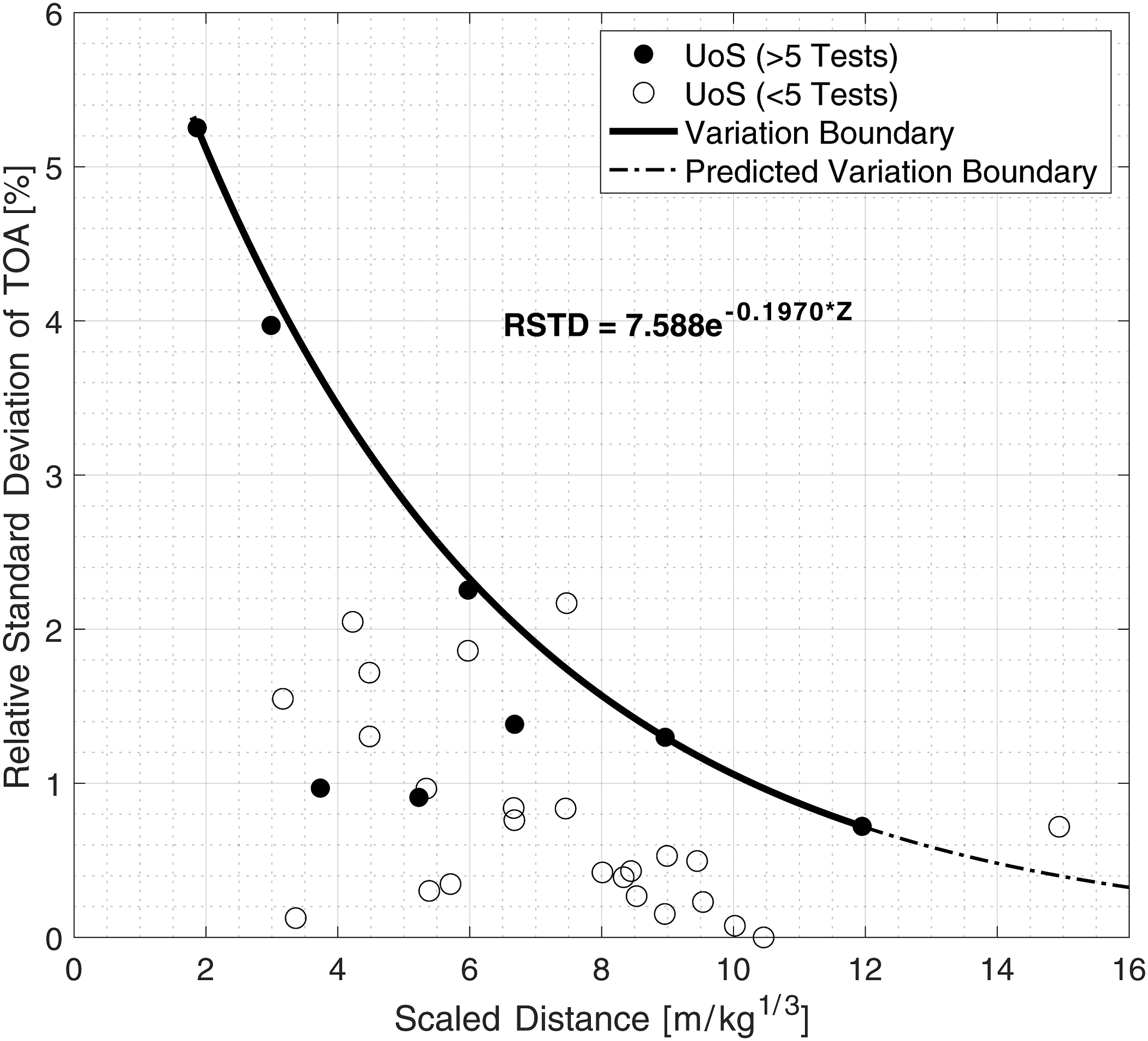

Of the scaled distances tested, a small number contain data from at least five nominally identical tests. These are shown in Figure 12 as solid markers, and a clear exponential trend connects them. All other scaled distances had less than five repeat tests and are omitted from this fit, however, are still shown as hollow markers and demonstrate the same qualitative behaviour: decreasing variability with increasing scaled distance.

This supports the idea of instabilities in the shock front forming and diminishing, thus causing variability, in the intermediate range of scaled distances. The exponential relationship has been defined for the region of scaled distances tested and extrapolated as a guideline prediction outside these ranges. Future works will look at testing near-field conditions, Z < 2m/kg^1/3, in the hope to show a reduction in arrival time variability associated with a smooth shock front before instabilities start to form, in the support of the hypothesis of shock wave instability regions (Tyas, 2019). The important point to address is that quantifying t_a variability related to scaled distance, which can be chosen with little ambiguity, provides a further insight into the development of a shock front form and resulting undulations. Current predictive methods provide discrete blast parameters for a given scaled distance an explosive is away from a target. Through understanding the spread of experimentally measured t_a, improvements can be made to fast-running predictive methods to provide probabilistic blast parameters within the uncertainty range for a given distance.

HSV measured time of arrival variability

Following the edge detection at each frame across the entire video, the ‘spoke’ interpolation method was used to evaluate t_a values for specified increments of scaled distances. These were then collated and the RSTD calculated with respect to each increment of scaled distance. The standardised range of interpolated HSV arrival time results are presented in Figure 13, and compared directly to pressure gauge variation, with respect to scaled distance. A significant reduction in the variability of processed arrival times across the entire range of tested distances is seen when using HSV. In part, this reduction in variability is associated with the volume of data points created through the interpolation at each scaled distance. However, some of the scaled distances in question had a similar benchmark number of data points as the pressure gauge results. That being said, there is still a noticeable reduction in processed t_a variability. This alone provides clear justification for the use of video recordings during explosive trials to enhance the precision and repeatability of blast parameters between tests.

Figure 13.

Logarithmic Relative standard deviation in shock wave arrival time as a function of scaled distance for both pressure gauge and high-speed video recordings.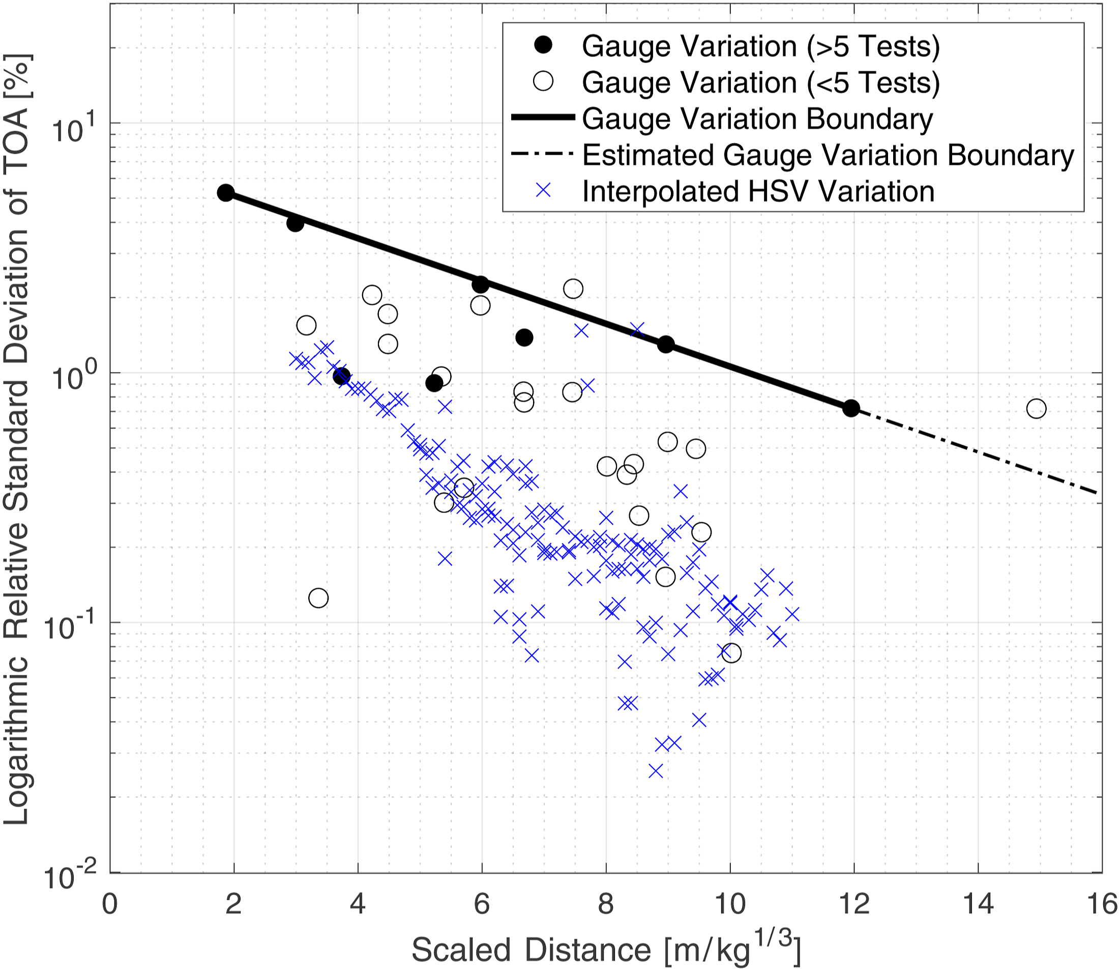

As lens distortion was not accounted for in this research, the videos were not used as a group of collated data and only those with the same test set up were compared. Regardless of this, the relative variability of arrival time recordings at specific scaled distances held fairly consistent between groupings of tests. One thing to note is the substantial volume of interpolated data from just 10 processed videos when compared to 157 different pressure gauge recordings. The larger data set (3012 recordings), alongside the clear improvement in repeatability and accuracy from just 10 explosive trials recorded using high speed cameras, presents a more cost-effective solution to experimental testing of high explosives.

The significance of Figure 13 is the comparable relationship between t_a variation with respect to scaled distance for both HSV and pressure gauge recordings. This is shown on a logarithmic scale to enable a more clear comparison between the processed results from both methods of recording. A clear exponential reduction in t_a variability is seen with an increase in scaled distance across both methods of experimental analysis, and the typical variations in the HSV data are approximately an order of magnitude lower than those in the pressure gauge data.

In summary, optically recorded t_a has been shown to exhibit markedly lower variations when compared to t_a determined from pressure gauge data, and considerably lower variations compared to directly measured peak pressures and specific impulses.

Derivation of explosive yield from arrival time data

To consider arrival time data as a metric for forensic explosive analysis, it is important to validate it against empirical data alongside quantifying the variability in the parameter. Rigby et al. (2020b) and Dewey (2021) both present methods of quantifying the explosive yield of a real-world accidental explosion through arrival time data analysis with respect to best estimations of stand-off from the explosive centre. Their findings presented clear agreement of explosive yield and thus the TNT equivalence factor of the explosive detonated.

To verify the shock wave tracking and interpolation algorithm as an accurate means of gaining an understanding of how arrival time varies spatially across a full range of scale distances, the method was tested to estimate the apparent yield of the explosive used during the tests, which is known to be 250 g PE4.

Figure 14 shows how the HSV-measured values of arrival time compare to a variety of different sized TNT charges and their corresponding KB predictions. It is important to note that the axes have been scaled down to visualise a clear distinction between the predictive TNT curves due to modest changes in charge mass. The HSV data shows excellent agreement with the curves for TNT between 290 and 320 g, equating to a TNT equivalence of 1.16–1.28. The minimum mean absolute error is associated with a TNT mass of 305 g, that is, an equivalence of 1.22, which is very close to the value of 1.20 found in related studies (Rigby and Sielicki, 2014). This suggests that the optical technique presented in this paper is a reliable method for determining the TNT equivalence of explosives.

Figure 14.

Interpolated and unscaled HSV shock wave arrival time from a 250 g PE4 hemispherical charge at 5 m stand-off compared with KB predictions for TNT hemispherical charges with different charge mass.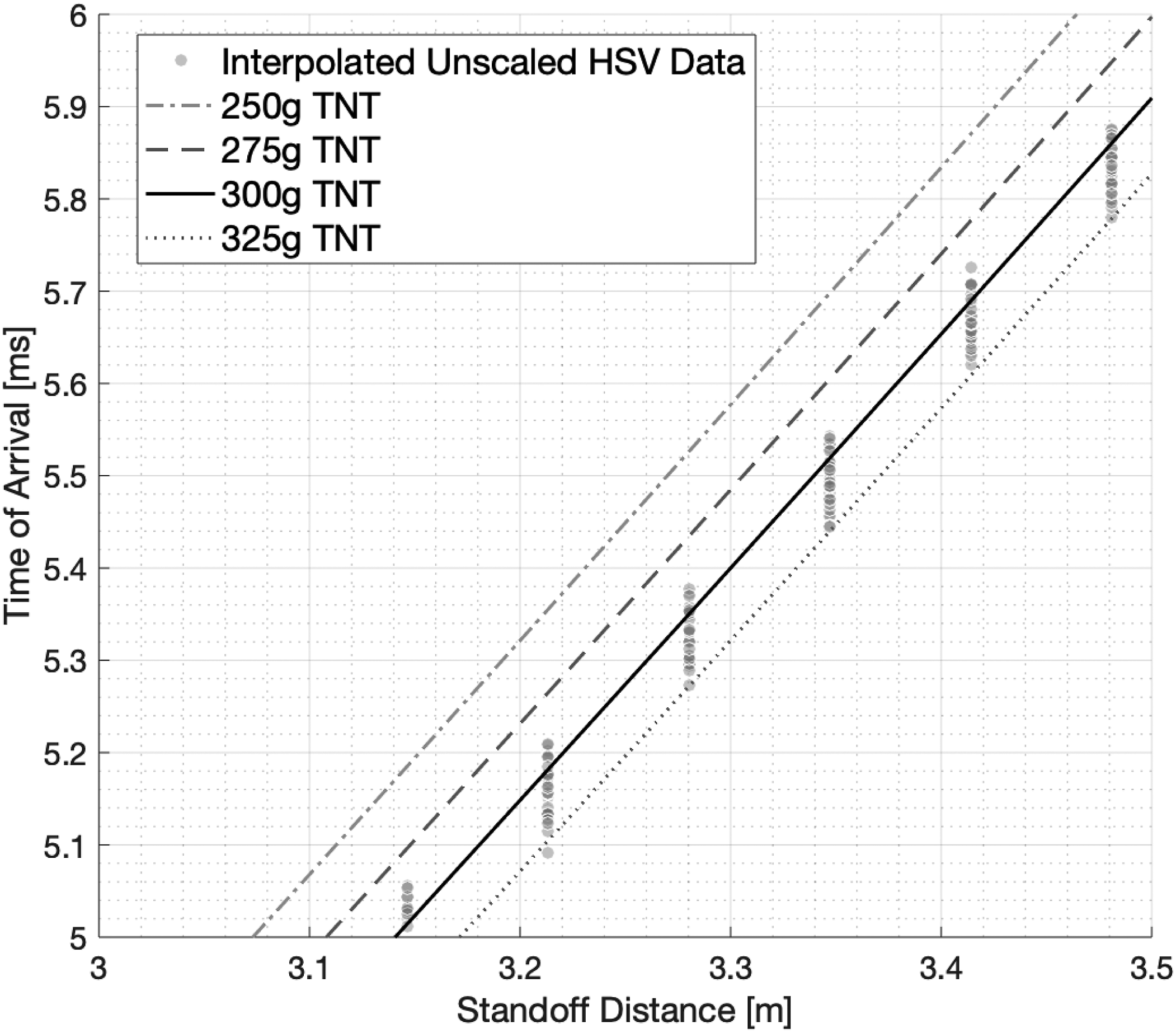

Conclusions and future work

This article presents a study on time of arrival as a diagnostic for far-field high explosive blasts using the results from 144 historic arena-style tests using surface-mounted pressure gauges, and 10 newly performed experiments using both pressure gauges and HSV.

Firstly, a method for automatically processing pressure gauge data is presented. As a general rule, removal of the first 25% of the positive phase duration and fitting a modified Friedlander curve to the remainder of the signal will negate the effects of sensor ringing and result in reliable determination of peak reflected pressure, peak specific impulse and decay coefficients. The results were compiled and compared against Kingery and Bulmash (1984) predictions and excellent agreement was demonstrated, particularly for Z > 3 m/kg^1/3. Noticeably, time of arrival demonstrated considerably less spread than positive phase duration, peak reflected pressure and peak specific impulse.

Secondly, a new routine for optically tracking a shock front was proposed, which enables the arrival time to be evaluated at regular distances from the explosive centre, permitting comparison between different tests. The new algorithm was used to determine full-field arrival times for the newly performed tests within this article. A clear exponential decrease in arrival time variability (RSTD) was observed. Furthermore, the arrival times determined from the HSV analysis demonstrated considerably lower variability, approximately an order of magnitude, than the results obtained from the pressure gauge data alone.

Finally, the results were used to verify the concept of using HSV arrival times to calculate the yield of high explosives. The results from this analysis were in very close agreement with established values of TNT equivalence (1.22 compared to 1.20) and therefore prove the viability of the method.

Time of arrival is shown to be a vital diagnostic tool in understanding and quantifying the typical variations seen in explosive blast testing, and can be used as a reliable source to investigate the origins of such variations.

Supplemental Material

sj-xlsx-1-prs-10.1177_20414196211062923 - Supplemental Material - Time of arrival as a diagnostic for far-field high explosive blast waves

Supplemental Material, sj-xlsx-1-prs-10.1177_20414196211062923 for Time of arrival as a diagnostic for far-field high explosive blast waves by Dain G. Farrimond, Sam E. Rigby, Sam D. Clarke and Andy Tyas in International Journal of Protective Structures

Footnotes

Acknowledgements

The authors wish to thank the technical staff at Blastech Ltd. for their assistance in conducting the experimental work.

Declaration of conflicting interests

The author(s) declared no potential conflicts of interest with respect to the research, authorship, and/or publication of this article.

Funding

The author(s) disclosed receipt of the following financial support for the research, authorship, and/or publication of this article: Experimental work reported in this paper was funded by the Engineering and Physical Sciences Research Council (ESPRC) as part of the Mechanisms and Characterisation of Explosions (MaCE) project, EP/R045240/1. The first author gratefully acknowledges the financial support from the EPSRC Doctoral Training Partnership.

ORCID iD

Sam E. Rigby

Supplementary data

Compiled blast parameters from historic and newly-performed tests have been included have been included as supplementary data.

References

Anderson

Parry

Ritzel

(2016) Time dependent blast wave properties from shock wave tracking with high speed video. In: 24th international symposium on military aspects of blast and shock (MABS), Halifax, Nova Scotia, Canada, 18–23 September

Baker

(1973) Explosions in Air. Austin: University of Texas Press.

Biss

McNesby

(2014) Optically measured explosive impulse. Experiments in Fluids 55(6): 1749.

Bogosian

Ferritto

Shi

(2002) Measuring uncertainty and conservatism in simplified blast models. In: 30th Explosives Safety Seminar, Atlanta, GA, USA, 13–15 August

Bogosian

Powell

Ohrt

(2019). Consequences of Applying Objective Methods for Selecting Peak Pressure from Experimental Data. In: Internationl symposium of the interaction of effects of munitions with structures (ISIEMS), Panama City, Florida, 21–25 October, p. 11.

Bogosian

Dailey

, et al. (2014) Statistical variation in reflected airblast parameters from bare charges. In: 23rd international symposium on military aspects of blast and shock MABS), Oxford, England, 7–12 September.

Canny

(1986) A computational approach to edge detection. IEEE Transactions on Pattern Analysis and Machine Intelligence 8(6): 679–698.

Clarke

Fay

Warren

, et al. (2014) A large scale experimental approach to the measurement of spatially and temporally localised loading from the detonation of shallow-buried explosives. Journal of Measurment Science and Technology 26(1): 015001.

Cranz

(1926) Lehrbuch der Basllistik. Berlin: Springer Germany.

10.

Dewey

(1971) The properties of a blast wave obtained from an analysis of the particle trajectories. Proceedings of the Royal Society of London. A. Mathematical and Physical Sciences 324(1558): 275–299.

11.

Dewey

(2021) The TNT and ANFO equivalences of the Beirut explosion. Shock Waves 31: 95–99.

12.

Esparza

(1986) Blast measurements and equivalency for spherical charges at small scaled distances. International Journal of Impact Engineering 4(1): 23–40.

13.

Gerasimov

Mikhailov

Trepalov

, et al. (2017) Shock wave distribution in an explosion of an explosive material with plastic filler. Combustion, Explosion and Shock Waves 53: 689–695.

14.

Gerasimov

Trepalov

(2019) Video recording of an air blast wave resulting from initiation of a light-sensitive explosive composition. Combustion, Explosion and Shock Waves 55(5): 606–612.

15.

Hargather

(2013) Background-oriented schlieren diagnostics for large-scale explosive testing. Shock Waves 23(5): 529–536.

16.

Hargather

Settles

(2010) Natural-background-oriented schlieren imaging. Experiments in Fluids 48(1): 59–68.

17.

Hopkinson

(1915) British Ordnance Board Minutes. 13565 edn. Kew, UK: The National Archives.

18.

Hyde

(1991) Conventional Weapons Program (ConWep). USA: US Army Waterways Experimental Station, Vicksburg, MS.

19.

Igra

Seiler

(2016) Experimental Methods of Shock Wave Research. Switzerland: Springer International Publishing.

20.

Kennedy

(1946) Explosions and explosives in air. In: Effects of Impact and Explosions. Summary Technical Report of Div. 2. Washington, DC, AD 221 586: NDRC, Vol. 1.

21.

Kingery

Bulmash

(1984) Airblast Parameters from TNT Spherical Air Burst and Hemispherical Surface Burst. MD, USA: ARBRL-TR-02555, US Army Ballistic Research Laboratory, Aberdeen Proving Ground.

22.

Kinney

Graham

(1985) Explosive Shocks in Air. Springer-Verlag Berlin Heidelberg.

23.

Kucera

Anastacio

Selesovsky

, et al. (2017) Testing optical tracking of blast wave position for determination of its overpressure. In: 6th international conference on military technologies (ICMT), Brno, Czech Republic, 31st May–2nd June, pp. 70–73.

24.

Lyons

(2012) Characteristation of Blast Wave Variability. PhD thesis, Australia, The University of Newcastle.

25.

Meshkov

(1969) Instability of the interface of two gases accelerated by a shock wave. Fluid Dynamics 4(5): 101–104.

26.

Mizukaki

Wakabayashi

Matsumura

, et al. (2014) Background-oriented schlieren with natural background for quantitative visualization of open-air explosions. Shock Waves 24(1): 69–78.

27.

Nansteel

Veldman

Chen

CC-T

, et al. (2013) Impulse plug measurements of blast reflected impulse at close range. Propellants, Explosives, Pyrotechnics 38(1): 120–128.

28.

Netherton

Stewart

(2010) Blast load variability and accuracy of blast load prediction models. International Journal of Protective Structures 1(4): 543–570.

29.

Ohashi

Kleine

Takayama

(2001) Characteristics of blast waves generated by milligram charges. In 23rd international symposium on shock waves, Fort Worth, USA, 22–27 July, pp. 187–193.

30.

Ohrt

Dailey

Bogosian

(2014) Statistical variation of airblast parameters from bare and cased explosive cylinders. In ‘22nd international symposium on military aspects of blast and shock (MABS)’, Bourges, France, 4–9 November.

31.

Pontalier

Loiseau

Goroshin

, et al. (2021) Blast enhancement from metalized explosives. Shock Waves 31: 203–230.

32.

Rae

McAfee

(2018) The blast parameters spanning the fireball from large hemispherical detonations of C-4. Propellants, Explosives, Pyrotechnics 43(7): 694–702.

33.

Randers-Pehrsons

Bannister

(1997) Airblast Loading Model for DYNA 2D and DYNA 2D, Technical Report ARL-TR-1310 . Aberdeen Proving Ground, MD, USA.

34.

Rayleigh (1882) Investigation of the character of the equilibrium of an incompressible heavy fluid of variable density. Proceedings of the London Mathematical Society s1-s14(1): 170–177.

35.

Richtmyer

(1960) Taylor instability in shock acceleration of compressible fluids. Communications on Pure and Applied Mathematics 13(2): 297–319.

36.

Rickman

Murrell

(2007) Development of an improved methodology for predicting airblast pressure relief on a directly loaded wall. Journal of Pressure Vessel Technology, Transactions of the ASME 129(1): 195–204.

37.

Rigby

(2021) Blast Wave Time of Arrival : A Reliable Metric to Determine Pressure and Yield of High Explosive Detonations, Technical Report 079, Fire and Blast Information Group.

38.

Rigby

Fay

Tyas

, et al. (2015) Angle of incidence effects on far-field positive and negative phase blast parameters. International Journal of Protective Structures 6(1): 23–42.

39.

Rigby

Gitterman

(2016), Secondary shock delay measurements from explosive trials. In: ‘24th international symposium on military aspects of blast and shock (MABS)’, Halifax, Nova Scotia, Canada, 18–23 September.

40.

Rigby

Knighton

Clarke

, et al. (2020a) Reflected near-field blast pressure measurements using high speed video. Experimental Mechanics 60(7): 875–888.

41.

Rigby

Lodge

Alotaibi

, et al. (2020b) Preliminary yield estimation of the 2020 Beirut explosion using video footage from social media. Shock Waves 30(6): 671–675.

42.

Rigby

Sielicki

(2014) An investigation of TNT equivalence of hemispherical PE4 charges. Engineering Transactions 62(4): 423–435.

43.

Rigby

Tyas

Bennett

, et al. (2014b) The negative phase of the blast load. International Journal of Protective Structures 5(1): 1–19.

44.

Rigby

Tyas

Fay

, et al. (2014a), Validation of semi-empirical blast pressure predictions for far field explosions - is there inherent variability in blast wave parameters? In: ‘6th international conference on protection of structures against hazards’, Tianjin, China, 16–17 October, pp. 1–9.

45.

Robbe

Nsiampa

Oukara

, et al. (2014) Quantification of the uncertainties of high-speed camera measurements. International Journal of Metrology and Quality Engineering 5: 201–209.

46.

Schoutens

(1979) Review of Large HE Charge Early-Time Detonation Anomalies. Washington, DC: Technical Report DASIAC SR 182.

47.

Smith

Rose

Saotonglang

(1999) Clearing of blast waves from building facades. Proceedings of the Institution of Civil Engineers: Structures and Buildings 134(2): 193–199.

48.

Tang

Bird

Rigby

, et al. (2017) Reflections on variability of blast pressure measurement at different scales. In: ‘17th international symposium on the interaction of the effects of munitions with structures’, Bad Neuenahr-Ahrweiler, Germany, 16–20 October.

49.

Tang

Rigby

Tyas

(2018) Validation of Air3D for scaled experimental pressure and impulse data. In: ‘25th international symposium on military aspects of blast and shock (MABS)’, The Hague, Netherlands, 24–27 September.

50.

Taylor

(1950) The instability of liquid surfaces when accelerated in a direction perpendicular to their planes. II. Proceedings of the Royal Society of London. Series A. Mathematical and Physical Sciences 202(1068): 81–96.

51.

Tyas

(2019) Blast loading from high explosive detonation: what we know and don’t know. In: ‘13th international conference on shock and impact loads on structures (SILOS)’, Guangzhou, China, 1365-1576 December, pp. –.

52.

Tyas

Reay

Fay

, et al. (2016) Experimental studies of the effect of rapid afterburn on shock development of near-field explosions. International Journal of Protective Structures 7(3): 452–465.

53.

Tyas

Warren

Bennett

, et al. (2011) Prediction of clearing effects in far-field blast loading of finite targets. Shock Waves 21(2): 111–119.

54.

US Department of Defence (2008) ‘Structures to Resist the Effects of Accidental Explosions’. UFC 3-340-02. Washington, DC: US DoD.

Supplementary Material

Please find the following supplemental material available below.

For Open Access articles published under a Creative Commons License, all supplemental material carries the same license as the article it is associated with.

For non-Open Access articles published, all supplemental material carries a non-exclusive license, and permission requests for re-use of supplemental material or any part of supplemental material shall be sent directly to the copyright owner as specified in the copyright notice associated with the article.

0.00 MB

0.03 MB