Investigation of rope formation in gas–solid flows through a 90° pipe bend using high-speed video and CFD simulations

Abstract

A study of rope formation in gas–solid flows through abrupt turns has been conducted. Experiments in which high-speed video was recorded and analyzed for solid concentration profiles were compared to CFD simulations utilizing both RANS and large eddy simulation turbulence models. In both simulations and experiments, particle-laden flows of air and ground flaxseed, with solid loadings of 35, 42, and 51% were considered. The results of the study demonstrate that both RANS and large eddy simulation can accurately predict particle roping. Furthermore, simulations show that the roping phenomenon is strongly dependent upon selection of an appropriate value for the coefficient of restitution. Additionally, a strong relation between local solid concentration and gas vorticity was observed.

Introduction

The pneumatic conveying of solids is a ubiquitous process that is used over a wide range of industries, including the chemical, pharmaceutical, food processing, and power generation. ¹ For example, in a pulverized coal power plant, coal fines are pneumatically transported to the combustors via a network of pipes. These piping systems will include several sharp 90° bends, or elbows, which provide a considerable amount of flexibility for routing and distributing the conveyed material throughout a plant, but are one of the primary factors affecting the nature of the gas–solid flow within the piping system. ² As the air and coal mixture passes through these elbows, inertial effects and pipe geometry cause the formation of rope-like structures. The ropes carry the bulk of the transported material concentrated within a small cross-section of the pipe, typically with lower particle velocities and relatively high solid concentrations. ¹ Consequently, an acceleration region downstream of the pipe elbow is required to reaccelerate the entrained solids back to the velocity of the conveying gas. ² The formation and disintegration of these flow-related structures is a complex phenomenon that is affected by many factors, including: centrifugal forces, secondary flows, gas velocity, pipe geometry, and physical properties of the transported solid. The presence of these ropes lead to problems with flow control and measurement within the power plant and are widely believed to adversely affect the ability to reduce NO_X emissions and lead to increased levels of unburnt carbon in the fly ash. ³ Therefore, significant efforts have been devoted to understanding the mechanisms that cause rope formation, as well as how to mitigate and/or predict the formation of particle roping. While the majority of the literature available regarding rope formation is associated with transport of coal fines, it is an issue that can affect any pneumatically transported particulate.

Yilmaz and Levy ³ studied the formation of ropes by coal fines through a 90° elbow transitioning from horizontal to vertical (upwards) pipe flow for an air-to-solid loading ratio of 1. They used a fiber optic probe to measure particle velocities and concentrations, generating radial profiles for each. Their results showed that ropes would form and initially move towards the outer wall of the pipe bend, and then later be brought back towards the mid-section of the pipe by secondary flows, where the ropes would then be dispersed by flow turbulence. Furthermore, they found that the dispersal of these rope formations could be accelerated by the introduction of an orifice plate into the flow. In a later study, Yilmaz and Levy ¹ conducted experiments to examine the effects of different elbow radius of curvature/pipe diameter (R/D) ratios on rope formation and dispersion. In addition, they performed simulations using a commercial CFD package (CFX-Flow3D) utilizing an Eulerian-Lagrangian approach with a two-equation k–ɛ turbulence model. They found that their experiments showed a strong effect of the R/D ratio on the rate of rope dispersal. The higher the R/D ratio, the slower the rate of dispersal. They reported that not only did the CFD model not show this behavior but the CFD results also overpredicted the peak particle concentrations within the rope at the elbow exit, concluding that this was most likely due to the absence of particle–particle interactions within the CFD model. Akilli et al. ² studied rope formation in a vertical-to-horizontal elbow, finding that strong ropes would fully disperse within 10 pipe diameters of the elbow exit, and that fully developed concentration and velocity profiles were obtained within 30 pipe diameters of the elbow exit. They also found the rope formation to be highly dependent upon the R/D ratio. Simulations performed by Akilli et al. (using the same models as Yilmaz and Levy) showed that secondary flow structures would disperse the ropes by carrying the fine particles around the pipe circumference, and that average particle diameter contours indicated that the average particle size was larger in the rope than elsewhere in the pipe cross section. Kruggel-Emden and Oschmann ⁴ studied the effects of various particle shapes on rope dispersion in a horizontal-to-vertical (upwards flow) elbow using coupled DEM-CFD simulations. Their results indicated that the rate of rope dissipation was strongly affected by particle shape, where icosahedrons provided the most rapid rope dispersion and plates the lowest. They went on to observe the general trend that strong particle–fluid interaction, particle–particle collisions and large bend exit velocities result in accelerated rope dispersion. Guda et al. ⁵ presented a model validation study as well as a study on rope formation in a vertical to horizontal elbow using both ground flaxseed and high-density polyethylene (HDPE) pellets for a variety of particle size distributions and found that the preliminary simulation results obtained from using a Reynolds Averaged Navier-Stokes (RANS) model in Fluent failed to accurately predict the onset of roping with HDPE pellets at a solid-to-gas loading ratio of less than 1.5. In their study, the simulation results suggested the presence of rope formation for solid-to-air loadings which did not result in roping under experimental conditions, thus pointing to a need for model refinements to more accurately predict roping behavior. (As will be demonstrated later, the authors of the current work believe that the coefficient of restitution used in Guda et al. ⁵ to be insufficient.)

The authors of the current study believe that the primary reason for the reported discrepancies between experimental observations and simulations deems further study on the primary factors which affect the roping phenomenon and hence elucidate why many previous authors claim that state-of-the-art CFD models fail to capture it adequately. The factors that are considered are turbulence models and a strong model dependence upon the value of the coefficient of restitution. Moreover, the current study employs a unique and quick measurements technique utilizing high-speed video, and demonstrates that when applied in parallel it could be very effective.

Experimental setup

System description

For this study, the experimental setup shown in Figure 1 was used to obtain high-speed video data of roping under different loading conditions. The experimental unit consists of a vertical pipe section, a 90° vertical-to-horizontal elbow, and then a horizontal pipe section. The vertical pipe section is composed of a 2.5 in. (6.35 cm) inner diameter clear acrylic tube that is 36 in. (91.44 cm) in length, above the acrylic tube is a 3 in. (7.62 cm) inner diameter borosilicate glass pipe section that is 12 in. (30.48 cm) in length. The borosilicate glass elbow has a 3 in. inner diameter and a radius of curvature to pipe diameter ratio (r/d) of 1.8. The horizontal section consists of a 3 in. inner diameter × 36 in.-long borosilicate glass pipe, followed by a 2.5 in. diameter by 36 in. long clear acrylic tube. The outside diameter of the acrylic tubes for both the vertical and horizontal sections was machined down on the ends to allow the tubes to fit inside the borosilicate glass pipes. These joints were sealed to prevent air leakage. The inside diameters of the ends of the acrylic tubes were also machined to allow smooth transition from the 2.5 in. diameter of the acrylic to the 3 in. diameter of the glass sections. A screw feeder was used to introduce solid particles into the bottom of the unit via a pneumatic transport line. A large capacity air compressor provided the required airflow for the experiments. This air was introduced into the experimental unit via a conical-shaped air distributor, where the flowrates were regulated via a series of variable-area style rotameters. A particle separation cyclone was attached to the end of the horizontal pipe section, where the solid particles were separated from the airflow exiting the system and collected for reuse.

Figure 1.

Schematic of the experimental system.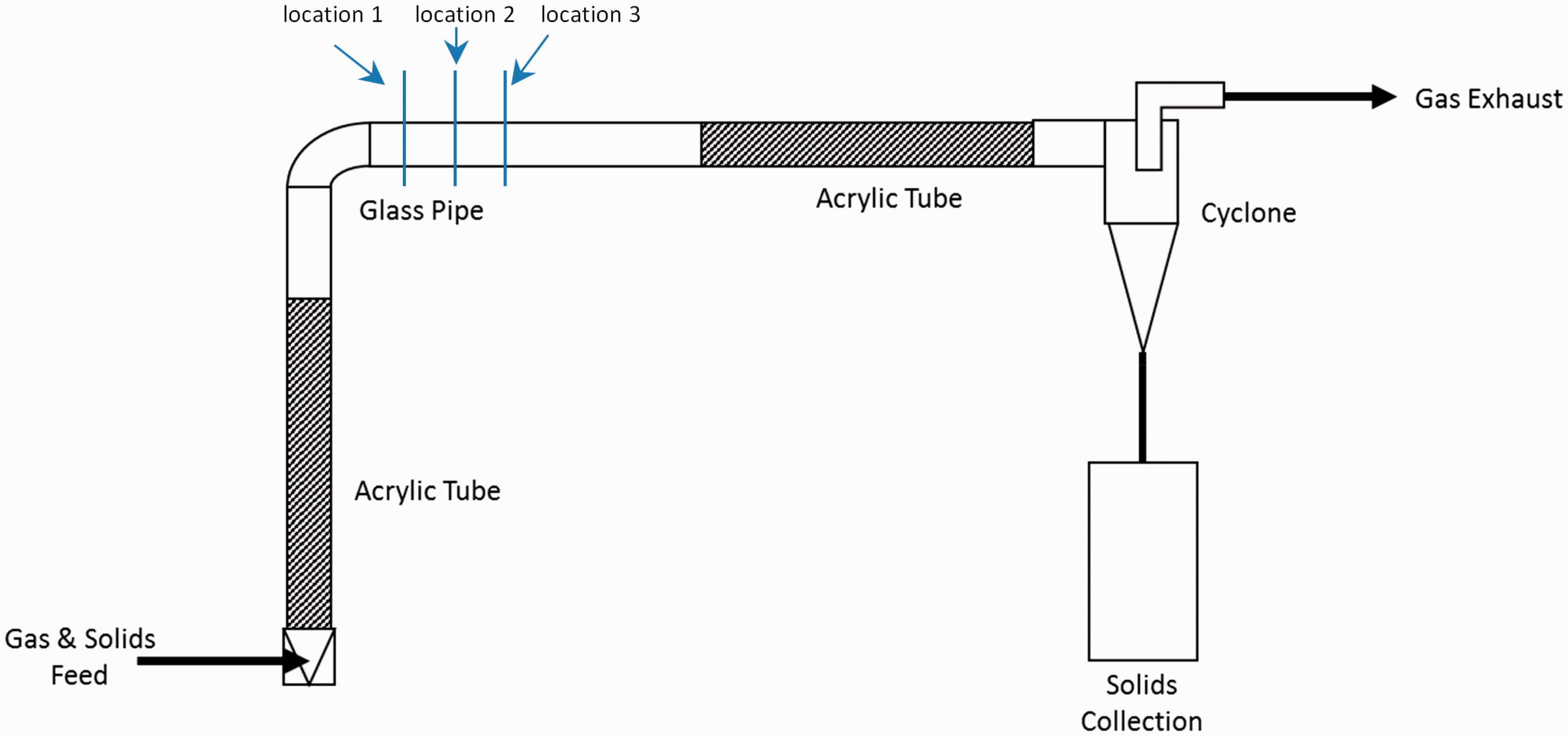

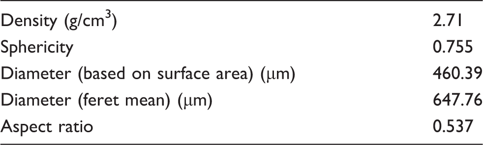
While the formation of ropes in pulverized coal-carrying pipe systems is of primary interest to this study, the tendency of fine (<100 µm) particle deposition and abrasion on the pipe walls prevents visual observation of the roping phenomena. Therefore, the solid material used in this study was ground flaxseed. The particle size distribution for these particles is given in Figure 2, and other material properties can be found in Table 1. 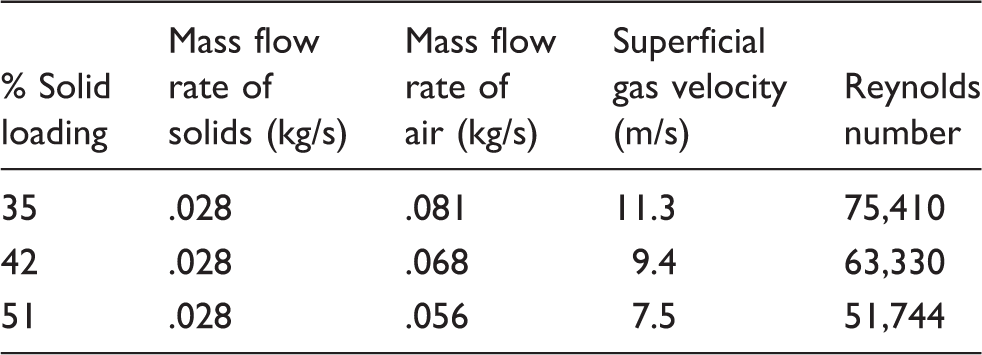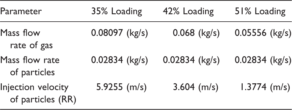The flaxseed was selected primarily because previous studies ⁵ showed it to be prone to roping at lower solid loadings, as well as non-abrasive so it would not scratch the glass. For this study, solid-to-air mass loadings of 35, 42 and 51% were obtained by maintaining a constant solid mass feed rate and varying the flow rate of air. Table 2 provides the exact flow rates used.

Figure 2.

Cumulative particle size and particle size density distributions for ground flaxseed particles (Courtesy of Mr. Jonathan Tucker, U.S. DOE NETL).

Table 1.

Flaxseed properties.

Density (g/cm3)	2.71
Sphericity	0.755
Diameter (based on surface area) (µm)	460.39
Diameter (feret mean) (µm)	647.76
Aspect ratio	0.537

Table 2.

Experimental test conditions.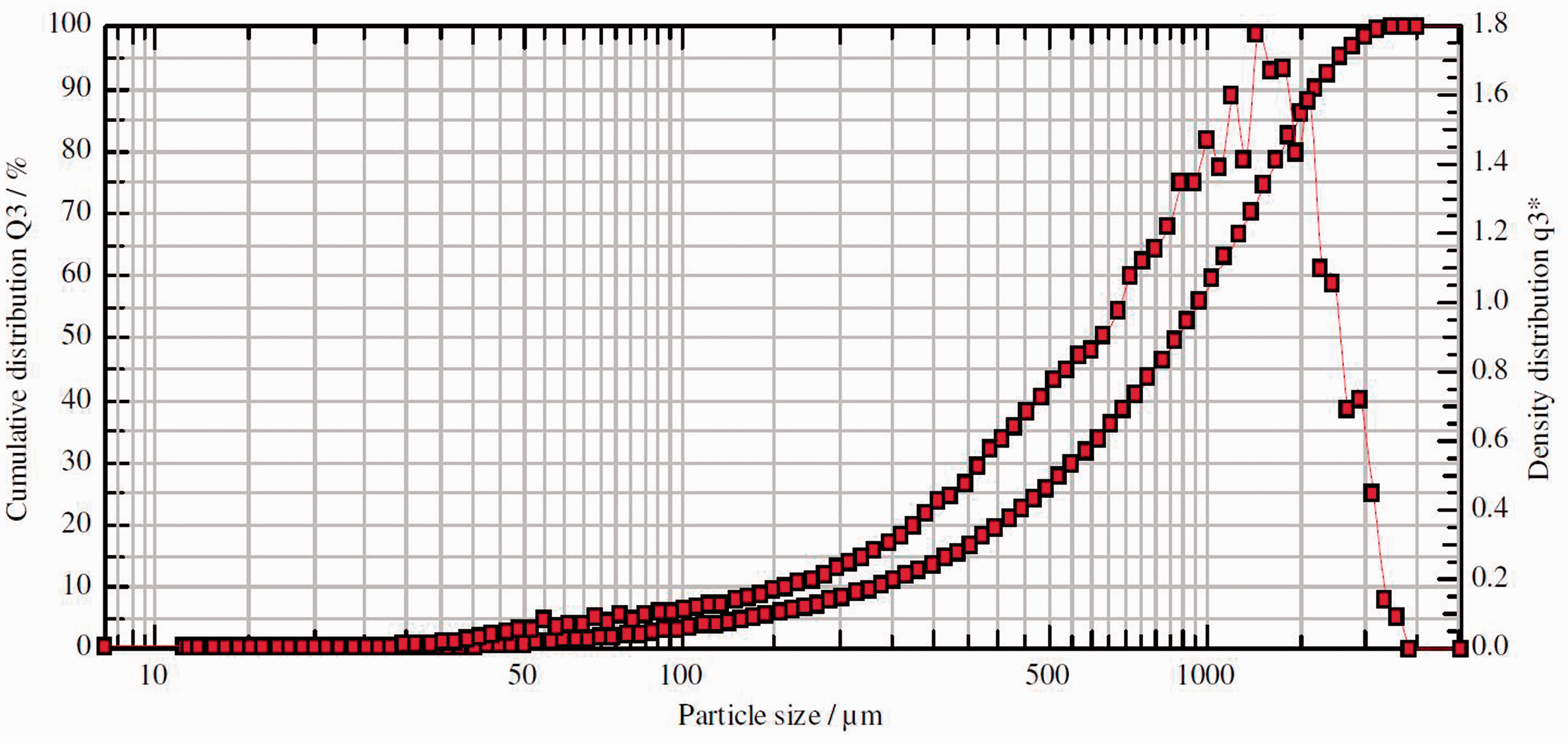

% Solid loading	Mass flow rate of solids (kg/s)	Mass flow rate of air (kg/s)	Superficial gas velocity (m/s)	Reynolds number
35	.028	.081	11.3	75,410
42	.028	.068	9.4	63,330
51	.028	.056	7.5	51,744

High-speed imaging of particle flow fields

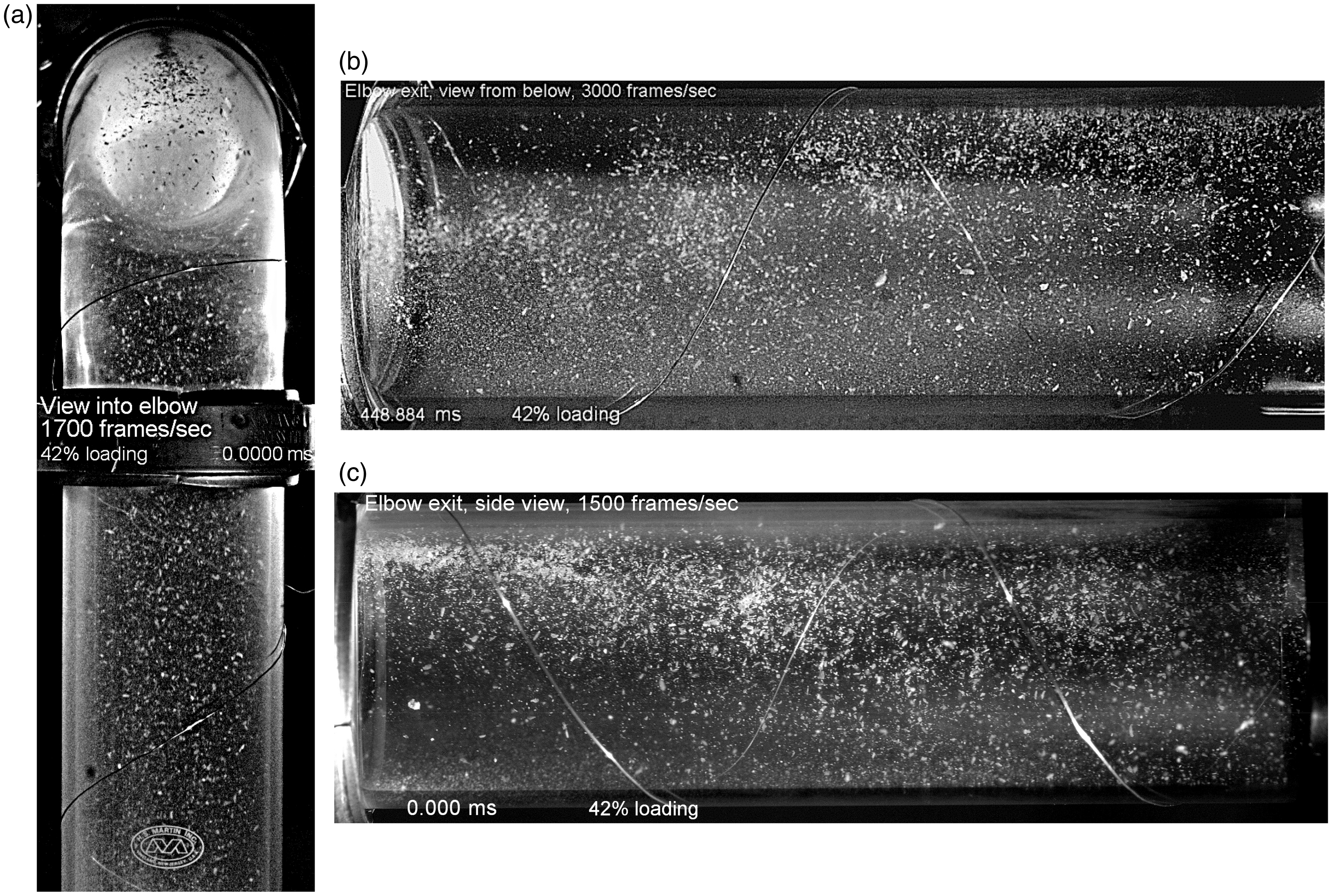
To capture the particle roping via high-speed video, three Vision Research high-speed cameras were set up with three orthogonal lines-of-view (perspectives). Figure 3 shows the orientation and lines-of-view of each high-speed camera. Camera 1, a Vision Research v12.1, had a line-of-view collinear with the pipe downstream of the elbow. Camera 2, a Vision Research v341, viewed the pipe downstream of the elbow exit from below, and Camera 3, also a Vision Research v341, viewed the pipe exit from a line-of-view from the side (normal to the plane of the pipe system). Cameras 2 and 3 were synchronized. Camera 1 was set to a resolution of 400 × 1280 pixels at 12-bit gray scale resolution at 1700 frames/s. Camera 2 was set at 1280 × 456 × 12-bit resolution at 3000 frames/s. Camera 3 was set at 2560 × 862 × 12-bit at 1500 frames/s. Figure 4 shows example images taken from each camera’s perspective. A detailed explanation of how the video recorded with these cameras was used for data analysis is presented in Calculation of particle concentration using high-speed video section.

Figure 3.

Camera perspectives for high-speed imaging of particle flow through a pipe elbow. This is a 2D plot for 3D setup of high-speed cameras. The pipe elbow has a ${90}^{\circ }$ angle, which is also labeled in the figure.

Figure 4.

Different views of cameras for high-speed imaging experiments. (a) Camera 1 view aligned with elbow exit. (b) Camera 2’s view of the elbow exit from below. (c) Camera 3’s view of the elbow exit from the side.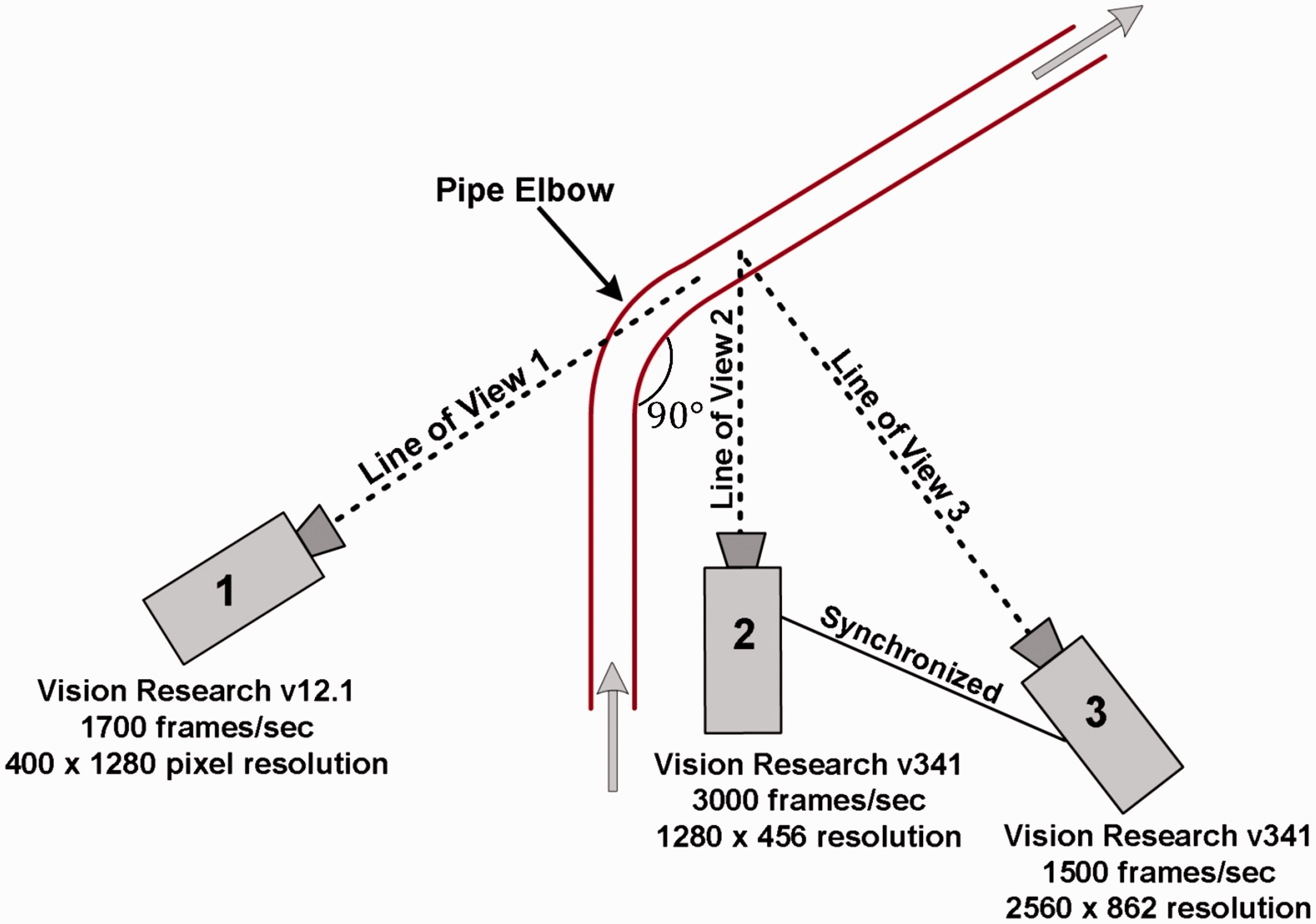

Simulations

For this study, a series of CFD simulations were created using the Ansys FLUENT software package. ⁶ For these simulations, two methods of turbulence modeling were used: the RANS model and large eddy simulation (LES) for turbulence modeling. These models are described in more detail in the following sections. It should be noted here, however, that it was not the intent of the authors to perform an exhaustive LES study of the roping phenomena. Instead, a very preliminary set of LES simulations were conducted and compared to the RANS results to see if the same general flow behaviors could be captured via RANS. A more thorough study via LES would have required a much finer grid resolution and processing resources.

Modeling Methodology

Governing equations

An Eulerian-Lagrangian approach is used for the gas–solid flow simulation. In this approach, the gas phase is treated as a continuum phase, and the solid particles are considered as a discrete phase. The gas phase is modeled on an Eulerian grid with the Navier-Stokes equations used as the governing equations. The motion of the solid particle phase is represented by the Lagrangian model approach, where the discrete particle phase is tracked by solving the equations of motion in a Lagrangian frame of reference. Equation (1) is the continuity equation and equation (2) is the momentum equation. Here, F is the external body force term which arises because of interaction with dispersed phase.

$$\begin{array}{c}\multicolumn{1}{c}{\nabla .(\overrightarrow{v})=0}\end{array}$$

(1)

$$\begin{array}{c}\multicolumn{1}{c}{\frac{\partial }{\partial t}(\rho \overrightarrow{v})+\nabla ·(\rho \overrightarrow{v}\overrightarrow{v})=-\nabla p+\nabla ·(\overline{\overline{\tau }})+\rho \overrightarrow{g}+\overrightarrow{F}}\end{array}$$

(2)

Here, F is the external body force term which arises because of interaction with dispersed phase.

The motion of solid particles is governed by Newton’s second law. By considering all the forces acting on the particle, the equation of motion can be written as ⁶

$$\begin{array}{c}\multicolumn{1}{c}{{\rho }_p\frac{d{\overrightarrow{U}}_p}{\mathit{dt}}={\overrightarrow{F}}_d+{\overrightarrow{F}}_b+{\overrightarrow{F}}_{\mathit{VM}}+{\overrightarrow{F}}_{\mathit{fp}}+{\overrightarrow{F}}_{\mathit{pp}}}\end{array}$$

(3)

where ${\overrightarrow{F}}_d$ , ${\overrightarrow{F}}_b$ , ${\overrightarrow{F}}_{\mathit{VM}}$ , ${\overrightarrow{F}}_{\mathit{fp}}$ , and ${\overrightarrow{F}}_{\mathit{pp}}$ represent the drag force, buoyancy force, virtual mass force, fluid–particle interaction, and particle–particle interaction, respectively. In present study, the particle–particle interactions are not considered. The drag force is defined as

$${\overrightarrow{F}}_d=F_D({\overrightarrow{u}}_g-{\overrightarrow{u}}_p)$$

(4)

with the coefficient

$$\begin{array}{c}\multicolumn{1}{c}{{\text{F}}_D=\frac{18\mu C_D\mathit{Re}}{d_p^{2}24}}\end{array}$$

(5)

and relative Reynolds number

$$R_e=\frac{\rho d_p|{\overrightarrow{u}}_g-{\overrightarrow{u}}_p|}{\mu }$$

(6)

where C_D is drag coefficient.

$$C_D=\frac{24}{\mathit{Re}}(1+b_1{\mathit{Re}}^{b_2})+\frac{b_3\mathit{Re}}{b_4+\mathit{Re}}$$

(7)

where

$$\begin{array}{c}\multicolumn{1}{c}{b_1=\text{exp}(2.3288-6.4581\varphi +2.4486{\varphi }^2)}\end{array}$$

$$\begin{array}{c}\multicolumn{1}{c}{b_2=0.0964+0.5565\varphi }\end{array}$$

$$\begin{array}{c}\multicolumn{1}{c}{b_3=\text{exp}(4.905-13.8944\varphi +18.4222{\varphi }^2-10.2599{\varphi }^3)}\end{array}$$

$$\begin{array}{c}\multicolumn{1}{c}{b_4=\text{exp}(1.4681+12.2584\varphi -20.7322{\varphi }^2+15.8855{\varphi }^3)}\end{array}$$

where ϕ is known as the shape factor. The shape factor used in these simulations is 0.755.

The discrete phase model (DPM) of Ansys Fluent is used for the trajectory of each individual particle.

Turbulence model

The effects of turbulence are critical in the modeling of gas–solid flows, especially for the roping phenomena inside the pipe bend. Here, we considered only two turbulence models, including RNG $k-\epsilon$ model^8,9 and LES model.^7–10 Other RANS models were also tested which did not show any appreciable difference in the simulation results. ⁵

The RNG $k-\epsilon$ model is a linear eddy viscosity model, and it is derived from renormalization group theory. Similar to other two-equation $k-\epsilon$ models, turbulent kinetic energy (k) and turbulent dissipation (ε) are solved from the two extra transport equations.^6,8,9 The details of governing equations can be found in Ansys, ⁶ as well as the meaning of terms involved in the equations. Here, we use the standard values of $C_{1\epsilon }$ and $C_{2\epsilon }$ , which are 1.42 and 1.68, respectively. $C_{\mu }$  = 0.0845.

The gas–solid flow within a pipe bend is also investigated using LES for the gas phase. Unlike direct numerical simulation (DNS) which resolves the eddies for all the length and time scales, LES only resolves the large eddies, which makes LES comparatively more efficient and less costly than DNS. The effects of the smaller, unresolved eddies on the resolved flow are included with the help of a sub-grid scale model.^10,12,13 The SGS model used in this study is Smagorinsky-Lilly model ⁶ with the eddy viscosity relation given by Ansys ⁶ and Smagorinsky. ¹⁰ The commonly used value 0.1 was used in our study for Smagorinsky constant, C_s.

Geometry and mesh

Figure 5 shows the sketch of the 3D pipe bend geometry. The inner diameter of the pipe is 3-in. (7.5 cm) (D). The computational models consist of a vertical pipe of five pipe diameters (5D), a horizontal pipe of 30 pipe diameters (30D) and a bend of radius 1.8 pipe diameters (1.8D). This curvature ratio, 1.8, is close to the commonly used ratio, 1.5, in the industry. ¹⁹ The hexahedral computational mesh was used in all the simulations. For the RANS simulations, a coarse mesh with 91,530 cells was used. For the LES simulations, a relatively finer mesh with 579,690 cells was used.

Figure 5.

Sketch of the 3D pipe bend used in the present study.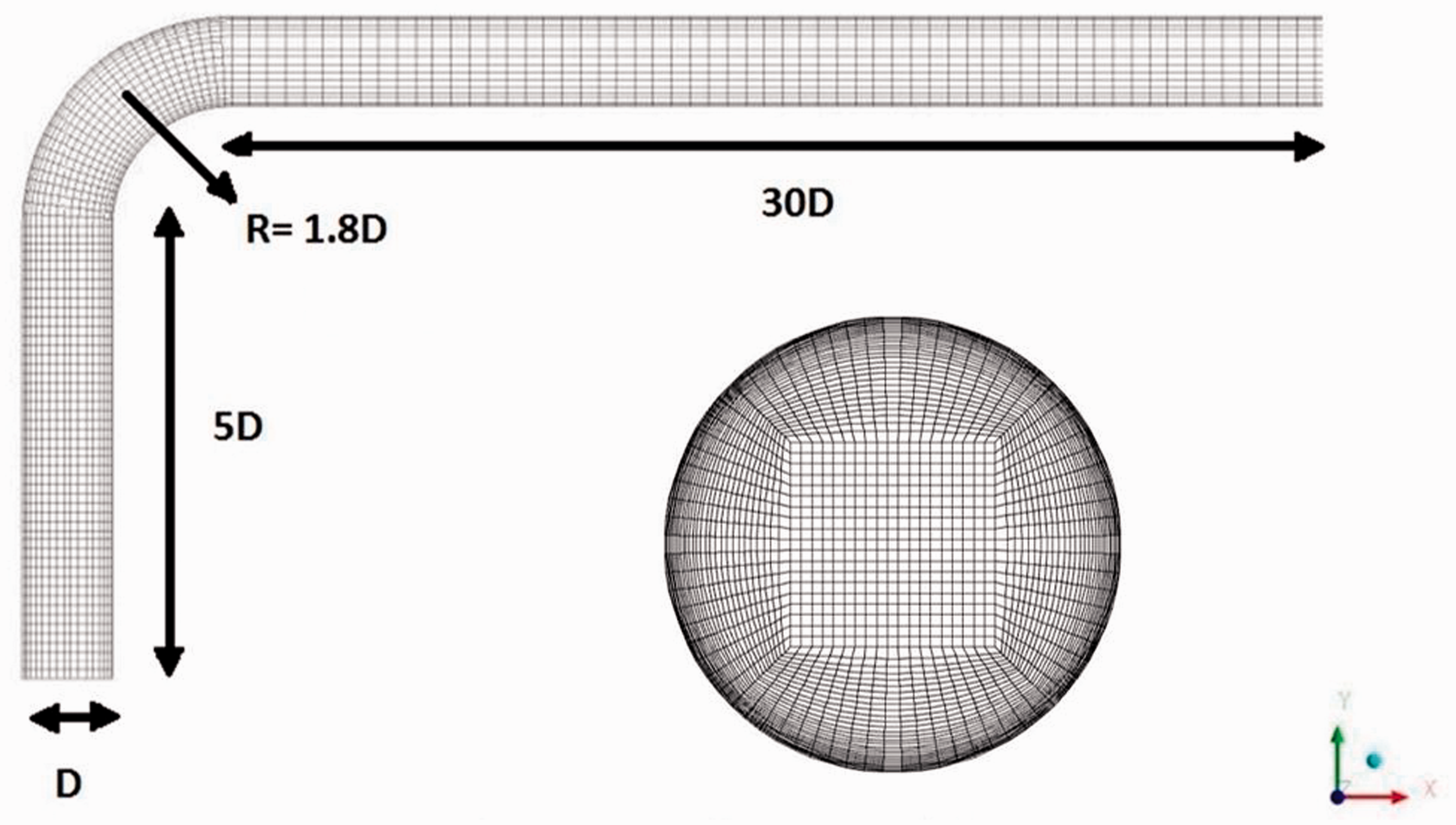

Results and discussion

For the current study, the high-speed video collected during the experimental testing was utilized in two ways for comparison to the simulation results. Firstly, representative still images were generated showing the particle flow field exiting the pipe elbow within approximately the first 12 in. of the horizontal pipe. These still images were then compared to the particle flow fields obtained from both RANS and LES simulations. Secondly, the high-speed data was analyzed to obtain average particle concentration profiles using the method described below. These resulting concentration profiles are likewise compared to similar profiles obtained at the same locations from the RANS and LES simulation results.

Calculation of particle concentration using high-speed video

Particle concentration was assumed to be proportional to the time-averaged brightness of particle images per unit area in the high-speed videos. Particle concentration fields are presented for the side view downstream of the elbow exit. Time averaging was done over 10,000 video frames which were recorded at 1500 frames per second, providing a total averaging time of 6.67 s.

To measure particle concentration using brightness in high-speed video, before time averaging, the effect of uneven illumination had to be removed and the particle images thresholded to render all particle images to the same brightness. The National Institutes of Health’s (NIH) ImageJ image analysis suite ¹⁴ was used for all steps in measuring particle concentration. A three-step process was used. The first step was to apply a bandpass Fast Fourier Transform (FFT) filter to remove spatial variations in brightness that were larger than the size of the particle images. The next step was to identify remaining background pixels (i.e. pixels with the same brightness in all video frames), then subtract the constant background brightness from each video frame. This step was accomplished using a plugin for ImageJ called Image Stack Merger. ¹⁵ The final step was to apply an Otsu threshold filter ¹⁶ so that all particle images were rendered to the same brightness. These steps resulted in a high-speed video at 8-bit grayscale resolution with all particles images at a brightness of 255 and all background pixels at a brightness of 0. Figure 6(a) shows a frame from a high-speed video of the flow field exiting the pipe elbow before the image processing steps were applied. Figure 6(b) shows the same video frame after a high-pass FFT was applied with a filter cutoff set at 35 pixels (the largest particle images were around 25 pixels in diameter). Figure 6(c) shows results after the background as subtracted using the Image Stack Merger plugin. Figure 6(d) shows the result after applying an Otsu thresholding filter.

Figure 6.

Analysis procedures for images taken by high-speed cameras. (a) Video frame from original high speed video showing particle flow field exiting the pipe elbow. (b) Figure (a) after a bandpass FFT was applied with a cutoff set at 30 pixels. (c) Figure (a) after subtracting the background image (Figure 3). (d) Results after applying an Otsu threshold filter. All particle images are of the same brightness.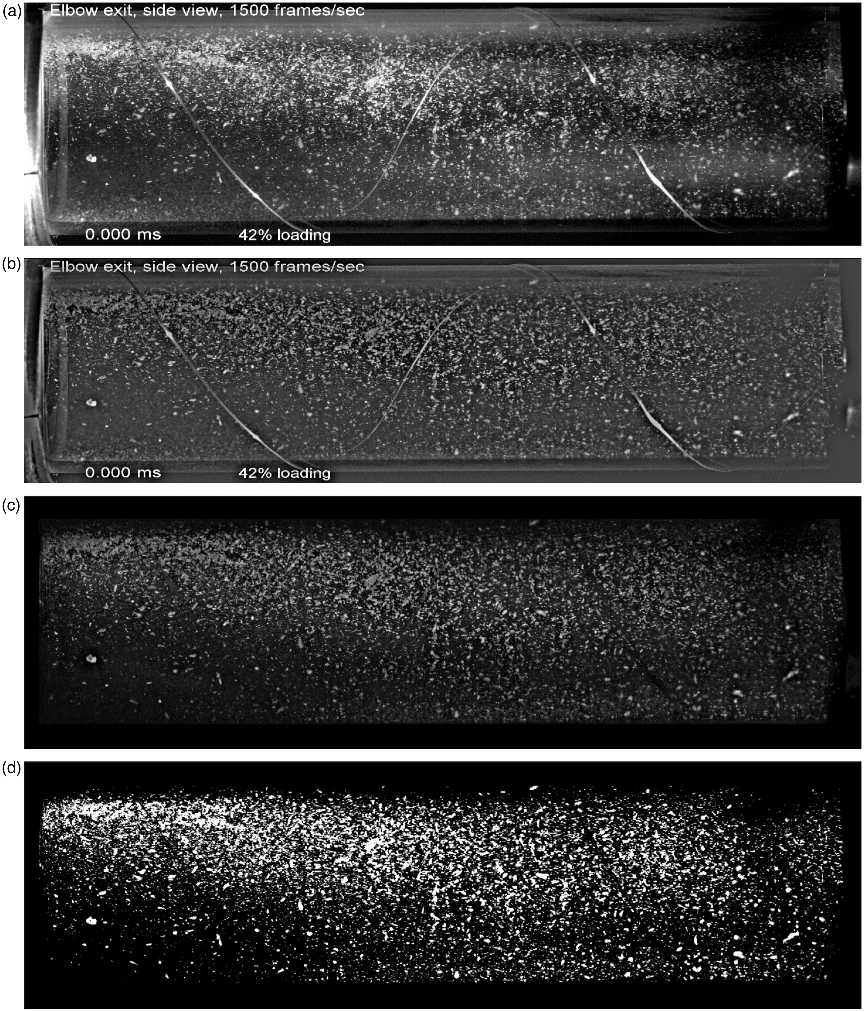

The concentration at any point in the video frame is normalized with the maximum concentration (i.e. the maximum brightness), which occurs in the particle “rope” when it exits the elbow at the upstream top of the elbow exit. Figure 7 shows the location of the maximum brightness. The pixels of the time-averaged frames were multiplied by a factor to set the maximum brightness to a level of 255. All concentration data are normalized with the maximum brightness value; therefore, all concentration data have a range from 0 to 1. It should be noted that the absolute value of particle concentration at the point of maximum brightness is not known. Therefore, the measured concentration is not absolute, but rather relative to the maximum for each flow condition.

Figure 7.

Location of maximum brightness/concentration.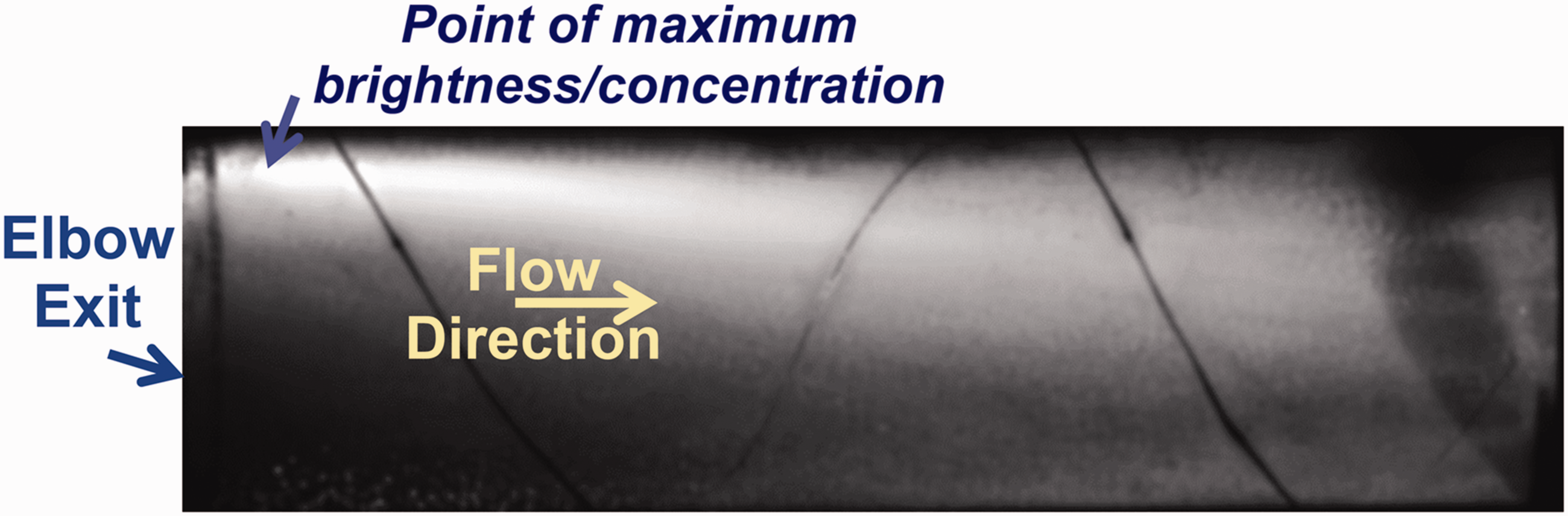

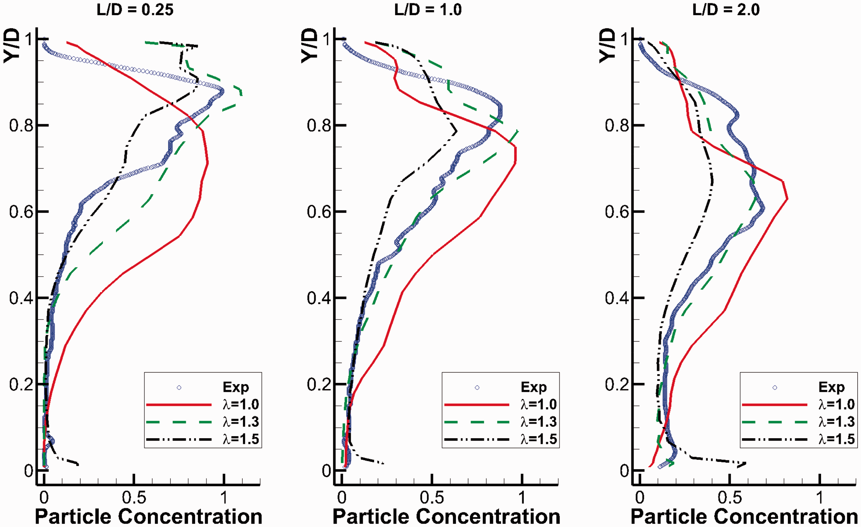
We calculated the particle concentration profiles at numerous locations. Here, we select three locations downstream of the elbow exit (monitor points 1, 2, and 3) where the wires wrapped around the pipe bend (for static charge grounding) can be avoided. These three selected locations are L/D = 0.25, 1.0, and 2.0, respectively, as shown in Figure 8 where L is measured from the inlet to the horizontal pipe. The measured particle concentration profiles at these locations are shown as radial profiles in Figure 9.

Figure 8.

Locations of radial profile measurements downstream of elbow exit.

Figure 9.

Particle concentration profiles calculated from high-speed videos via image processing scheme for three loadings: 35%, 42%, and 51%. (a) Monitor point 1, (b) monitor point 2, (c) monitor point 3.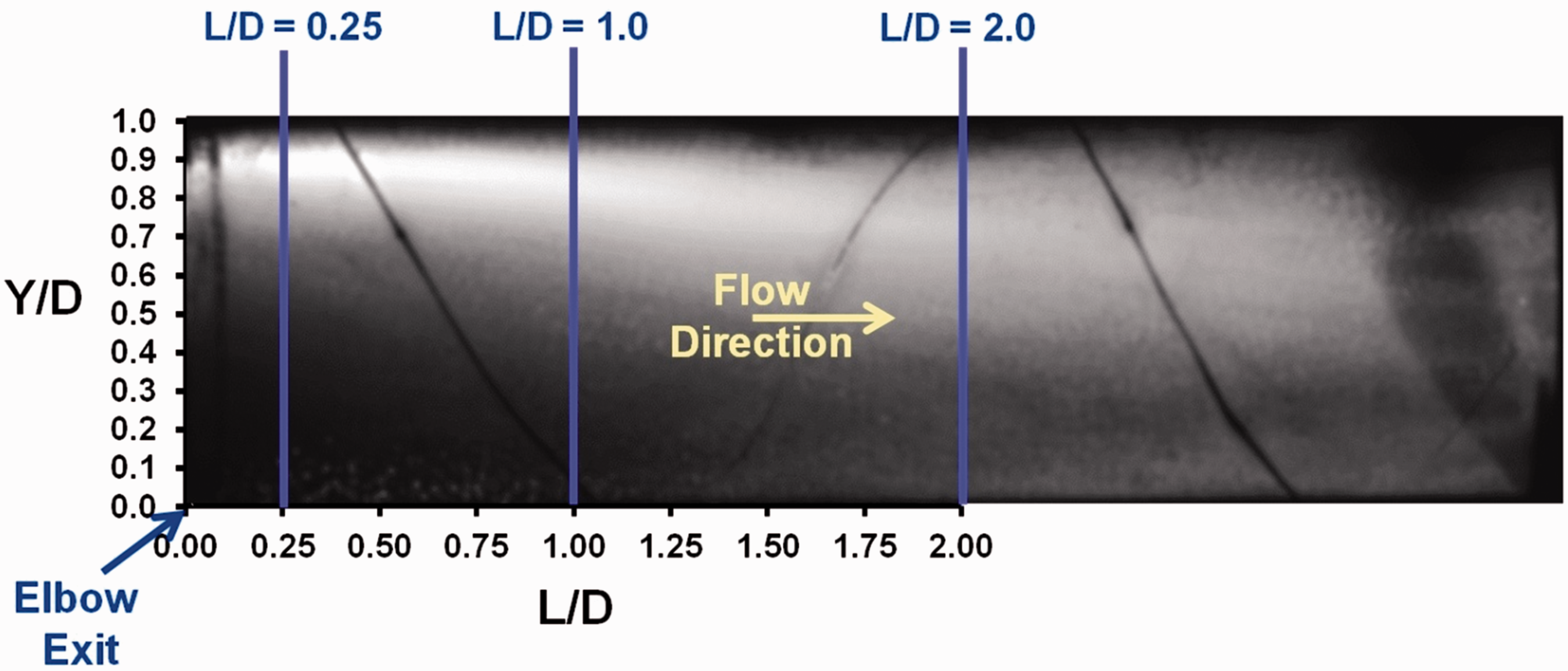

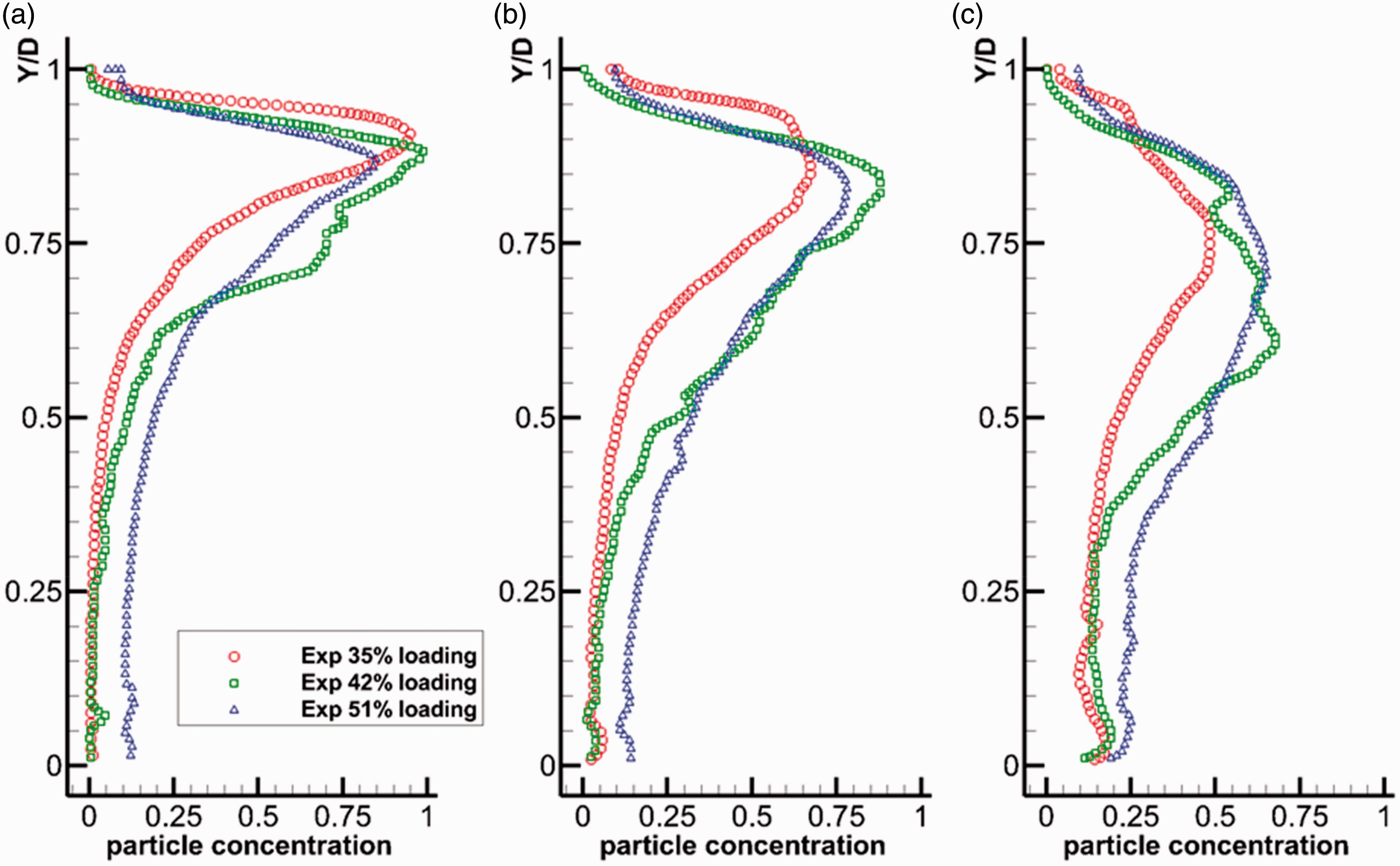
The results presented in Figure 9 show that, as the particles exit the elbow, they are initially concentrated near the top of the pipe. As the particles progress further down the horizontal pipe away from the elbow, they become more diffuse and spread out over a larger portion of the pipe radius. Interestingly, the results suggest that the 42% loading case seems to take longer to disperse than does the higher 51% loading case. For the case of 42% loading, the particle roping can be clearly identified.

CFD results and discussion

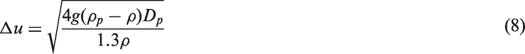
In addition to experiments, numerical simulations were performed using Ansys Fluent CFD package to investigate the gas–solid flow inside a pipe bend. We investigated the gas–solid flow inside a pipe bend with the aforementioned RANS and LES turbulence models. The slip velocities were calculated based on mean particle size using the Rosin-Rammler (RR) distribution function. Slip velocity calculation is given by

$$\begin{array}{c}\multicolumn{1}{c}{\Delta u=\sqrt{\frac{4g({\rho }_p-\rho )D_p}{1.3\rho }}}\end{array}$$

(8)

where g is acceleration due to gravity, ${\rho }_p$ is density of particles, ρ is density of gas and D_p is particle diameter.

The shape factor was set to 0.755. The particle images were recorded in a similar manner to the images obtained with the high-speed video, and similar image processing was applied to particle concentration profiles.

Mesh sensitivity

A mesh sensitivity study was performed to assess the magnitude of discretization errors with the intention to show that they will not dominate the physics of the problem. Three meshes were generated, namely (i) coarse mesh with 9879 cells, (ii) medium mesh with 91,530 cells and (iii) fine mesh with 684,456 cells. The finest mesh had some nodes where y₂_plus (the y-plus value at the cell center nearest to the wall) was <15. This was avoided by deleting several nodes near the wall region. The resulting y₂_plus values for the three meshes were 42, 18, and 34, respectively. These values are considered appropriate for application of standard-wall functions, as is the case in the present simulations. The concentration profiles were observed at vertical lines at the center, and a distance of 0.25 D to the left and to the right from the center. Figure 10 shows the particle concentration profiles at a location of 0.25 diameters (D) axial distance from the bend exit for all the three meshes along the three vertical lines mentioned above. Although it is hard to claim that grid convergence is achieved, it can be said that the conclusions reached using the simulations from medium mesh will not change significantly if much finer meshes were used in conjunction with the standard wall functions.

Figure 10.

Grid convergence behavior of the predicted concentration profiles.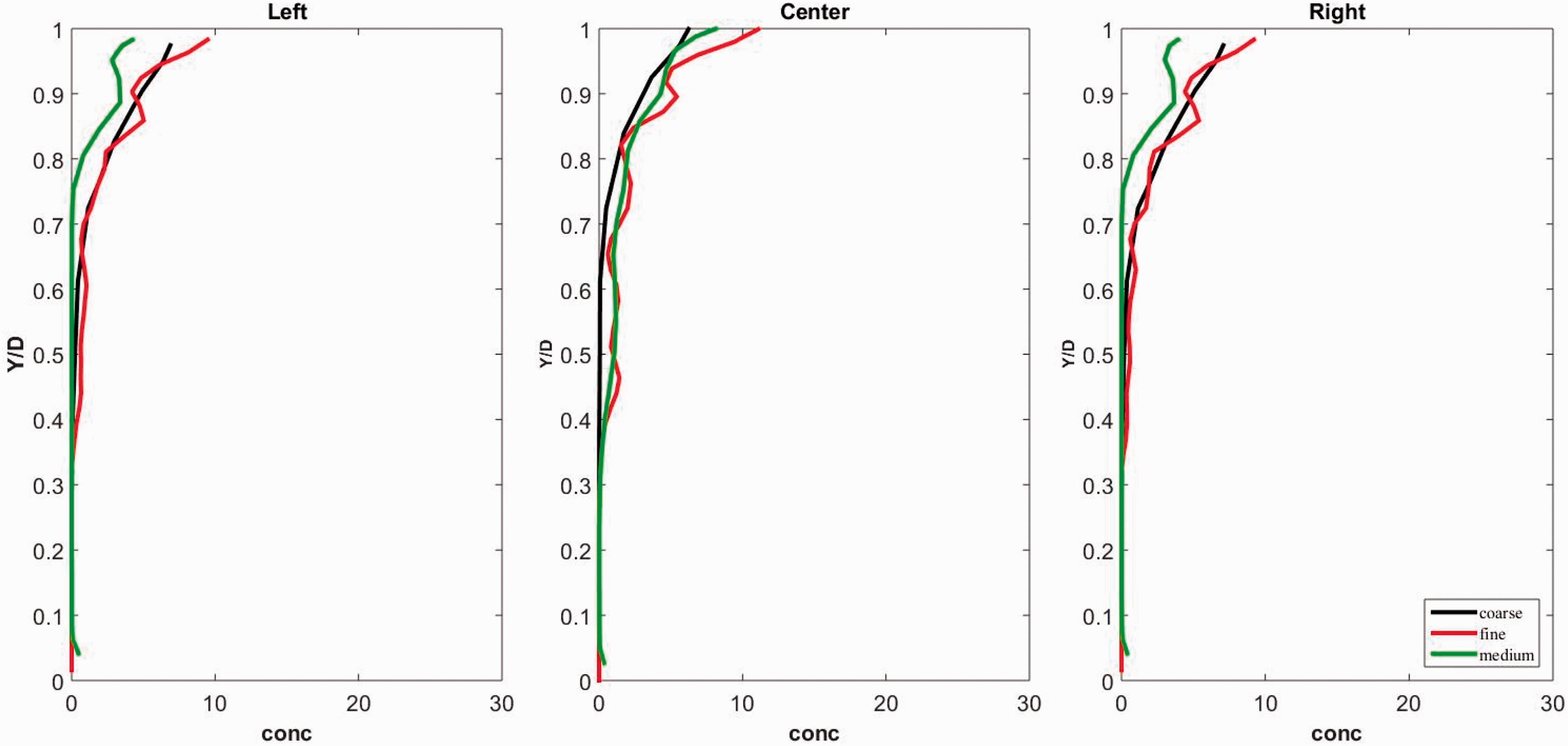

Simulation details

The simulated cases in the present study are summarized in Table 3. Simulations were performed for solid–gas loadings (mass flow rate of solids/total mass flow rate) of 35%, 42%, and 51%. The simulation details of the different loading conditions are listed in Table 4. The details of the RANS and LES simulations are shown in Table 5. In all cases, the solid material is ground flaxseed with a density of 2710 kg/m³. The boundary conditions for inlet and outlet are velocity inlet and pressure outlet. A particle injection file with random distribution has been specified at the inlet. For the walls, the reflect boundary condition has been used for the particles with constant values of tangential and normal coefficients of restitution. The pressure–velocity coupling used is SIMPLE. The spatial discretization for pressure is PRESTO. Bounded central differencing scheme has been used in the simulations. This scheme is well suited for LES and prevents any unnecessary fluctuations in solution fields. Second-order implicit transient formulation has been used in the simulations. The gas–solid flow behavior through a pipe bend is a highly unsteady phenomenon. Hence, transient simulations with unsteady particle tracking have been performed. Also in order to closely replicate the experimental conditions and also to generate particle trajectory videos for comparison with high speed experimental videos, the above-mentioned strategy has been adopted. For inlet boundary conditions, a representative Gaussian distribution of particles is specified in the following case studies. This is very like the realistic cases in the experiments.

Table 3.

Summary of simulated cases about gas-solid flow in present study.

Case no.	Loading condition, %	Diameter distribution scheme	Turbulence model
1	35	RR (40–2183 mic)	RNG $k-\epsilon$
2	42	RR (40–2183 mic)	RNG $k-\epsilon$
3	51	RR (40–2183 mic)	RNG $k-\epsilon$
4	35	RR (40–2183 mic)	LES
5	42	RR (40–2183 mic)	LES
6	51	RR (40–2183 mic)	LES

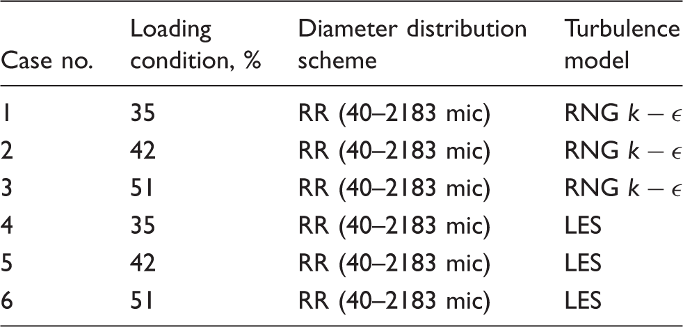
LES: large eddy simulation; mic: micron (unit of particle diameter).

Table 4.

Simulation details of different loading conditions.

Parameter	35% Loading	42% Loading	51% Loading
Mass flow rate of gas	0.08097 (kg/s)	0.068 (kg/s)	0.05556 (kg/s)
Mass flow rate of particles	0.02834 (kg/s)	0.02834 (kg/s)	0.02834 (kg/s)
Injection velocity of particles (RR)	5.9255 (m/s)	3.604 (m/s)	1.3774 (m/s)

Table 5.

Simulation details of RANS and LES simulations.

Parameter	RANS	LES
Time step size	0.001	0.0001
Transient formulation	First order implicit	Second order implicit
Spatial discretization – momentum	Second order upwind	Bounded central differencing

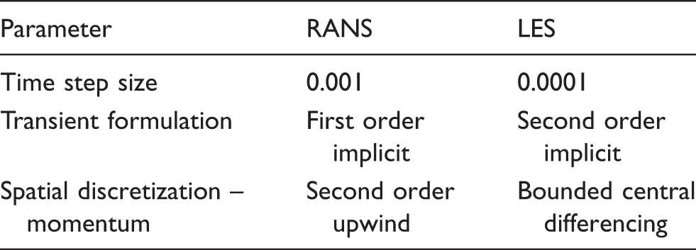
LES: large eddy simulation; RANS: Reynolds Averaged Navier-Stokes.

Simulation results

Gas flow predictions in the pipe bend

In our simulations, the pure flow field was simulated for long enough time before injecting the solid for roping study. Figure 11 shows the flow field obtained from LES simulations. The results show flow separation at the inner section of the elbow. Although different turbulence models were used in the literature, similar observations and conclusions as ours were obtained.^18–20 It was observed that the mean velocity is small near the inner section of elbow which may cause a reverse flow in some situations. Therefore, we conclude that our results match the literature qualitatively, and our simulation is able to capture the primary flow phenomena in pipe bends adequately.

Figure 11.

Flow field within pipe bend before injecting the solid. The location of selected cross-sections are labeled, which is the same as in Figure 8.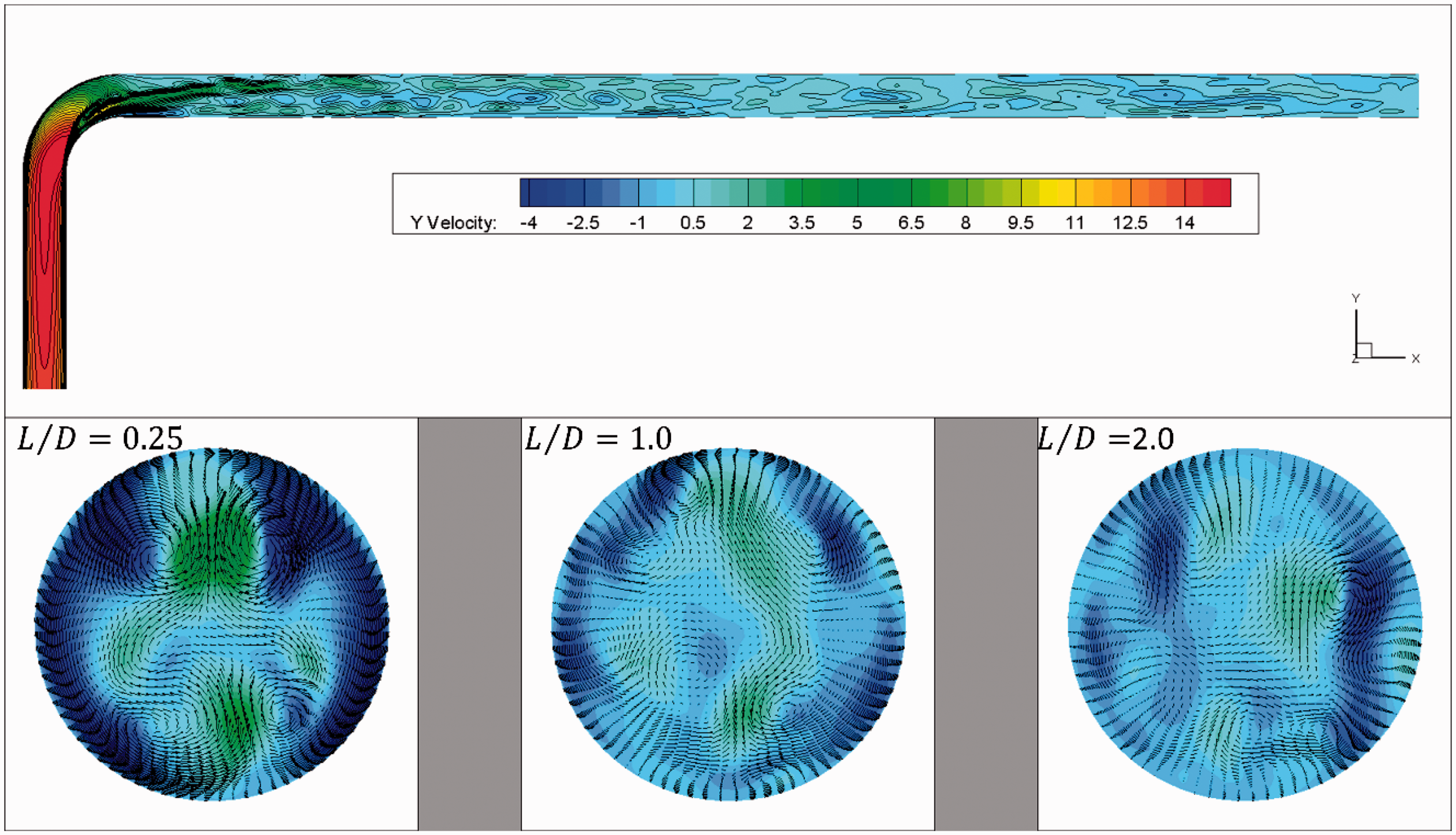

Comparison of experiments and simulations

In this section, results from experiments, RANS simulations, and LES simulations are compared with each other. For each simulated case, the particle history data were exported and visualized. Figure 12 compares the particle visualization results from both the RANS and LES simulations to the experimental data for the elbow and horizontal pipe side view, as well as a view of the horizontal pipe section just downstream of the elbow exit. It is seen that, while there are variations between the LES and RANS results, both can predict the general trends of the rope formation seen during the experiments, thus confirming that the simulations account for the correct flow physics as observed in experiments, if the value used for coefficient of restitution is accurate.

Figure 12.

The comparison between experiments and simulations for 42% loading.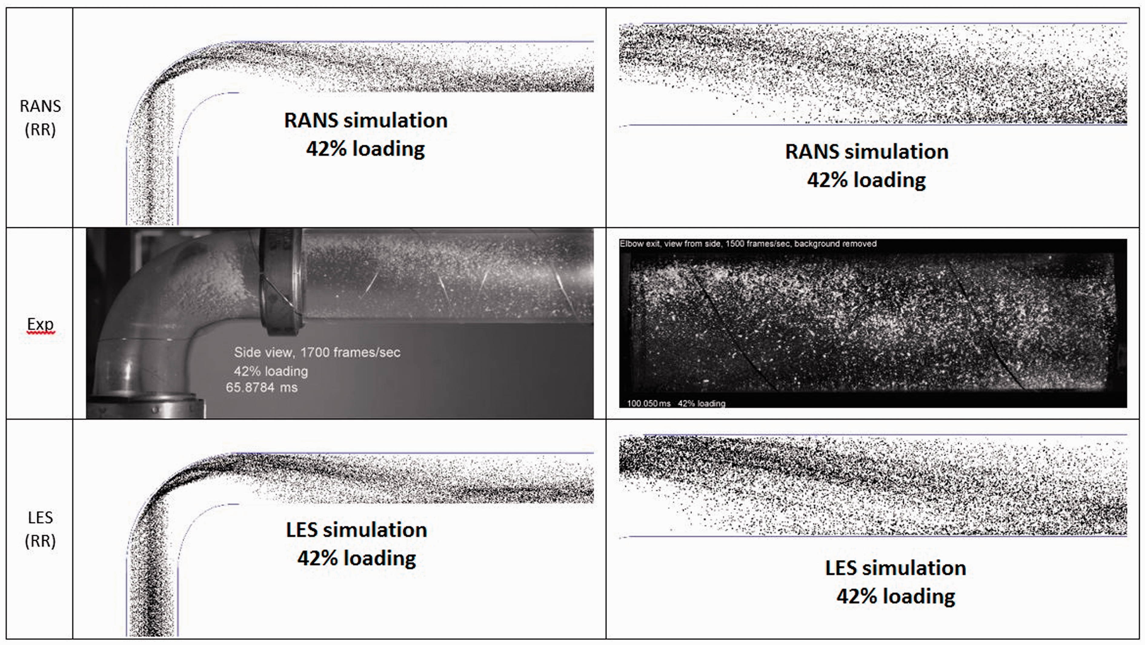

Additionally, further confirmation of this can be seen in the quantitative comparison of solid concentration profiles for solid loadings of 35, 42 and 51%, as shown in Figures 13. In these figures, the RANS and LES simulations provide roughly similar solid concentration profiles that match well with those obtained via analysis if the high-speed video.

Figure 13.

Particle concentration profiles from experiments and simulations for (a) 35%, (b) 42%, and (c) 51% loading condition.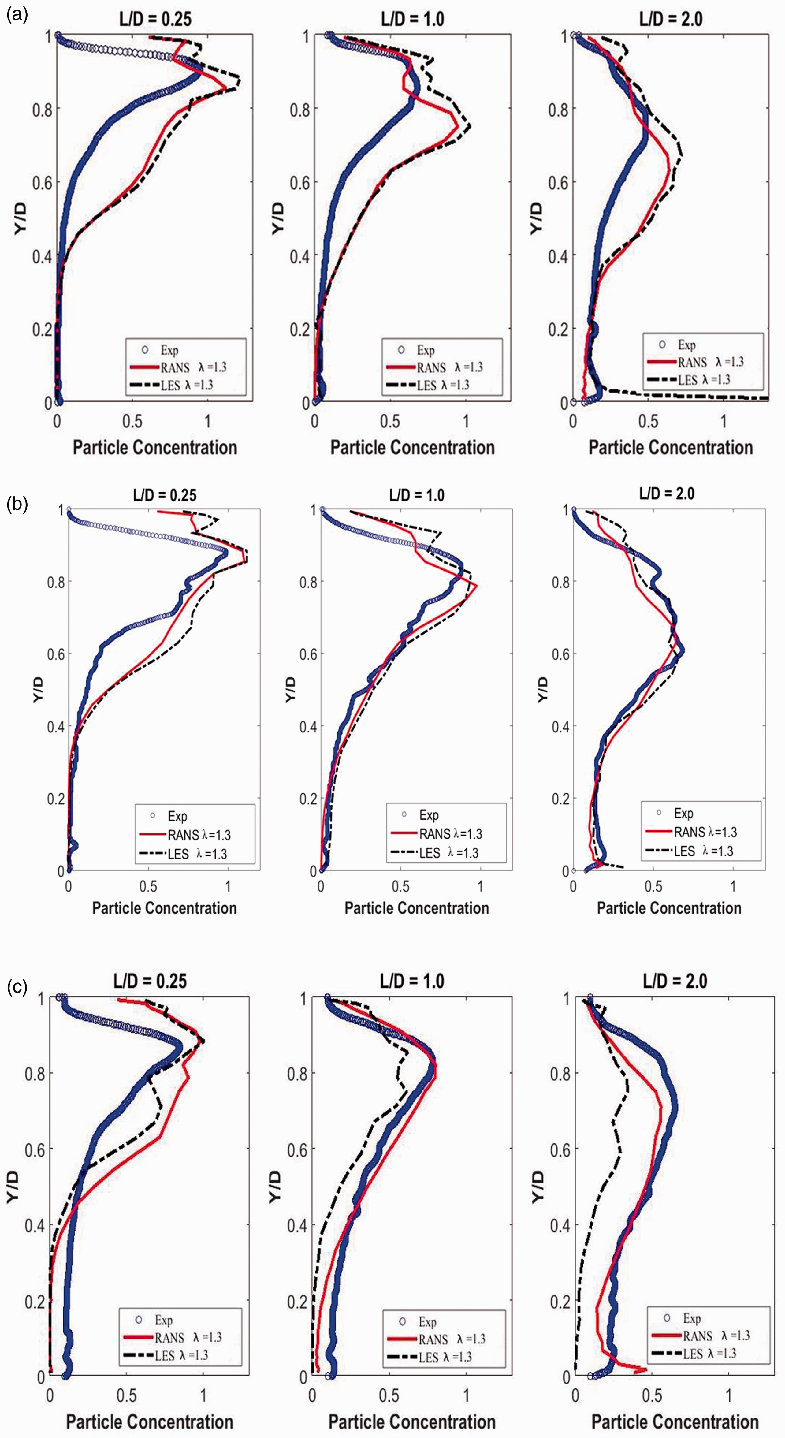

Further investigation of roping mechanism

In this section, we would like to investigate the effects of restitution coefficient on the roping within pipe bend. The relation between vorticity and formation of roping is also studied by comparing the results from RANS and LES turbulence model. Analysis of these effects on the flow field and local solid concentration profiles will help us better understand the mechanism of roping.

Restitution coefficients

The restitution coefficient determines the reflection angle and momentum exchange/loss when solid particles collide with the wall, especially the elbow section. Aspherical particle shape produces a variation in restitution coefficient, with a time-averaged mean value and variation around the mean. 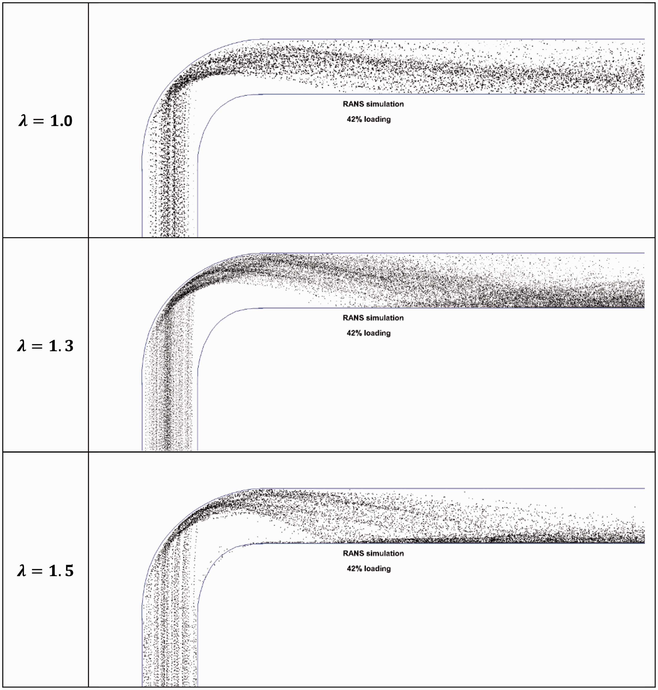¹⁷ Although experimental measurement of restitution coefficient for aspherical particles is difficult, ¹⁷ it is a required input in CFD models. The effects of restitution coefficient are also investigated in the present study. RANS simulations were performed for 42% loading cases with various values of λ, defined in Figure 14. Figure 15 shows the effects of λ on the calculated gas–solid flow. It can be observed that the particle concentration profiles are very sensitive to restitution coefficients. This conclusion can also be confirmed by particle visualization shown in Figure 16. The results show that without having an accurate value for λ, the roping phenomena cannot be predicted. Thus, we employed the visualization experiments to determine an approximate λ value, 1.3, for the currently used solid material.

Figure 14.

Definition of parameter $\underset{¯}{\lambda }$ in the study of restitution coefficients.

Figure 15.

Particle concentration profiles from experiments and the RANS simulations for 42% loading condition with various values of $\underset{¯}{\lambda }$ .

Figure 16.

Particle visualization figures from the side view for RANS simulations for 42% loading condition with various values of 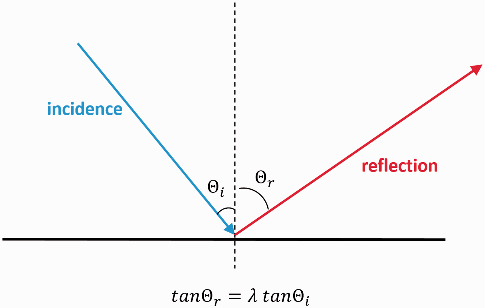$\underset{¯}{\lambda }$ .

Further comparisons between RANS and LES

Figure 17 shows particle concentration profiles for the pipe cross-section and different L/D locations downstream of the elbow exit for both RANS and LES simulations for the 42% loading case. It is seen from the figure that, while LES provides better resolution and the ability to predict large eddy structures, the same general trends are shown in both sets of results with respect to the distribution of solids within the pipe cross-section.

Figure 17.

Particle concentration contour at different cross sections from RANS (top) and LES (bottom) simulations for 42% loading condition.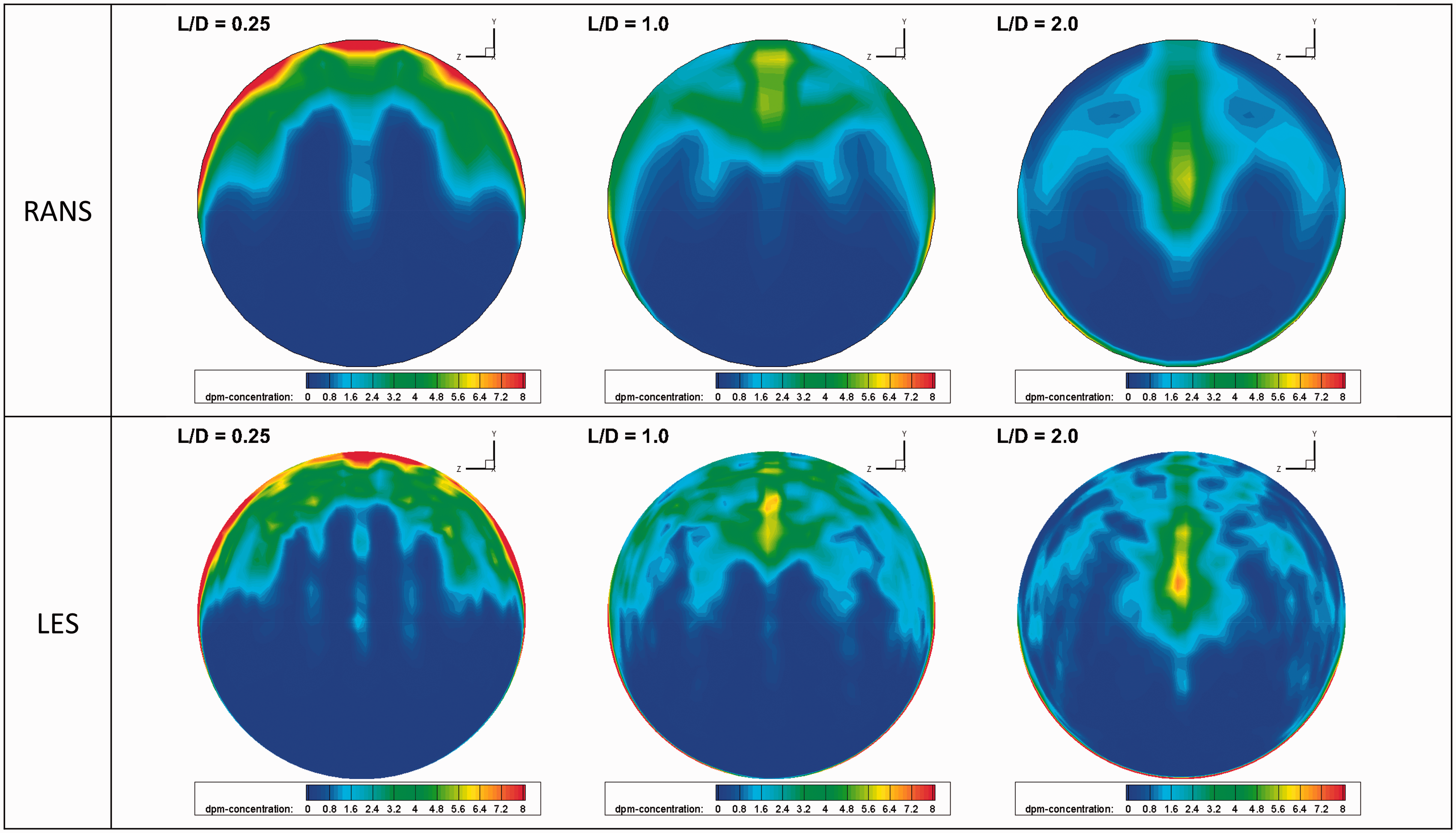

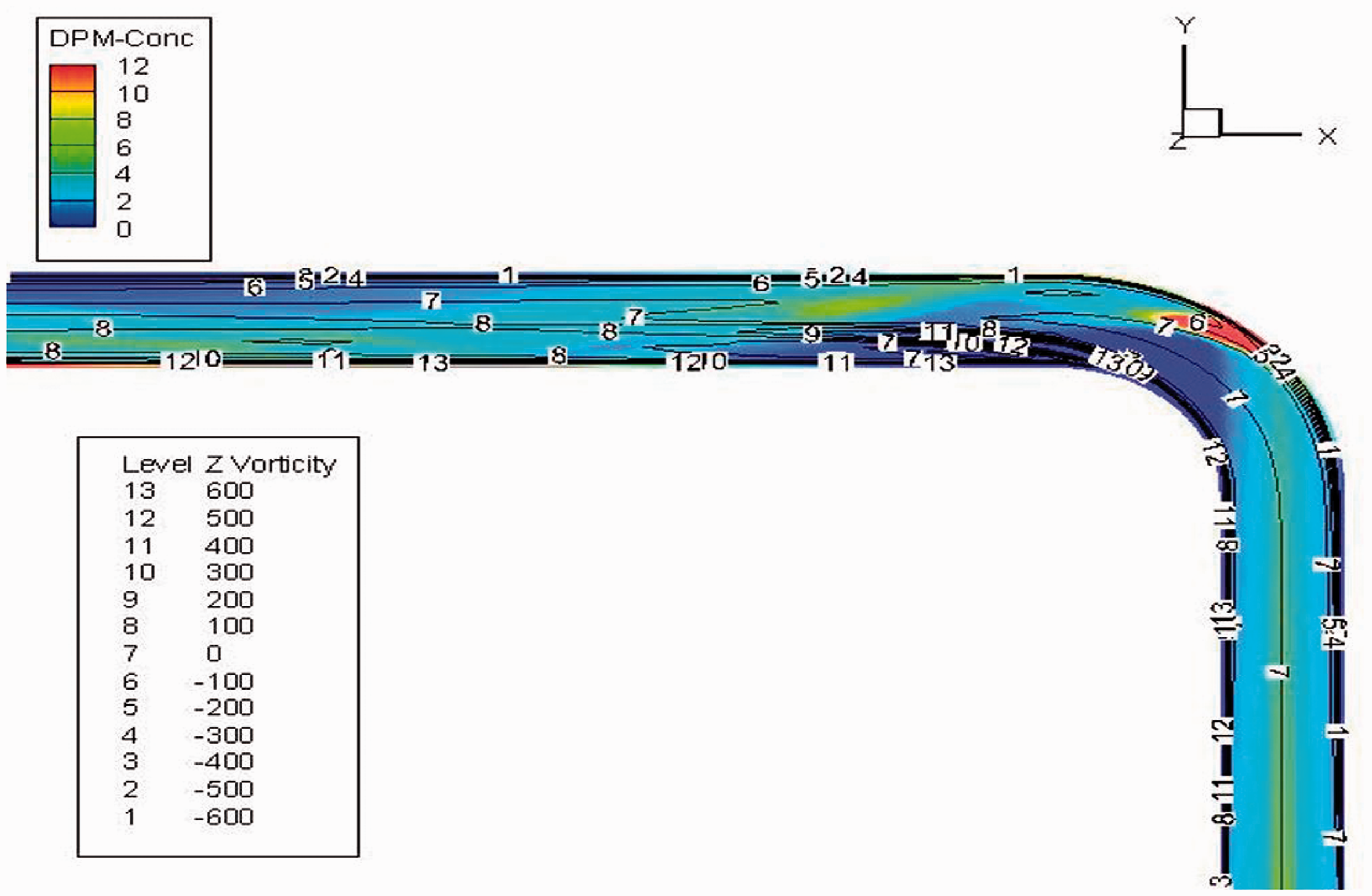
Effect of vorticity on solid concentrations

Figures 18 and 19 show solid concentrations superimposed by iso surfaces of x- and z-direction gas vorticity for both pipe cross-sections and elbow/pipe side views, respectively. It can be observed that a close correlation exists between the concentration of particles and the vorticity. The regions where particles are concentrated are bounded by vortices of same magnitude (100) both in clockwise and counter-clockwise direction (indicated by lines 6 and 8 in Figure 18). It can also be observed that, at the exact location where particles are concentrated, the vorticity is zero. From this, it is concluded that the rope phenomena and vorticity within the gas flow are strongly inter-related.

Figure 18.

Solid concentration profiles with x-direction vorticity contours superimposed at different pipe cross sections for the 42% loading case.

Figure 19.

Side view showing solid concentrations superimposed with Z-direction vorticity for the 42% loading case.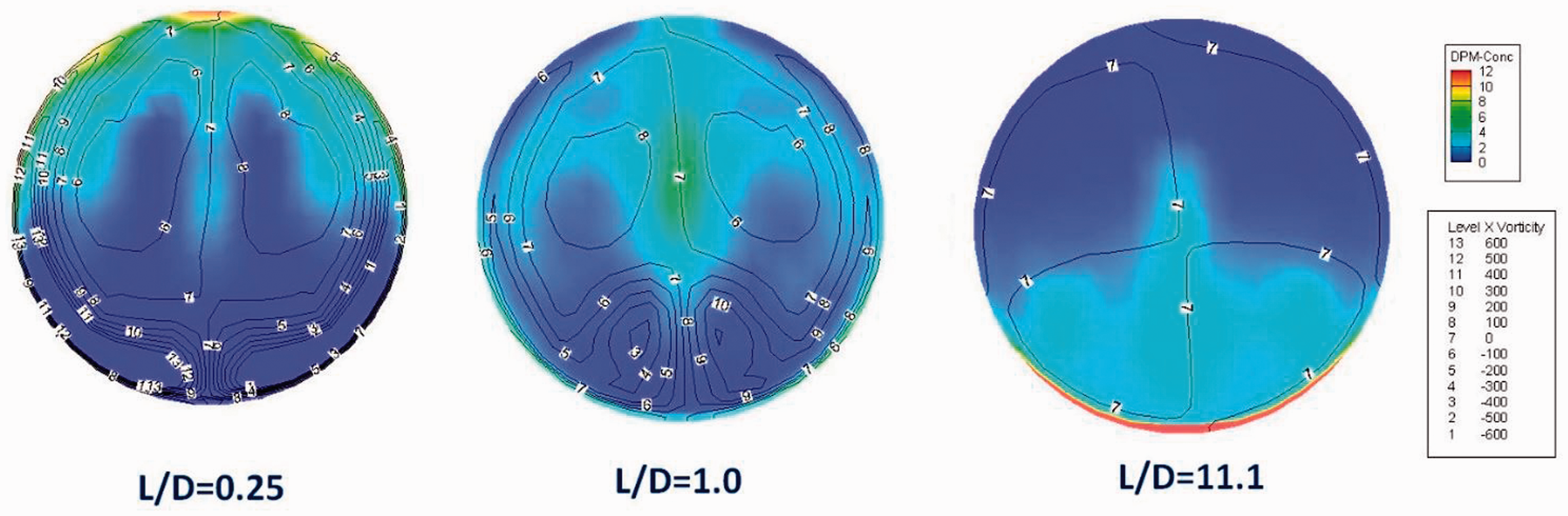

Conclusions

A study was conducted in which CFD simulations of solids-laden air flow through a 90° vertical to horizontal elbow were compared to experimental data obtained via analysis of high-speed video. Simulations using both RANS and LES turbulence models were analyzed to obtain solid concentration profiles that were then compared to the experimental data. Upon comparison, it was determined that both RANS and LES models could accurately predict the formation of particle roping. However, it was also determined that the accuracy of the simulation results depended greatly upon appropriate selection of the value of the coefficient of restitution. Because of these results, it can be concluded that the less computationally intensive RANS method is sufficient to capture the physics involved in rope formation within pipe flows, thus negating the need for more resource intensive LES simulations, as suggested by previous authors who have explored the simulation of particle roping.^2–5

Finally, it was observed from the simulation results that there is a direct link between gas vorticity and solid concentration. It was shown that areas of high solid concentration were bounded by regions of high vorticity, but also that vorticity is zero in the high solid concentration regions.