Sage Journals: Discover world-class research

Abstract

A growing interest for the design of structures to sustain blast-induced loads has been observed in recent years as a result of the worldwide rise of terrorist bombing attacks. The blast loading is usually characterized by a sudden increase in the pressure followed by an exponential decay. The parameters of this pressure pulse are essential for design and can be found in various blast design manuals available in the open literature. One of the most widely used sources is a technical report by Kingery–Bulmash, which provides values for many blast parameters in diagrams and polynomial form. However, it does not include an equation for calculating the blast wave decay coefficient, necessary for constructing the pressure–time history of an explosion at a certain point. In this study, a review of the technical literature that contains expressions for the blast pressure decay coefficient is performed, and relevant comparisons have been made. New equations describing the decay coefficient of the Friedlander equation for both incident and reflected cases for free-air and surface bursts are proposed. These equations express the decay coefficient in terms of the scaled distance and are not valid for close-in detonations. They are entirely based on the Kingery–Bulmash data, and their accuracy is satisfactorily checked against new experimental results and their trends assessed through a sensitivity analysis. Accordingly, the positive phase of the pressure–time curve at a point can be reliably and efficiently generated.

Keywords

Decay coefficient explosion modeling Friedlander equation Kingery–Bulmash

Introduction

Explosions due to terrorist attacks, as a result of the worldwide rise of terrorism, have in the last decades become a serious problem, especially because such attacks may result in a large number of fatalities. These fatalities can be the outcome of both the direct exposure to the blast wave from the explosion and of structural failures that could lead to progressive collapse of buildings and other structures. Famous examples of such actions are the bombing attacks against the A. P. Murrah governmental building at Oklahoma City, OK, USA, in 1995 and the simultaneous bombing of the US embassies at the cities of Dar es Salaam, Tanzania, and Nairobi, Kenya in 1998. The speculation that civilian and federal buildings could serve as possible targets of terrorist groups became a certainty after the attack that led to the collapse of the World Trade Center on 11 September 2001.

An explosion lasts only some milliseconds and is characterized by the release of hot gases that expand through the air occupying all available space, leading to the creation of the blast wave. Each blast wave is typically characterized by a set of parameters that can be calculated based on various technical manuals that have been mainly developed by the military community. The most reliable and widely used references appear to be some US military publications, such as the Army Technical Manual (Department of the Army, 1990) or its more recent version known as Unified Facilities Criteria (2008), and a technical report by Kingery and Bulmash (1984). With the help of these manuals, the blast loads from a certain blast scenario can be calculated, and the response of structural members can be assessed. Other proposals for these blast parameters have been introduced by a number of researchers, such as Brode (1955, 1956), Sadovsky (2004), Henrych (1979), and Kinney and Graham (1985). The main focus for most of these studies is the calculation of parameters that characterize the positive phase of the blast wave (peak overpressure, duration, and impulse).

A reliable representation of the transient, time-varying pressure at a point is needed for performing a comprehensive analysis of the behavior of a structure subjected to a blast wave. As experimental measurements indicate this pressure–time curve is nonlinear and decays in an exponential manner, a feature which is essential for its accurate description. Expressions for the blast wave decay coefficient can be found in the open literature as relevant relationships have been proposed by Brode (1955, 1956), Larcher (2007), Lam et al. (2004), Dharaneepathy et al. (2006), and Borgers and Vantomme (2008). Kinney and Graham (1985), Baker et al. (1983), and Baker (1973) have provided the value of the decay coefficient in the form of tables and diagrams instead of proposing a single equation. As shown in the following, these decay coefficient values differ significantly, some of them do not produce satisfactory pressure curves, and they do not cover adequately all burst types and combinations of charge–distance.

However, as simulation studies and a few experiments show, the above pressure–time curve modeling does not represent the real situation at very small distances from the explosive, that is, for contact or close-in detonations (Karlos and Solomos, 2016; Rigby et al., 2015a; Shin et al., 2015). At this zone more complex phenomena take place due to afterburning and the violent outflow of the detonation gases. The values of the overpressure and impulse appear to be higher than those reported in the Kingery–Bulmash data, and furthermore, the pressure–time curve does not follow the simple pattern with the single peak and the exponential decay (Friedlander equation).

In this article, the available formulas for the calculation of the relevant parameters of the positive phase of the pressure–time curve are critically reviewed, and new expressions are derived for calculating consistently the wave decay parameter within the Kingery–Bulmash data. For the reasons explained above, close-in detonations are excluded from consideration, and the equations derived are valid for scaled distances greater than 0.4 m/kg^1/3. Sensitivity analysis of the involved parameters has been conducted for specific cases, and the decay coefficient values are also presented in tabular form for both incident and reflected cases for free-air and surface bursts. Thus, a comprehensive and unified approach is proposed for the construction of an accurate pressure–time diagram, to be used for structural analysis purposes.

Blast wave characteristics

When an explosion occurs, a rapid release of energy takes place, which is transferred through the surrounding air by the creation of a blast wave. Under ideal conditions, the pressure at a point is considered to rise instantly to its peak value, it then promptly decays with an exponential rate to reach the ambient pressure, it goes below it, and it finally rises again to the ambient level. The decay of the pressure–time curve is usually represented by adopting the modified Friedlander equation. According to this modeling, the overpressure P_s depends on time t, which is measured after the arrival of the blast wave to the point of interest, as shown below

P_{s} (t) = P_{s o} (1 - \frac{t}{t_{o}}) e^{- b \frac{t}{t_{o}}}

(1)

where P_so is the peak incident overpressure (can be substituted by P_ro for the reflected case), t_o is the positive phase duration, b is a decay coefficient of the waveform, and t is the time elapsed, measured from the instant of blast arrival t_A.

The blast wave is also characterized by its positive impulse i_s, which is related to the total force (per unit area) applied on a structure due to an explosion, calculated through the integration of the pressure–time curve described in equation (1)

i_{s} = \int_{t_{A}}^{t_{A} + t_{o}} P_{s} (t) d t = P_{s o} t_{o} [\frac{1}{b} - \frac{(1 - e^{- b})}{b^{2}}]

(2)

Scaling laws are often used to take into account the quantity of the explosive W and the effect of the stand-off distance d on the blast characteristics. The most commonly used approach is known as the “cube root” scaling law which was established independently by Hopkinson (1915) and Cranz (1926) and introduces the scaled distance Z, as Z = d/W^1/3. The explosive charge W is also conveniently expressed into an equivalent trinitrotoluene (TNT) quantity using appropriate conversion factors, which depend on the heat produced during detonation (International Ammunition Technical Guideline (IATG), 2011; Krauthammer, 2008; Unified Facilities Criteria, 2008).

The current analysis concentrates on the positive phase of the blast wave, which in most cases is more critical in terms of structural design effects. Information on the way the negative phase of the blast wave should be considered for various cases can be found in Rigby et al. (2014a). Consequently, the review of the existing relationships presented below focuses on the positive phase parameters of peak overpressure, impulse, and duration, which, as seen from equation (2), define the value of the decay coefficient b. For reasons of paper economy, it has been decided to avoid quoting here the mathematical equations of the relationships discussed; however, their features are summarized in Figures 1 to 3.

Figure 1.

Comparison of peak incident overpressure values versus scaled distance for a spherical blast wave.

Figure 2.

Comparison of positive incident impulse values versus scaled distance for a spherical blast wave.

Figure 3.

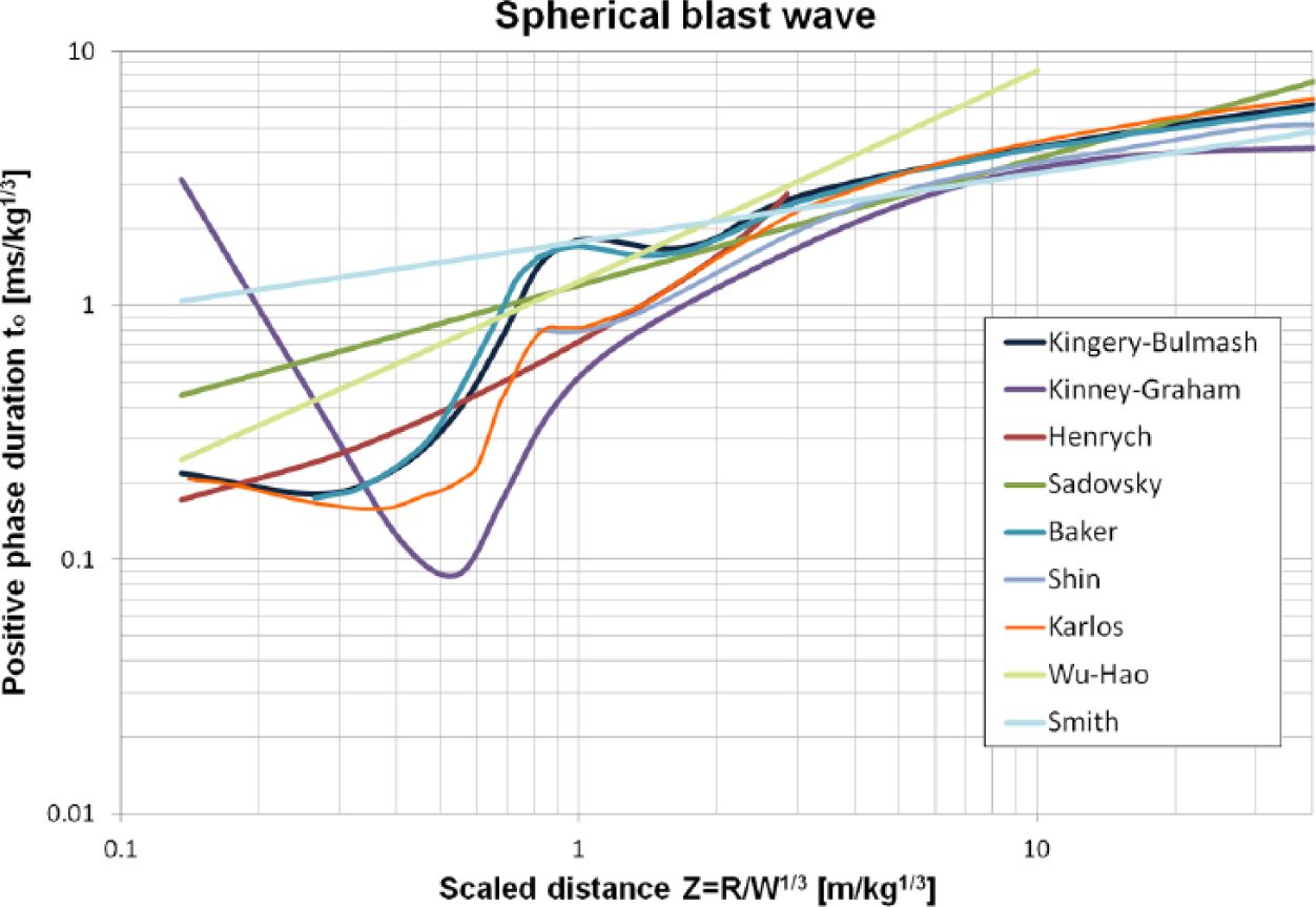
Comparison of positive phase duration values versus scaled distance for a spherical blast wave.

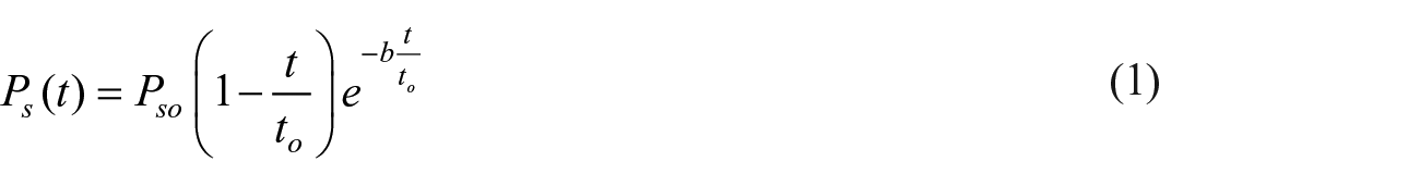
The determination of the blast parameters has been under investigation by various researchers over the last decades. As a result, there exist several equations and charts that are (mainly) based on the analysis of various experimental data. Most of the available equations have been produced for spherical bursts and incident blast waves as they constitute the most extensively studied case, for which the explosion is supposed to have taken place in mid-air and the created blast wave propagates spherically outward. Such formulations for calculating the incident wave parameters have been published by Brode (1955, 1956), Naumyenko and Petrovshyi (1956), Sadovsky (2004), Henrych (1979), Baker et al. (1983), Goodman (1960), Kinney and Graham (1985), Wu and Hao (2005), Mills (1987), Shin et al. (2015), Karlos and Solomos (2016), and others. As literature shows, the most widely accepted approach for determining the blast wave parameters is that of the technical manual by Kingery and Bulmash (1984). This source contains polynomial equations for calculating the main blast parameters of both incident and reflected blast waves from spherical and hemispherical bursts. Their metric version can be reproduced in the Unified Facilities Criteria (2008) and is included in Karlos and Solomos (2013). The relevant curves of the above formulations have been compiled and coherently compared below.

Figure 1 shows the peak positive incident overpressure values for a spherical blast in relation to the scaled distance according to the various sources. It can be observed that all proposed peak overpressure values are close for scaled distances in the range of 2 < Z < 20 m/kg^1/3, but for smaller scaled distances, a substantial difference appears among some of the curves. As noticed, the number of available relationships that describe the peak reflected overpressure is smaller than that of the incident case (Figure 1), even though the reflected overpressure is more important for design purposes. Equations for its calculation are provided by Kingery and Bulmash (1984), Shin et al. (2015), Smith and Hetherington (1994), Brode (1968), and Baker (1973).

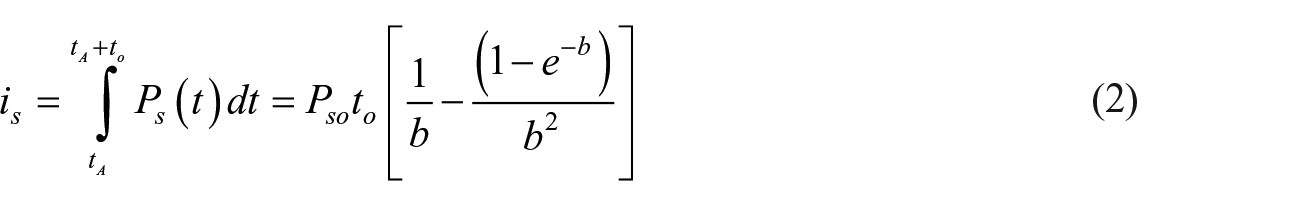
Figure 2 shows the variation of the scaled positive incident impulse for a spherical blast wave in relation to the scaled distance. The curve from Henrych singles out as it overpredicts the blast impulse by more than 200% with respect to the proposals of other researchers and is also characterized by a smaller scaled distance validity range. The rest of the examined relationships give similar results for larger scaled distances (Z > 1 m/kg^1/3), but some variations appear among them for smaller scaled distances. If the reflected impulse is of interest, there are again a limited number of available equations, and proposals for its calculation can be found in Kingery and Bulmash (1984), Shin et al. (2015), and Baker et al. (1983).

Figure 3 shows the scaled incident positive phase duration for a spherical blast wave in relation to the scaled distance. From the diagram, it appears that the blast duration is the parameter with the largest differences among curves, when compared to those of the peak overpressure and impulse. One of the reasons lies in the difficulty of calculating the positive duration from the available experimental data, as it proves hard to accurately define from a recorded pressure signal the point at which the blast pressure becomes equal to the ambient value.

Blast pressure decay coefficient formulations

According to the modeling of equation (1), the blast wave decay coefficient b is a dimensionless parameter and is essential for drawing the pressure–time history curve, as it describes the decrease rate of the pressure values. Different coefficient values should be used for designing the pressure–time history depending on whether the curve is for the incident or the reflected blast wave. The pressure decrease rate is not always the same in these two cases, as was shown by Chock and Kapania (2001).

There are several relationships available in the literature for calculating this coefficient by utilizing the rest of the blast parameters, mainly referred to the incident blast wave case. A series of such equations (or tables) can be found in Brode (1955), Kinney and Graham (1985), Baker et al. (1983), Larcher (2007), Lam et al. (2004), Borgers and Vantomme (2008), Teich and Gebbeken (2010), Dharaneepathy et al. (2006), Ismail and Murray (1993), and others. Figure 4 shows the variation of the decay coefficient of the incident wave in relation to the scaled distance for a free-air burst according to the described models. In cases where no relationship was suggested (Kingery and Bulmash, 1984; Sadovsky, 2004; Shin et al., 2015) the relevant decay coefficient curve was calculated by iteratively solving equation (2), while the peak overpressure, impulse, and duration were computed according to the formulations proposed from the relevant researchers. The domain of each decay coefficient curve coincides with the scaled distance limits set by each researcher.

Figure 4.

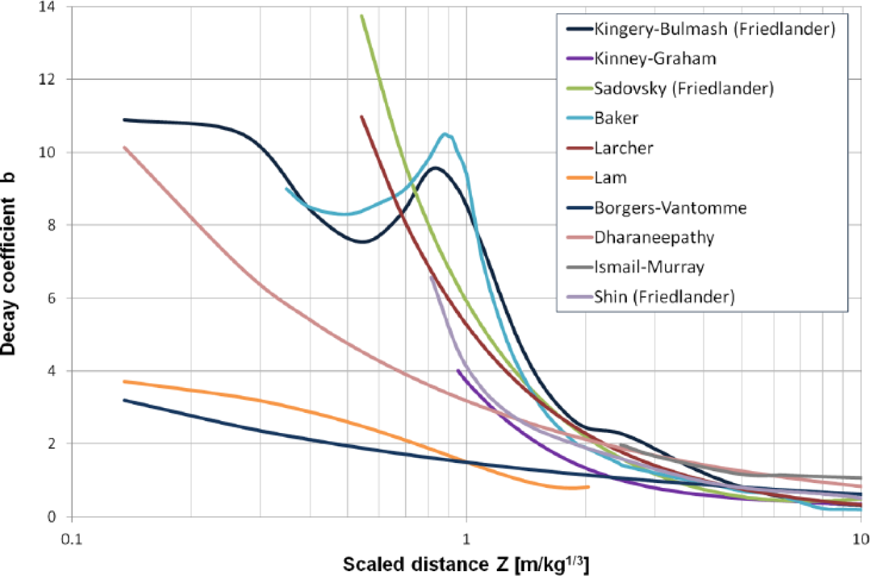
Variation of the decay coefficient with scaled distance for a free-air incident blast wave.

Figure 4 shows that for smaller scaled distances, the discrepancies among the different equations of the decay coefficient are significant. This should be also attributed to the scatter of the values of impulse, pressure, and blast duration among the various proposed relationships. Teich (2012) and Goel et al. (2012) provide diagrams that show the big differences among the blast parameters proposed by various researchers, pointing out the difficulty of precise measurements in extremely short phenomena like the explosions. The construction of the blast pressure–time history is a prerequisite for simulation purposes, as it determines the pressure that will be applied to an element at every time increment in an explicit finite element analysis. The decay coefficient is essential for drawing this curve and should be chosen in accordance with the set of equations that were used for calculating the rest of the blast parameters.

Decay coefficient using the Kingery–Bulmash parameters

As already pointed out, the technical report of Kingery and Bulmash (1984) has been extensively used by designers for calculating the loads generated after an explosion and its proposals have also been adopted in various military publications, such as the Unified Facilities Criteria (2008). The report contains polynomial equations and curves for both incident and reflected blast parameters from free-air and surface bursts. The available equations allow the calculation of the positive overpressure, the positive impulse, the shock front velocity, the arrival time, and the positive phase duration. There are no equations that describe the negative phase of the blast wave or for the calculation of the pressure decay coefficient. The analysis that follows aims at producing functional relationships for the decay coefficient for four idealized explosion categories: (a) incident spherical wave, (b) reflected spherical wave, (c) incident hemispherical wave, and (d) reflected hemispherical wave. Two relationships are proposed for every category: the first one being valid for smaller and the second for larger scaled distances.

Free-air bursts

Incident blast wave

For calculating the incident decay coefficient from a free-air burst, the Friedlander equation in the form of equation (2) is used. The blast parameters for a reference point are calculated through the polynomial equations of Kingery–Bulmash by examining a large combination of charge values and stand-off distances. The resulting values of peak overpressure, impulse, and positive phase duration (P_so, i_s, and t_o) are inserted into equation (2), which is solved iteratively, and a single b value is calculated for every blast configuration. These b points, joined by smooth curves, are plotted in Figure 5 in relation to the stand-off distance and the used charge. Such diagrams have been derived in this study for all four idealized explosion categories.

Figure 5.

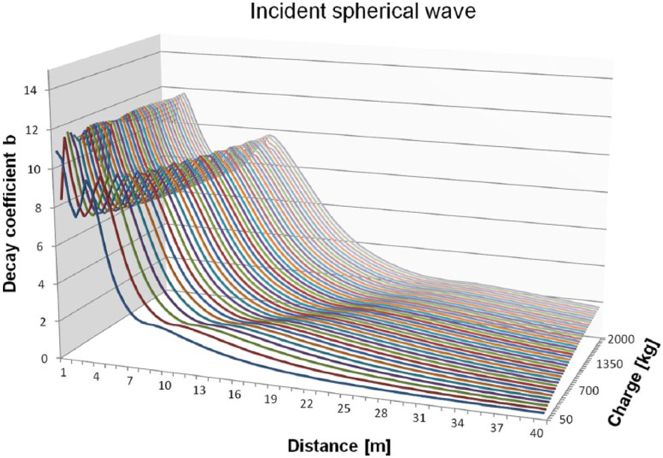
Incident spherical blast wave decay coefficient using the Kingery–Bulmash data and the Friedlander equation.

It is clearly evidenced in the analysis of the current and the next three cases that the graphs of the coefficient b, plotted as in Figure 5, coalesce into a graph of a single variable, the scaled distance Z. This could have been expected, as the parameter b is just a dimensionless constant in the Friedlander equation. Therefore, according to the scaling law used for modeling the explosion phenomenon, the b value should be the same for equal scaled distances. This property can also be proved through the following simple reasoning.

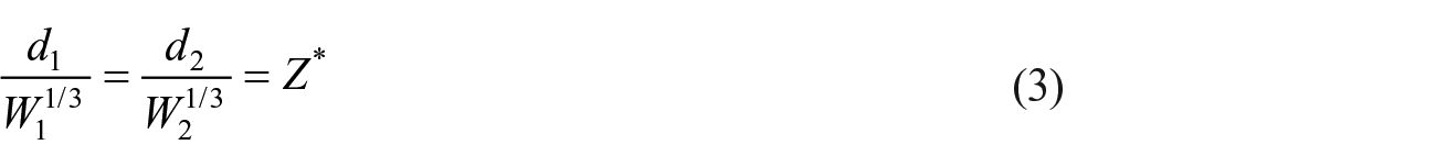
Two different explosive charges W₁ and W₂ are considered at stand-off distances d₁ and d₂, respectively, from a point of interest, such that their scaled distances are equal, that is

\frac{d_{1}}{W_{1}^{1 / 3}} = \frac{d_{2}}{W_{2}^{1 / 3}} = Z^{*}

(3)

For this Z*, through the appropriate Kingery–Bulmash curves (or equations), three parameters for the peak overpressure, positive impulse, and positive phase duration at this point are calculated: P_so, i_s*, and t_o* (* denotes scaled values).

Based on these, the corresponding actual values of the blast wave at the point due to the charges W₁ and W₂, respectively, would be

\begin{array}{l} P_{s o 1} = P_{s o}, i_{s 1} = i_{s}^{*} W_{1}^{1 / 3}, t_{o 1} = t_{o}^{*} W_{1}^{1 / 3} \\ P_{s o 2} = P_{s o}, i_{s 2} = i_{s}^{*} W_{2}^{1 / 3}, t_{o 2} = t_{o}^{*} W_{2}^{1 / 3} \end{array}

(4)

Using these values, the form of the pressure wave at the point of interest for each of the two charges would next be written in terms of a Friedlander equation (1). The corresponding decay parameters b₁ and b₂ would be determined using equation (2), specifically

\begin{array}{l} \frac{1}{b_{1}} - \frac{1}{b_{1}^{2}} (1 - e^{- b_{1}}) = \frac{i_{s 1}}{P_{s o 1} t_{o 1}} = \frac{i_{s}^{*} W_{1}^{1 / 3}}{P_{s o} t_{o}^{*} W_{1}^{1 / 3}} = \frac{i_{s}^{*}}{P_{s o} t_{o}^{*}} \\ \frac{1}{b_{2}} - \frac{1}{b_{2}^{2}} (1 - e^{- b_{2}}) = \frac{i_{s 2}}{P_{s o 2} t_{o 2}} = \frac{i_{s}^{*} W_{2}^{1 / 3}}{P_{s o} t_{o}^{*} W_{2}^{1 / 3}} = \frac{i_{s}^{*}}{P_{s o} t_{o}^{*}} \end{array}

(5)

As is immediately evident, the constants b₁ and b₂ are determined through two equations which are identical, and therefore, it can be concluded, as initially claimed that

b_{1} = b_{2}

(6)

The fitting of the calculated (b, Z) points by an analytical expression is attempted next. It is, however, reminded that the Kingery and Bulmash (1984) technical manual provides recommendations for the spherical blast parameters for Z > 0.053 m/kg^1/3 and for the hemispherical ones for Z > 0.067 m/kg^1/3 (for the positive phase duration, it is Z > 0.147 m/kg^1/3 and Z > 0.178 m/kg^1/3, respectively). But as shown by Shin et al. (2015), the supporting experimental data at such small scaled distance values are limited and of ambiguous quality. Bogosian et al. (2002) also showed that at smaller scaled distances, there exist considerable differences between the Kingery–Bulmash curve and several experimental results for incident and reflected blast waves. This means that treating the Kingery–Bulmash proposals at the near-field as reference values would introduce big uncertainties and should be avoided. Also, various studies (Shin et al., 2015; Smith and Hetherington, 1994) have shown that the Friedlander equation cannot be successfully used at smaller scaled distances, as the form of the pressure–time curve is different than the idealized shape suggested by equation (1). This is attributed to the effect of the expanding detonation products that result in overpressure diagrams with multiple peaks (associated with the arrival of the blast front and the detonation products). Thus, this study focuses on a scaled distance range 0.4 ⩽ Z < 40.0 m/kg^1/3 where the blast parameter values from the various sources are acceptably accurate, and the effect of the expanding detonation products is less evident. Nevertheless, the proposed decay coefficients for Z < 1.0 m/kg^1/3 should be used with caution because of the uncertainties involved when trying to calculate the blast parameters at such short distances from the detonation center. It is noted that the development of new experimental techniques for measurements of close-in explosions (Rigby et al., 2015b) could increase the level of confidence of the blast parameter values at such distances.

For fitting the calculated decay coefficient-scaled distance points, the curve is divided in two parts, as its complex shape makes difficult the use of a single equation. The first part of the curve is valid for smaller scaled distances, 0.4 ⩽ Z < 2.0 m/kg^1/3, and the second part for larger ones, 2.0 ⩽ Z < 40.0 m/kg^1/3. The fitting equations are expressed through polynomial relationships similar to those employed by Kingery and Bulmash (1984) when describing the rest of the blast parameters. Their form is described by equation (7)

Y = C_{0} + C_{1} U + C_{2} U^{2} + \dots + C_{n} U^{n} with U = K_{0} + K_{1} T

(7)

where Y is the common logarithm of the decay coefficient, T is the common logarithm of the scaled distance, and N is the polynomial’s order. The constants {K₀, K₁, C₀, C₁ … C_n} are defined through the least-squares fitting of the calculated b-coefficient values, and the polynomial’s order is selected so that the difference from the analysis values is smaller than 3%.

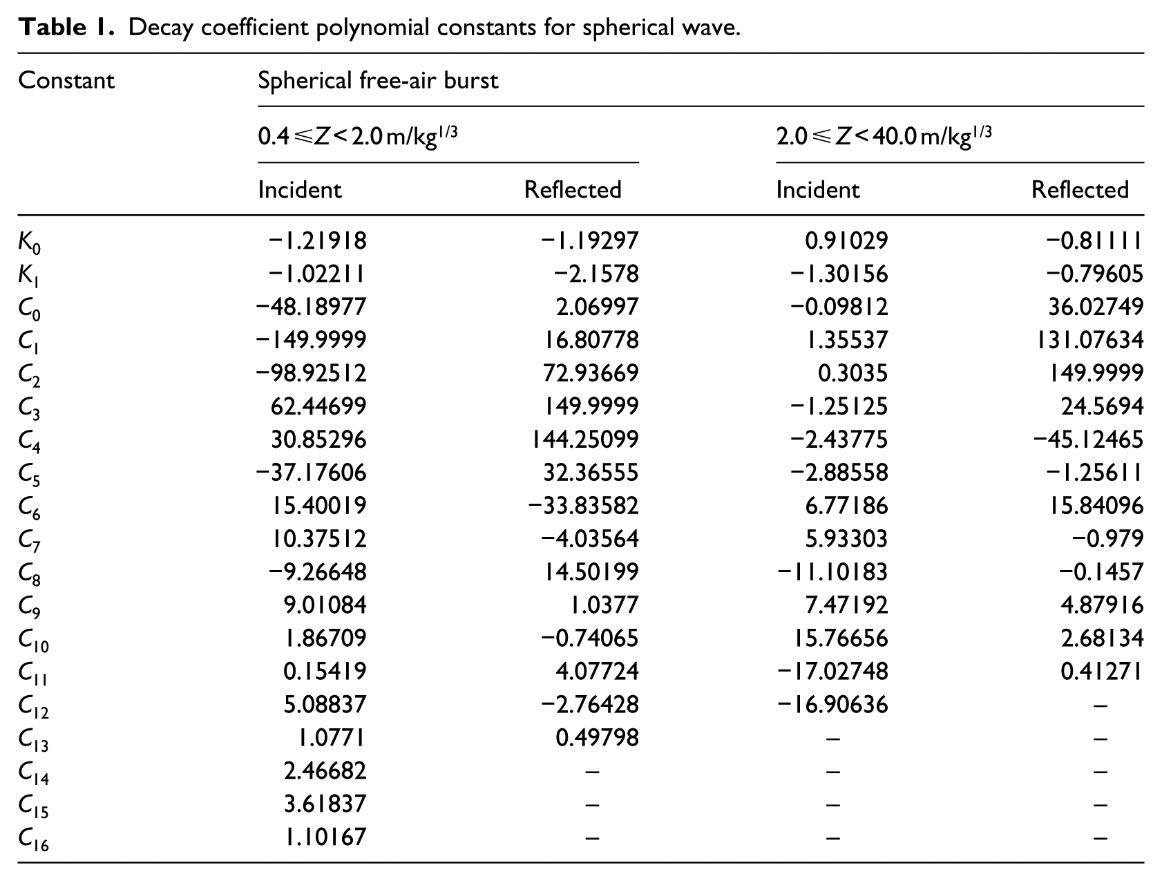
For the case of the spherical incident blast wave, the derived values of the constants {K₀, K₁, C₀, C₁ … C_n} are included in Table 1. Figure 6 shows also in detail the nonlinear fit with the above analytical expressions of the calculated points of the decay coefficient, where the goodness of fit appears to be very good. It is in particular noted that the value of b at the domain division point Z = 2.0 m/kg^1/3, calculated by the respective equations (7), is b(2.0⁻) = 2.49 and b(2.0⁺) = 2.42, that is, identical for all practical purposes.

Table 1.

Decay coefficient polynomial constants for spherical wave.

Constant	Spherical free-air burst
	0.4 ⩽Z < 2.0 m/kg^1/3		2.0 ⩽ Z < 40.0 m/kg^1/3
	Incident	Reflected	Incident	Reflected
K ₀	−1.21918	−1.19297	0.91029	−0.81111
K ₁	−1.02211	−2.1578	−1.30156	−0.79605
C ₀	−48.18977	2.06997	−0.09812	36.02749
C ₁	−149.9999	16.80778	1.35537	131.07634
C ₂	−98.92512	72.93669	0.3035	149.9999
C ₃	62.44699	149.9999	−1.25125	24.5694
C ₄	30.85296	144.25099	−2.43775	−45.12465
C ₅	−37.17606	32.36555	−2.88558	−1.25611
C ₆	15.40019	−33.83582	6.77186	15.84096
C ₇	10.37512	−4.03564	5.93303	−0.979
C ₈	−9.26648	14.50199	−11.10183	−0.1457
C ₉	9.01084	1.0377	7.47192	4.87916
C ₁₀	1.86709	−0.74065	15.76656	2.68134
C ₁₁	0.15419	4.07724	−17.02748	0.41271
C ₁₂	5.08837	−2.76428	−16.90636	−
C ₁₃	1.0771	0.49798	−	−
C ₁₄	2.46682	−	−	−
C ₁₅	3.61837	−	−	−
C ₁₆	1.10167	−	−	−

Figure 6.

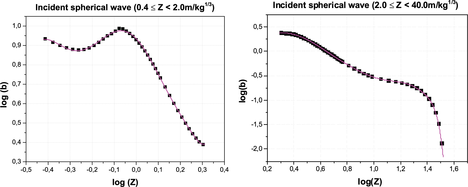
Incident spherical blast wave decay coefficients in relation to the scaled distance for 0.4 ⩽ Z < 2.0 m/kg^1/3 (left) and 2.0 ⩽ Z < 40.0 m/kg^1/3 (right).

Reflected blast wave

Equation (2) is again used for the calculation of the decay coefficient for the reflected blast wave. As a rule, the incident and the reflected blast waves have different decay coefficients even if they refer to the same scaled distance. It is only interesting to observe that if the ratio of the peak reflected and incident overpressures was equal to the ratio of the reflected and incident positive impulses, equation (2) would yield identical decay coefficient values for the two cases, since the positive phase duration is common. This is rarely the case in the Kingery–Bulmash data.

As in the above case of the incident wave, a large number of charge and stand-off distance combinations are studied, and the corresponding blast parameters P_ro, i_r, and t_o are calculated through the relevant Kingery–Bulmash polynomial equations. Accordingly, these parameters are substituted into equation (2) which is solved iteratively and a single decay coefficient is estimated for each case. As before, a graph similar to that of Figure 5 is produced, which is next reduced to a series of (Z, b) points, and then fitted by equation (7). The fitting curve is again divided in two parts, and the constants involved are determined and shown in Table 1. The value of b at the domain division point Z = 2.0 m/kg^1/3 calculated by the respective equations (7) is b(2.0⁻) = 3.70 and b(2.0⁺) = 3.69, that is, practically identical.

Surface bursts

The pressure–time curve of a surface burst is different from the same-charge curve of a free-air burst because of the instantaneous interaction of the blast wave with the ground. Occasionally, blast manuals consider this phenomenon by applying an amplification factor of 1.7–1.8 to the actual charge weight and using the resulting free-air burst parameter values. The produced hemispherical wave has practical importance for designers, since large explosive charges from terrorist attacks are expected to be placed at approximately ground level.

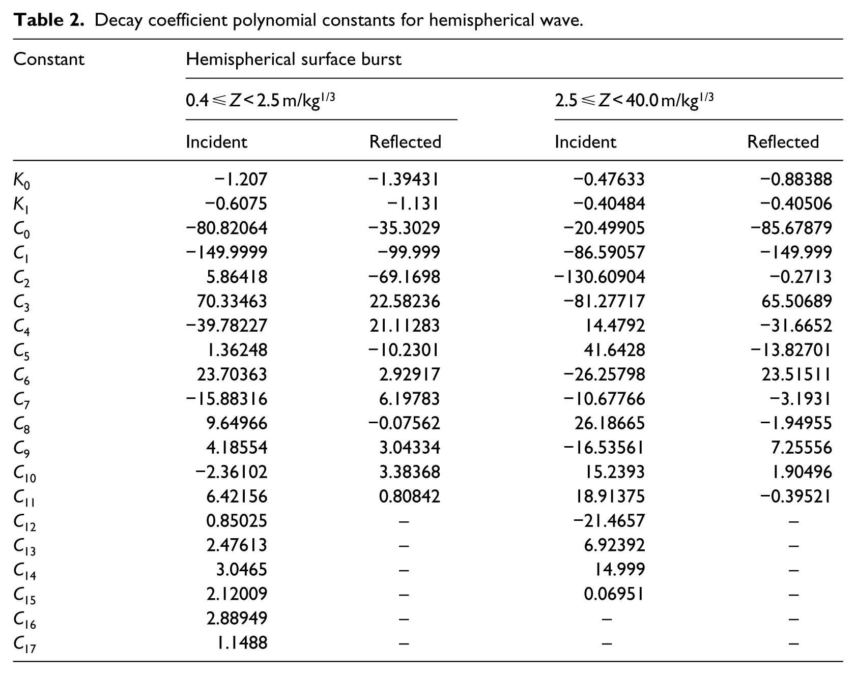
Following the previous procedure, the decay coefficients for both the incident and the reflected blast waves are calculated by iteratively solving equation (2) for various sets of blast parameters. The produced set of decay coefficient-scaled distance points, is fitted in each case by equation (7), and the scaled-distance domain is again divided in two parts, one for smaller, 0.4 ⩽ Z < 2.5 m/kg^1/3, and the other for larger values, 2.5 ⩽ Z < 40.0 m/kg^1/3. The values of the constants {K₀, K₁, C₀, C₁ … C_n}, derived through these least-squares fittings, are reported in Table 2. The goodness of fit and the continuity at the domain division point Z = 2.5 m/kg^1/3 are again checked and found excellent.

Table 2.

Decay coefficient polynomial constants for hemispherical wave.

Constant	Hemispherical surface burst
	0.4 ⩽ Z < 2.5 m/kg^1/3		2.5 ⩽ Z < 40.0 m/kg^1/3
	Incident	Reflected	Incident	Reflected
K ₀	−1.207	−1.39431	−0.47633	−0.88388
K ₁	−0.6075	−1.131	−0.40484	−0.40506
C ₀	−80.82064	−35.3029	−20.49905	−85.67879
C ₁	−149.9999	−99.999	−86.59057	−149.999
C ₂	5.86418	−69.1698	−130.60904	−0.2713
C ₃	70.33463	22.58236	−81.27717	65.50689
C ₄	−39.78227	21.11283	14.4792	−31.6652
C ₅	1.36248	−10.2301	41.6428	−13.82701
C ₆	23.70363	2.92917	−26.25798	23.51511
C ₇	−15.88316	6.19783	−10.67766	−3.1931
C ₈	9.64966	−0.07562	26.18665	−1.94955
C ₉	4.18554	3.04334	−16.53561	7.25556
C ₁₀	−2.36102	3.38368	15.2393	1.90496
C ₁₁	6.42156	0.80842	18.91375	−0.39521
C ₁₂	0.85025	−	−21.4657	−
C ₁₃	2.47613	−	6.92392	−
C ₁₄	3.0465	−	14.999	−
C ₁₅	2.12009	−	0.06951	−
C ₁₆	2.88949	−	−	−
C ₁₇	1.1488	−	−	−

Decay coefficient comparison

Figure 7 shows the pressure decay coefficients for all of the above cases in relation to the scaled distance in a logarithmic scale diagram. A similarity can be noted in the shapes between the two incident and the two reflected wave curves, respectively. The difference between the incident and reflected decay coefficient values is attributed to the fact that the resulting values are based on a numerical elaboration, through equation (2), of empirical data on P_so, i_s, and t_o (or P_ro, i_r, and t_o) according to Kingery and Bulmash (1984). It is the relative magnitudes of these three parameters (whose behavior is quite peculiar, as shown in Figures 1 to 3) that govern the value derived for the coefficient b. It should also be noted that the Friedlander equation is not a purely exponential function, but it contains a multiplicative linear term of time. For facilitating their use, the values of these curves are reported in tabular form in the Appendix 1.

Figure 7.

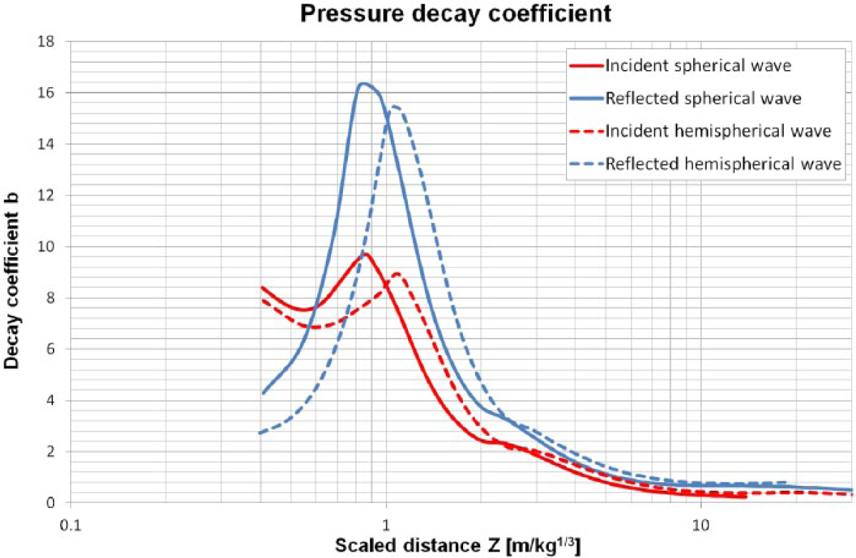
Incident and reflected blast wave decay coefficients for a free-air and a surface burst.

Assessment of derived expressions

Comparison with experimental data

The determination of the decay coefficient has been based entirely on the relationships included in the technical report of Kingery and Bulmash (1984). Even though the equations proposed in Kingery and Bulmash (1984) are based on data from many different sources, such as Kingery (1966) and Kingery and Coulter (1983), as pointed out from Ngo et al. (2015), they include uncertainties which are mainly attributed to the lack of proper measuring instruments when the experiments took place. Consequently, it could prove useful to make a comparison with decay coefficient values whose calculation is based on recent experiments with more accurate measurements. Two sets of such data are utilized below.

A series of experiments was performed at the Blast & Impact Laboratory in Buxton at the University of Sheffield, Sheffield, UK, that is described in Rigby et al. (2015a). Explosive charges of PE4 (1.2 TNT equivalence factor) were placed on the ground at various distances from a rigid concrete wall, and after detonation, the resulting reflecting pressures from the hemispherical blast wave were measured at four different locations on the wall. The first point was located directly across the detonation point and was subjected to the fully reflected normal overpressure, while the rest of the measuring locations were at an angle to the blast wave propagation direction. As was reported in Rigby et al. (2015a), the experimentally defined blast parameters for the normally reflected case had a very good agreement with the parameters proposed in Unified Facilities Criteria (2008).

The second set consists of experimental incident blast wave parameters that are included in Ngo et al. (2015) and have been acquired from a large-scale explosion that took place in Woomera in South Australia. The charge was cylindrically shaped and consisted of 5000 kg of TNT placed on the ground resulting in the creation of a hemispherical blast wave. The incident pressure was measured from pressure transducers that were positioned parallel to the direction of the propagating wave. The recordings were performed along two lines placed at a 90° angle, from pairs of transducers positioned at identical distances from the detonation point. As pointed out in Ngo et al. (2015), the readings from the pairs of transducers show a big variation, which suggests that the propagation of the blast wave was not symmetrical.

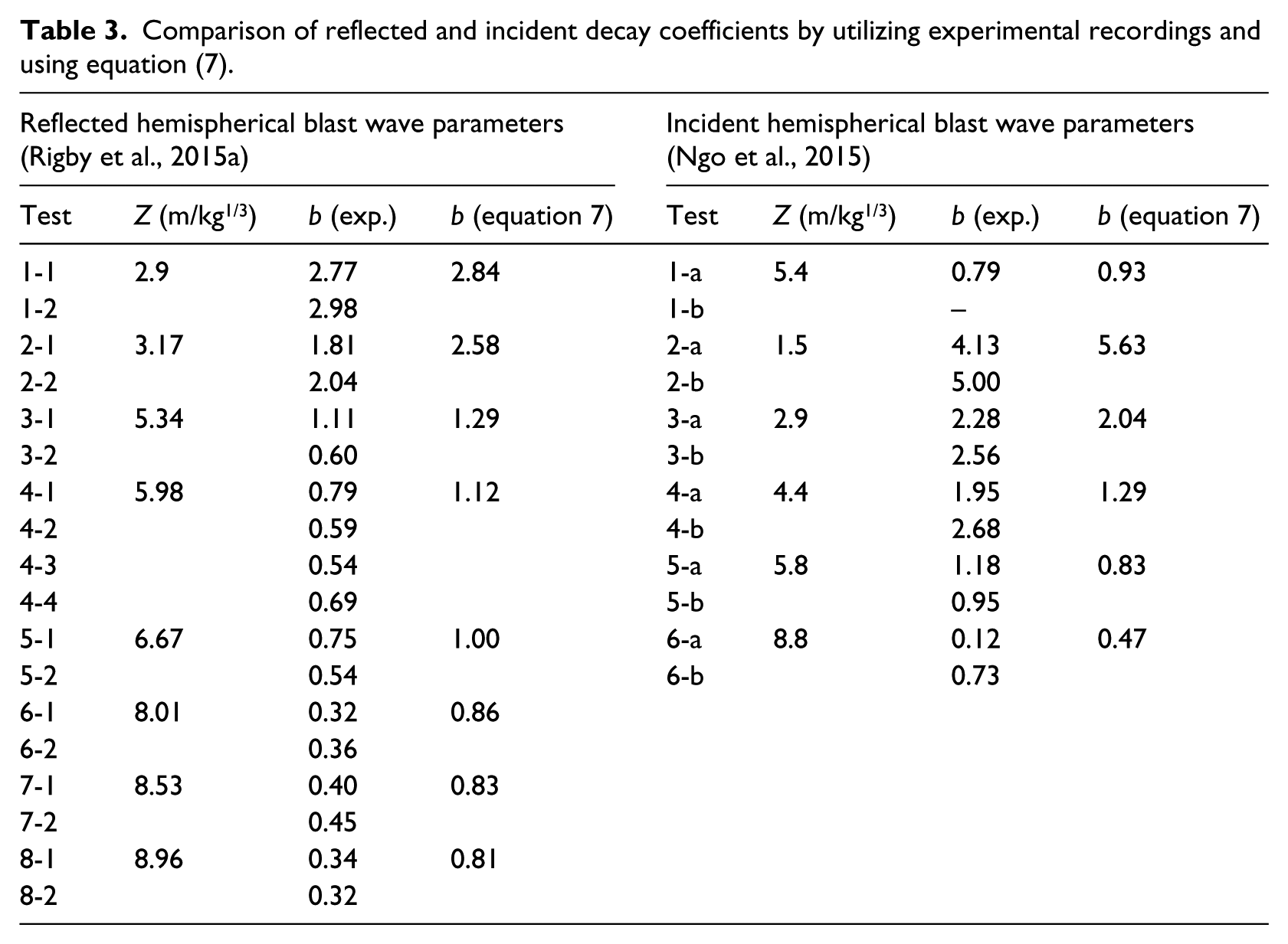
Table 3 shows the calculated decay coefficients for the above-mentioned experiments. For each case, two coefficients were computed, the first one by utilizing the experimental recordings and equation (2), and the second using equation (7).

Table 3.

Comparison of reflected and incident decay coefficients by utilizing experimental recordings and using equation (7).

Reflected hemispherical blast wave parameters (Rigby et al., 2015a)				Incident hemispherical blast wave parameters (Ngo et al., 2015)
Test	Z (m/kg^1/3)	b (exp.)	b (equation 7)	Test	Z (m/kg^1/3)	b (exp.)	b (equation 7)
1-1	2.9	2.77	2.84	1-a	5.4	0.79	0.93
1-2		2.98		1-b		−	0.93
2-1	3.17	1.81	2.58	2-a	1.5	4.13	5.63
2-2		2.04		2-b		5.00	5.63
3-1	5.34	1.11	1.29	3-a	2.9	2.28	2.04
3-2		0.60		3-b		2.56	2.04
4-1	5.98	0.79	1.12	4-a	4.4	1.95	1.29
4-2		0.59		4-b		2.68	1.29
4-3		0.54		5-a	5.8	1.18	0.83
4-4		0.69		5-b		0.95	0.83
5-1	6.67	0.75	1.00	6-a	8.8	0.12	0.47
5-2		0.54		6-b		0.73	0.47
6-1	8.01	0.32	0.86
6-2		0.36
7-1	8.53	0.40	0.83
7-2		0.45
8-1	8.96	0.34	0.81
8-2		0.32

The diagram in Figure 8 shows the comparison between the decay coefficient values included in Table 3. At this scatter plot, the x-axis represents the values calculated through equation (7), and the y-axis represents those obtained from utilizing the experimental readings. Even though the expected trend is followed, the plot shows that the derived decay values may have substantial differences. This is especially the case for the incident blast wave, where the bigger discrepancies may be attributed, according to Ngo et al. (2015), to the asymmetrical nature of the blast wave propagation.

Figure 8.

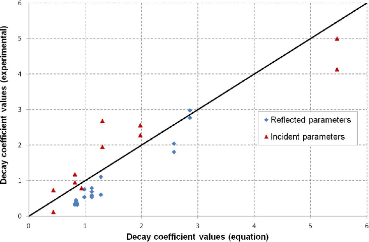
Scatter plot of the decay coefficient values for reflected and incident blast wave parameters.

Sensitivity analysis and trends

The substantial variability of the blast parameters has been noted by various researchers even for identical field experiments. In their work, Netherton and Stewart (2010), Bogosian et al. (2002), Campidelli et al. (2015), and Twisdale et al. (1993) showed that in some cases, the peak overpressure and positive impulse can differ by more than 40% (and the positive duration by more than 60%) in relation to the proposed values by Kingery and Bulmash (1984). Their analyses utilized results from field tests, some of which were conducted several decades ago. The uncertainties in the parameters were related to the variability in stand-off distance, charge mass, atmospheric conditions, ground morphology, and so on. But, if the experiments (far-field) are performed in a well-controlled environment, it has been shown by Rigby et al. (2014b) that the results can have a high degree of consistency and repeatability, which means that the inherent variation of blast parameters is very low and could be attributed to other factors (instrumentation, environmental conditions, etc.).

This degree of uncertainty when deriving a blast parameter using a technical manual naturally affects to some extent the calculated decay coefficient values. The influence of the uncertainties in each blast parameter on the decay coefficient value can be quantified through a sensitivity analysis. During this analysis, for a specific loading case, a deterministic analysis is first conducted with the Kingery–Bulmash provided values for the positive phase peak overpressure, impulse, and duration, and the value of the decay coefficient is calculated through equation (2). Subsequently, one of the three parameters (i.e. P_ro, i_r, and t_o) in the Friedlander equation is assumed to be a random variable, and the decay coefficient is recalculated, while the other two parameters remain deterministic and equal to their previously calculated value. The case of all three parameters varying simultaneously is also examined.

The decay coefficient for each blast parameter set is calculated through a Monte Carlo scheme, and the sensitivity of each parameter is finally defined by comparing the difference between the deterministic and probabilistic value of the decay coefficient.

The available information about the randomness of each blast parameter is limited. In Borenstein and Benaroya (2009), they have been assumed to be uniformly distributed, while other researchers (Twisdale et al., 1993), based on a number of experimental recordings made from surface detonations of general-purpose bombs, have showed that the probability of these parameters follows a log-normal distribution. At this study, the random variable parameters are considered to follow uniform distributions (the procedure would not change if a normal or log-normal distribution were considered). The adoption of a uniform distribution implies that we have some knowledge regarding the upper and lower bounds of the parameter values, but we do not know how their values are distributed inside these bounds.

The mean value of the uniform distribution for each blast parameter is provided by the Kingery and Bulmash (1984) relationships, its range denoted by RA is defined as the range between the parameter’s upper and lower values, and its standard deviation σ is calculated by equation (8)

σ = \frac{R A}{\sqrt{12}}

(8)

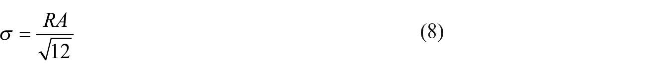
Each blast parameter (i.e. peak overpressure, impulse, and duration) takes random values X generated through equation (9)

Χ = Χ_{m} + (R A / 2) (2 \cdot r a n d - 1)

(9)

where X_m is the mean value of the parameter, RA is its range (symmetric about X_m), and rand is a random uniformly distributed number between 0 and 1, which is generated through the use of the software MATLAB. More than 10⁶ random samples are generated in each run. The parameter range RA is a measure of the spread and of the uncertainty of the random variable X; the larger the range, the greater the uncertainty in the parameter value. The range can also be conveniently expressed as a fraction of the mean value X_m, indicating this way the scatter of the parameter around its mean. For instance, if RA is chosen to be RA = 0.4 X_m, then the random parameter values X generated by equation (9) would fall uniformly in the interval (X_m−0.2 X_m, X_m + 0.2 X_m) = (0.8 X_m, 1.2 X_m).

The analysis performed in this section utilizes the data and the experimental setup from the tests included in Table 3. Specifically, Test 1-1 is chosen as input for the first random variable analysis. The experimental configuration consists of a 0.3 kg (TNT equivalent) charge positioned on the ground at a 2 m distance from a vertical stiff wall, on which proper instrumentation has been placed for the measurement of the reflected parameters of the blast wave. As outlined above, for each run, one blast parameter is chosen as the random variable and its mean value X_m is calculated according to Kingery and Bulmash (1984) and a range RA is defined. For each random value X from equation (9), a decay coefficient value is next calculated utilizing equation (2), and at the end, the average of all these calculated values is taken. This is the value designated as the mean decay coefficient for a specific range RA in the comparisons below. Runs have also been conducted where all three parameters are randomized simultaneously.

Figure 9 (left) shows the calculated decay coefficients when the range of the random peak overpressure and positive impulse is equal to 30% of their respective mean value (i.e. RA/2 = 0.15 X_m). The range of the random positive phase duration is 40% of its mean value (i.e. RA/2 = 0.20 X_m). These variability ranges of the blast parameters were chosen as representative of values reported in Netherton and Stewart (2010), Campidelli et al. (2015), and Twisdale et al. (1993). The procedure remains the same if the bands of the sensitivity analysis are tightened, following the suggestions of Rigby et al. (2014b), in which case the range of decay coefficient values would be significantly narrower.

Figure 9.

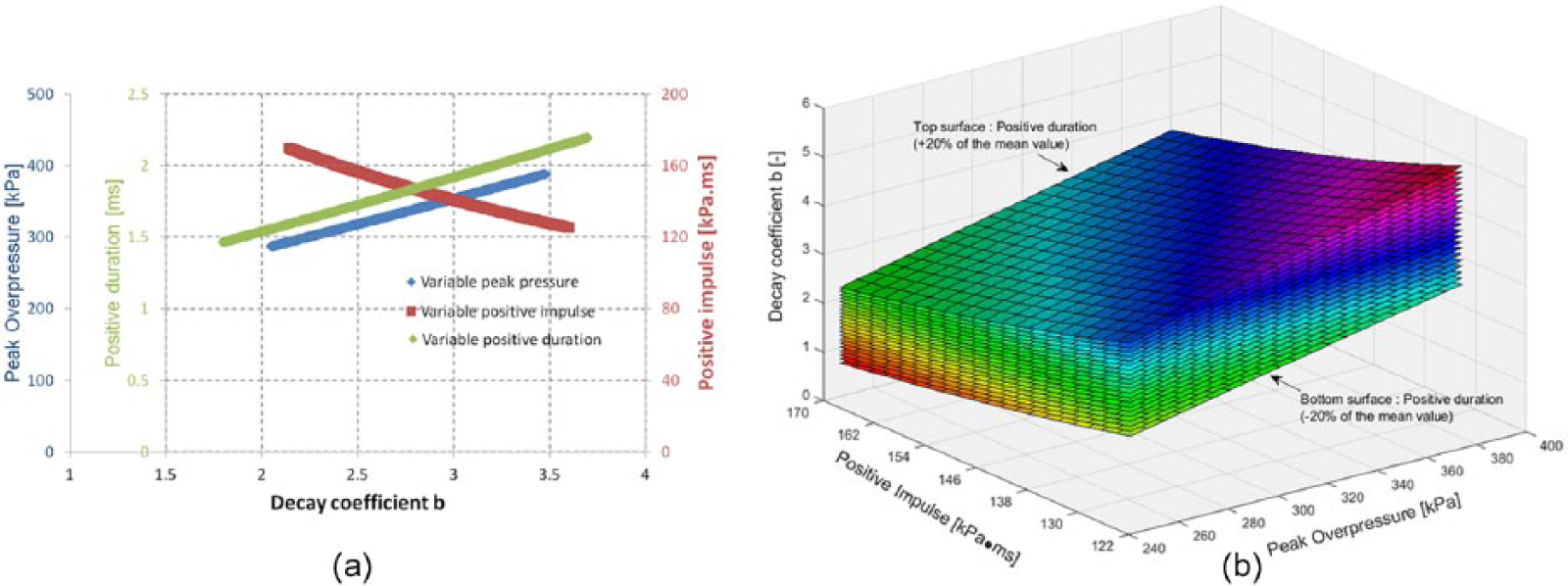
Mean decay coefficient values when only one of the blast parameters is randomized (left), and when all three parameters are considered random variables (right) for Test 1-1, for range of parameters of 30% of their mean value.

Figure 10 shows the calculated mean decay coefficient values, as the uncertainty of each blast parameter increases (i.e. increase in its range) for Test 1-1 for the specific case of RA = 0.4 X_m for all parameters. The mean decay coefficient values are plotted against a normalized variable which is equal to each variable parameter’s half range divided by its mean value. From this diagram, the influence of each blast parameter to the decay coefficient value can be readily assessed. It is seen that the mean decay coefficient tends to increase when the uncertainty of the impulse increases, and the rest of the parameters remain equal to their deterministic mean values. If, respectively, the uncertainty of the peak overpressure or of the positive duration increases (and the positive impulse is kept equal to its mean value), the mean decay coefficient remains almost invariable. If finally all three blast parameters are considered random, with the same respective range, the mean decay coefficient increases as the uncertainty (or the range) becomes larger.

Figure 10.

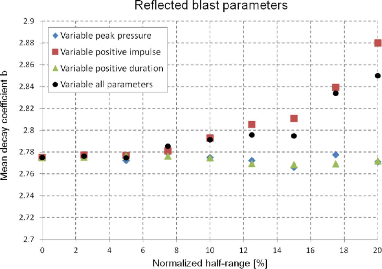
Mean decay coefficient behavior for random variable blast parameters for Test 1-1.

Figure 10 can be presented in the form of Table 4 that shows the percent error of the calculated mean decay coefficient values in relation to their corresponding deterministic values for various blast parameter ranges. The calculated error can be used as a measure of the sensitivity of each blast parameter to uncertainty. The results show that for some cases, an increase in the range of a parameter can lead to an increase at the percent error of the mean decay coefficient value. This tendency is recorded whenever either the positive impulse alone or all of the blast parameters are treated as random variables, as was observed in Figure 10. If only the peak positive overpressure or the blast positive duration are treated as random variables, the mean decay coefficient remains almost constant irrespective of the parameter range.

Table 4.

Percent errors of the calculated mean decay coefficient values.

Half range (%)	Blast parameters (Test 1-1, Z = 2.9 m/kg^1/3)
	P_r	i_r	t_o	All
2.5	0.09	0.08	0.02	0.05
5.0	0.10	0.07	0.06	0.01
7.5	0.15	0.22	0.05	0.37
10.0	0.01	0.64	0.01	0.59
12.5	0.10	1.10	0.20	0.75
15.0	0.32	1.29	0.23	0.70
17.5	0.10	2.32	0.21	2.13
20.0	0.14	3.78	0.11	2.70

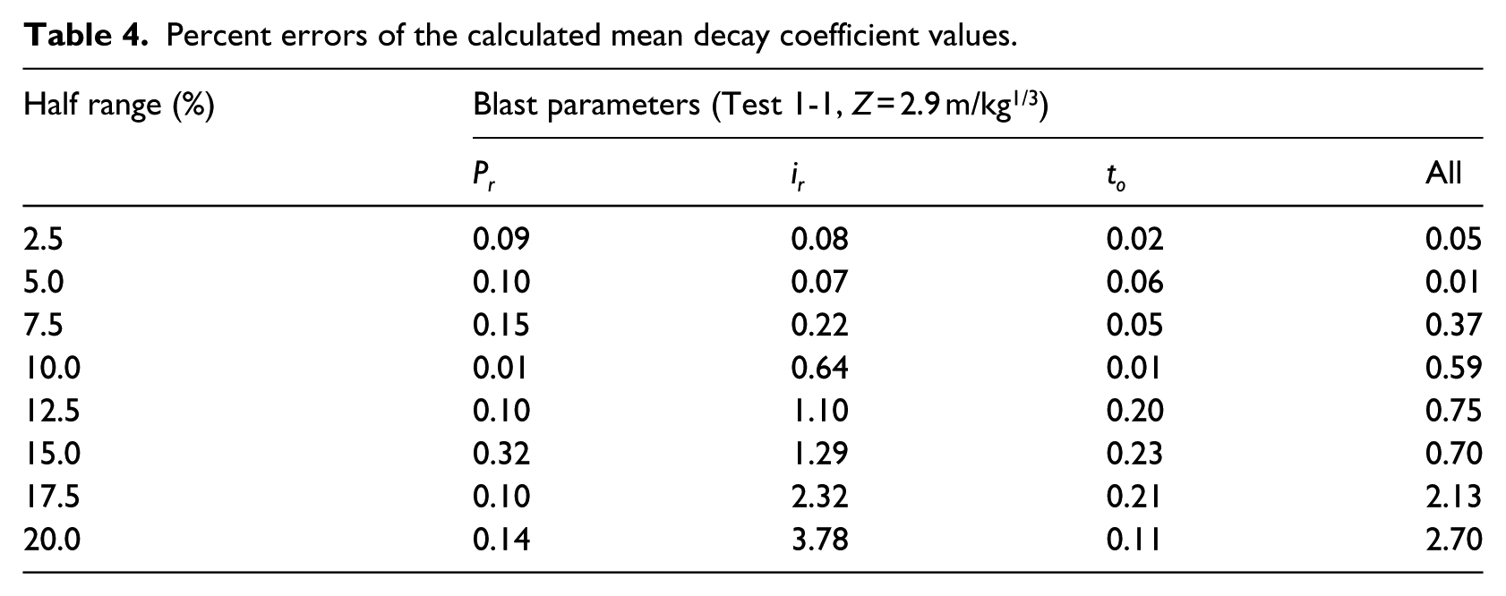
Figure 11 shows the probability density functions of the calculated mean decay coefficient for Test 1-1 when the relevant ranges are chosen as above. The histograms show that the probability density functions follow an almost uniform distribution when the blast peak overpressure or the positive duration parameters are treated as random parameters. When the blast positive impulse is the random parameter, the form of the probability density function indicates that there is greater probability for the decay coefficients to have smaller values. These Monte Carlo simulation results can be also analytically verified by starting with the uniform distribution of the parameter P_ro (or i_r, or t_o) and through transforming variables using equation (2) to determine the distribution of the parameter b. If all three blast parameters are considered simultaneously random, the decay coefficient probability density function follows a unimodal distribution but with more dispersed b values.

Figure 11.

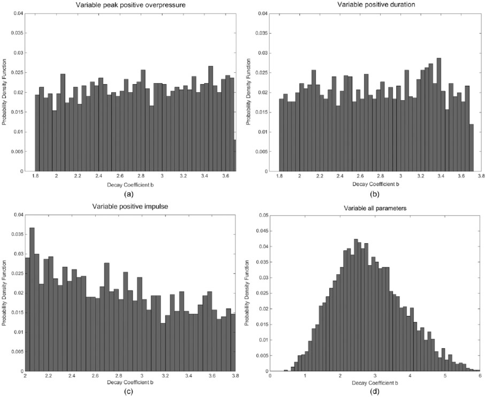
Probability density functions of decay coefficient for Test 1-1 when the variable blast parameter is (a) the peak overpressure, (b) the positive duration, (c) the positive impulse, and (d) all three of these parameters.

Figure 9 can help in understanding the shapes of these probability density functions. It is seen that when the peak overpressure or the positive duration are the varying parameters, the calculated decay coefficient increases in a linear mode. When the blast positive impulse is varied, the decay coefficient decreases following a concave-up curve. This means that the greater the scatter of the impulse, the greater the decay coefficient value will be in comparison to its deterministic value.

This can also be seen from the increase in the percent error in Table 4, when the uncertainty of the positive impulse increases. Furthermore, the slope of the impulse–decay coefficient curve decreases with increasing decay coefficient values, which indicates that if a certain impulse distribution range is considered, the scatter of the decay coefficient values will be smaller for larger impulse values (small b value region) and larger for smaller impulse values (large b value region). This explains the reason why the probability density function diagram in Figure 11 decreases while we move from the smaller to the larger decay coefficient region.

From the analyses performed, it is shown that overall the calculation of the blast decay coefficient is most sensitive to the uncertainties regarding the positive impulse, which thus must be measured or calculated with the best possible precision. The results of various tests, like those included in Table 3, have shown that the blast parameter with the greatest uncertainty is usually the wave positive duration (Borgers and Vantomme, 2008; Esparza, 1986). The positive impulse can generally be estimated with better accuracy, a fact that is beneficial for the calculation of the decay coefficient.

Conclusion

For determining the loading when designing a structure to sustain a blast, engineers have to rely on a set of available empirical or semi-empirical equations, tables, and graphs from various sources. This way, the needed blast parameters for the design such as peak overpressure, impulse, positive phase duration can be calculated. This study has reviewed some of the most commonly used relationships for the main blast parameters and has made a comparison of the corresponding resulting values. It has also been concluded that the Kingery–Bulmash set of equations can be treated as a reliable base for further analysis, due to its completeness and its supporting large experimental database.

Attention has next been focused on calculating the blast wave decay coefficient, which is necessary for plotting the pressure–time curve in the form of the Friedlander equation. As pointed out, the Kingery–Bulmash formulations do not provide an equation for this. Thus, a review of the available technical literature concerning the blast wave decay coefficient has been conducted and shown that the available expressions exhibit very large variations and are of limited use.

Finally, in the study, equations for the decay coefficient for both incident and reflected wave cases and for free-air and surface bursts have been developed using the Friedlander equation and inserted in the EUROPLEXUS (2013) explicit software. The proposed relationships are based on curve fitting of Kingery–Bulmash-derived data and are expressed as functions of the scaled distance. They are of polynomial form and their accuracy has been successfully assessed. Thus, an internally consistent set of equations has been created within the Kingery–Bulmash data framework. This certainly presents advantages regarding the consistency of the calculated pressure history at a point, which is to be inserted into a computer code for studying the effects of an explosion on a structure.

Additionally, a sensitivity analysis of the blast parameters included in the Friedlander equation has been conducted, and the results have shown that the positive impulse is the parameter whose uncertainty has the strongest influence on the calculated decay coefficients. The degree of uncertainty in the positive phase duration or in the peak positive overpressure has a smaller influence.

Of course, it is recalled that the whole formulation refers to the positive phase of the blast wave curve. Also the derived equations are restricted to scaled distances greater than Z = 0.4 m/kg^1/3. For close-in detonations, the Friedlander equation does not anymore represent the blast overpressure profile, and the decay parameter b is meaningless. In this region, where violent gas outflows and afterburning phenomena may take place, one would have to resort to computational fluid dynamics (CFD) techniques for determining the pressure–time history and definitely more experimental results would be necessary.

Footnotes

Appendix 1

Table 5.

Decay coefficient values for various scaled distance values.

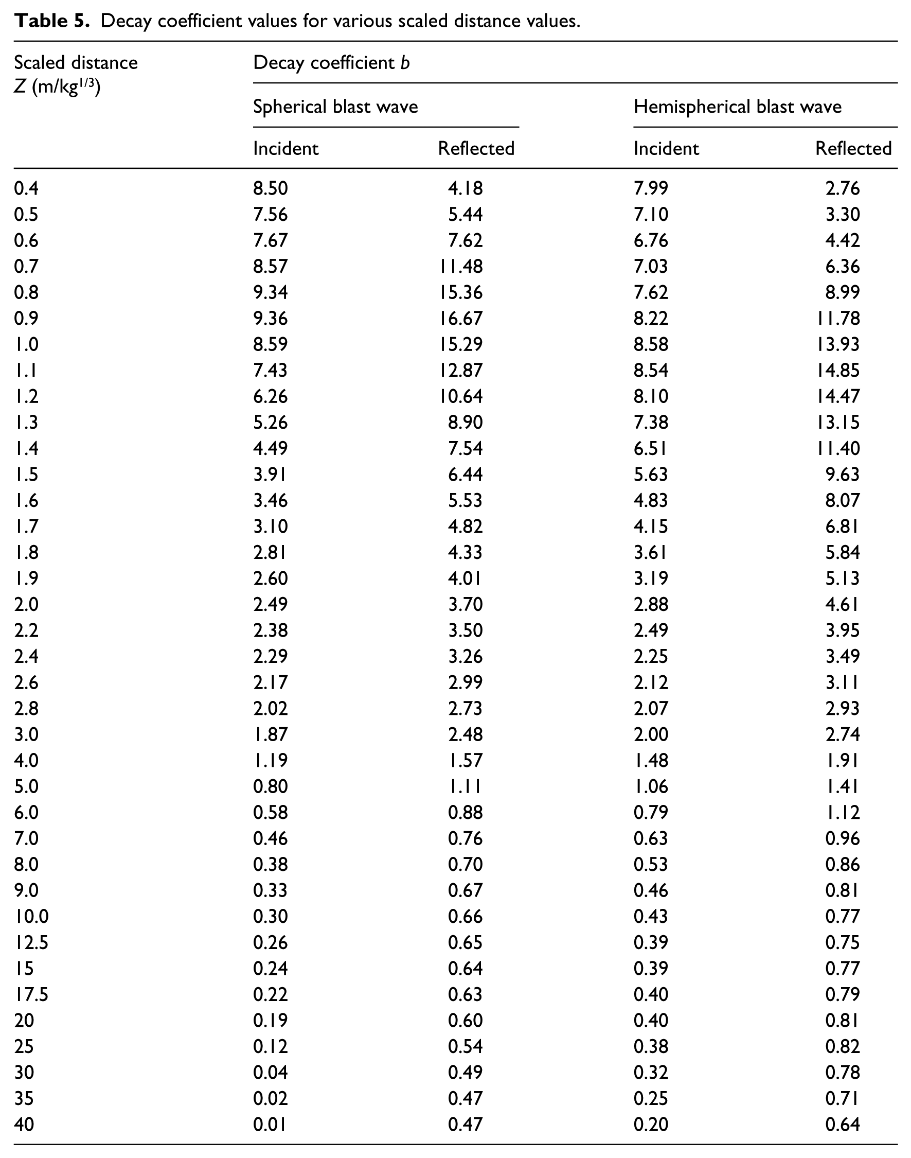
Scaled distanceZ (m/kg^1/3)	Decay coefficient b
Scaled distanceZ (m/kg^1/3)	Spherical blast wave		Hemispherical blast wave
	Incident	Reflected	Incident	Reflected
0.4	8.50	4.18	7.99	2.76
0.5	7.56	5.44	7.10	3.30
0.6	7.67	7.62	6.76	4.42
0.7	8.57	11.48	7.03	6.36
0.8	9.34	15.36	7.62	8.99
0.9	9.36	16.67	8.22	11.78
1.0	8.59	15.29	8.58	13.93
1.1	7.43	12.87	8.54	14.85
1.2	6.26	10.64	8.10	14.47
1.3	5.26	8.90	7.38	13.15
1.4	4.49	7.54	6.51	11.40
1.5	3.91	6.44	5.63	9.63
1.6	3.46	5.53	4.83	8.07
1.7	3.10	4.82	4.15	6.81
1.8	2.81	4.33	3.61	5.84
1.9	2.60	4.01	3.19	5.13
2.0	2.49	3.70	2.88	4.61
2.2	2.38	3.50	2.49	3.95
2.4	2.29	3.26	2.25	3.49
2.6	2.17	2.99	2.12	3.11
2.8	2.02	2.73	2.07	2.93
3.0	1.87	2.48	2.00	2.74
4.0	1.19	1.57	1.48	1.91
5.0	0.80	1.11	1.06	1.41
6.0	0.58	0.88	0.79	1.12
7.0	0.46	0.76	0.63	0.96
8.0	0.38	0.70	0.53	0.86
9.0	0.33	0.67	0.46	0.81
10.0	0.30	0.66	0.43	0.77
12.5	0.26	0.65	0.39	0.75
15	0.24	0.64	0.39	0.77
17.5	0.22	0.63	0.40	0.79
20	0.19	0.60	0.40	0.81
25	0.12	0.54	0.38	0.82
30	0.04	0.49	0.32	0.78
35	0.02	0.47	0.25	0.71
40	0.01	0.47	0.20	0.64

Declaration of conflicting interests

The author(s) declared no potential conflicts of interest with respect to the research, authorship, and/or publication of this article.

Funding

The author(s) received no financial support for the research, authorship, and/or publication of this article.

References

Baker

(1973) Explosions in Air. Austin, TX; London: University of Texas Press.

Baker

Cox

Westine

. (1983) Explosion Hazards and Evaluation. Amsterdam: Elsevier.

Bogosian

Ferritto

Shi

(2002) Measuring uncertainty and conservatism in simplified blast models. In: 30th explosives safety seminar, Atlanta, GA, 13–15 August.

Borenstein

Benaroya

(2009) Sensitivity analysis of blast loading parameters and their trends as uncertainty increases. Journal of Sound and Vibration 321: 762–785.

Borgers

Vantomme

(2008) Improving the accuracy of blast parameters using a new Friedlander curvature α. In: Department of Defence (DOD) explosives safety seminar, Palm Springs, CA, 12–14 August.

Brode

(1955) Numerical solution of spherical blast waves. Journal of Applied Physics: American Institute of Physics 26(6): 766–775.

Brode

(1956) Point source explosion in air. U.S. Air Force: Project RAND, AD 133030, 3 December. Santa Monica, CA: RAND Corporation. Available at: https://www.rand.org/content/dam/rand/pubs/research_memoranda/2008/RM1824.pdf

Brode

(1968) Review of nuclear weapons effects. Annual Review of Nuclear Science 18: 153–202.

Campidelli

Tait

El-Dakhakhni

. (2015) Inference of blast wavefront parameter uncertainty for probabilistic risk assessment. Journal of Structural Engineering 141(12): 04015062.

10.

Chock

Kapania

(2001) Review of two methods for calculating explosive Air blast. The Shock and Vibration Digest 33(2): 91–102.

11.

Cranz

(1926) Lehrbuch del Ballistik. Berlin: Springer.

12.

Dharaneepathy

Kwshava Rao

Santhakumar

(2006) Critical distance for blast resistant design. International Journal of Impact Engineering 32(12): 2032–2047.

13.

Esparza

(1986) Blast measurements and equivalency for spherical charges at small scaled distances. International Journal of Impact Engineering 4: 23–40.

14.

EUROPLEXUS (2013) User’s manual. Available at: http://europlexus.jrc.ec.europa.eu

15.

Goel

Matsagar

Gupta

. (2012) An abridged review of blast wave parameters. Defence Science Journal 62(5): 300–306.

16.

Goodman

(1960) Compiled Free-Air Blast Data on Bare Spherical Pentolite. AD No. 235275. Aberdeen Proving Ground, MD: U.S. Army Ballistic Research Laboratory.

17.

Henrych

(1979) The Dynamics of Explosions and Its Use. Amsterdam: Elsevier.

18.

Hopkinson

(1915) British Ordnance board minutes No. 13565. p. 220.

19.

International Ammunition Technical Guideline (IATG) (2011) Formulae for Ammunition Management 01.80. New York: United Nations.

20.

Ismail

Murray

(1993) Study of the blast wave parameters from small scale explosions. Propellants, Explosives, Pyrotechnics 18: 11–17.

21.

Karlos

Solomos

(2013) Calculation of blast loads for application to structural components. JRC Technical Report, EUR 26456EN, December. Luxembourg: European Union.

22.

Karlos

Solomos

(2016) Analysis of blast parameters in the near-field for spherical free-air explosions. JRC Technical Report, EUR 27823EN, December. Luxembourg: European Union.

23.

Kingery

(1966) Air Blast Parameters versus Distance for Hemispherical TNT Surface Bursts. Aberdeen Proving Ground, MD: Ballistic Research Laboratories.

24.

Kingery

Bulmash

(1984) Technical report ARBRL-TR-02555: air blast parameters from TNT spherical air burst and hemispherical burst. AD-B082 713, Aberdeen Proving Ground, MD: U.S. Army Ballistic Research Laboratory.

25.

Kingery

Coulter

(1983) Reflected Overpressure Impulse on a Finite Structures. Aberdeen Proving Ground, Maryland, MD: Ballistic Research Laboratory.

26.

Kinney

Graham

(1985) Explosive Shocks in the Air. Berlin: Springer.

27.

Krauthammer

(2008) Modern Protective Structures. Boca Raton, FL: CRC Press.

28.

Lam

Mendis

Ngo

(2004) Response spectrum solutions for blast loading. Electronic Journal of Structural Engineering 4: 28–44.

29.

Larcher

(2007) Simulation of the effects of an air blast wave. JRC Technical Report, EUR 41337EN, January. Luxembourg: European Union.

30.

Mills

(1987) The design of concrete structures to resist explosions and weapon effects. In: Proceedings of the 1st international conference on concrete for hazard protections, Edinburg, 27–30 September, pp. 61–73. Paris: Concrete Society.

31.

Naumyenko

Petroskyi

(1956) The shock wave of a nuclear explosion. BOEH, CCCP.

32.

Netherton

Stewart

(2010) Blast load variability and accuracy of blast load prediction models. International Journal of Protective Structure 1(4): 543–570.

33.

Ngo

Lumantarna

Whittaker

. (2015) Quantification of the blast-loading parameters of large-scale explosions. Journal of Structural Engineering: American Society of Civil Engineers 141: 04015009.

34.

Rigby

Fay

Tyas

. (2015a) Angle of incidence effects on far-field positive and negative phase blast parameters. International Journal of Protective Structures 6(1): 23–42.

35.

Rigby

Tyas

Bennett

. (2014a) The negative phase of the blast load. International Journal of Protective Structures 5(1): 1–20.

36.

Rigby

Tyas

Clarke

. (2015b) Observations from preliminary experiments on spatial and temporal pressure measurements from near-field free air explosions. International Journal of Protective Structures 6(2): 175–190.

37.

Rigby

Tyas

Fay

. (2014b) Validation of semi-empirical blast pressure predictions for far field explosions—Is there inherent variability in blast wave parameters? In: 6th international conference on protection of structures against hazards, Tianjin, China, 16–17 October.

38.

Sadovsky

(2004) Mechanical effects of air shock waves from explosions according to experiments. In: Physics of explosions: symposium No.4. Moscow: AN SSR.

39.

Shin

Whittaker

Cormie

(2015) Incident and normally reflected overpressure and impulse for detonations of spherical high explosives in free air. Journal of Structural Engineering 141: 04015057.

40.

Smith

Hetherington

(1994) Blast and Ballistic Loading of Structures. London: Butterworth-Heinemann Ltd.

41.

Teich

(2012) Interaktionen von Explosionen mit flexiblen Strukturen. PhD Thesis, Universität der Bundeswehr München, Munich.

42.

Teich

Gebbeken

(2010) The influence of the underpressure phase on the dynamic response of structures subjected to blast loads. International Journal of Protective Structures 1(2): 219–234.

43.

Twisdale

Sues

Favelle

(1993) Reliability-Based Analysis and Design Methods for Reinforced Concrete Protective Structures. Panama City, FL: Engineering Research Division, Air Force Civil Engineering Support Agency.

44.

Unified Facilities Criteria (2008) UFC 3-340-02 Structures to Resist the Effects of Accidental Explosions. Washington, DC: U.S. Army Corps of Engineers, Naval Facilities Engineering Command, Air Force Civil Engineer Support Agency.

45.

Department of the Army, the Navy and the Air Force (1990) Structures to resist the effects of accidental explosions. Army Technical Manual 5-1300. Washington, DC: Navy Publication NAVFAC P-397, Air Force Manual AFM 88-22.

46.

Hao

(2005) Modeling of simultaneous ground shock and airblast pressure on nearby structures from surface explosions. International Journal Of Impact Engineering 31(6): 699–717.

Analysis of the blast wave decay coefficient using the Kingery–Bulmash data

Abstract

Keywords

Introduction

Blast wave characteristics

Blast pressure decay coefficient formulations

Decay coefficient using the Kingery–Bulmash parameters

Free-air bursts

Incident blast wave

Reflected blast wave

Surface bursts

Decay coefficient comparison

Assessment of derived expressions

Comparison with experimental data

Sensitivity analysis and trends

Conclusion

Footnotes

Appendix 1

Declaration of conflicting interests

Funding

References