Sage Journals: Discover world-class research

Abstract

The current study used longitudinal panel data from the National Longitudinal Survey of Youth 1979 (NLSY79; n = 7,064) and National Longitudinal Survey of Young Adults (NLSY-YA; n = 2,985) to examine whether political party affiliation was related to residential mobility between rural regions, urban regions, and major cities in the United States. Over a follow-up of 4–6 years, stronger Republican affiliation was associated with lower probability of moving from rural regions to major cities (relative risk [RR] = 0.71, confidence interval [CI] = [0.54, 0.93]) and higher probability of moving away from major cities to urban or rural regions (RR = 1.17, CI = [1.03, 1.33]). The empirical correlation between party affiliation and urban–rural residence was r = −0.15 [−0.17, −0.13]. Simulated data based on the regression models produced a correlation of r = −0.06 [−0.10, −0.03], suggesting that selective residential mobility could account almost half of the empirically observed association between party affiliation and urban–rural residence.

Keywords

attitudes political psychology values

Individuals living in urban and rural regions of the United States differ from each other in their political attitudes (Gimpel et al., 2019; Scala & Johnson, 2017). Liberal Democrats are most likely to live in urban areas and metropolitan centers, while conservative Republicans tend to live in more rural regions. This urban–rural divide has widened over time: Data from the Pew Research Center shows that the proportion of Democrats in urban counties increased from 55% to 62% between 1998 and 2017 (Parker et al., 2018). During the same period, the proportion of Republicans in urban counties decreased from 37% to 31%. It is important to understand the geographic evolution of political orientations as geography is one of the components contributing to the overall political polarization in the United States (Motyl, 2016; Wilkinson, 2018).

Selective residential mobility is one possible explanation for the development of urban–rural differences in political attitudes (Motyl, 2016; Wilkinson, 2018). People may actively seek, or passively drift, to neighborhoods that are populated by like-minded others; many observable neighborhood characteristics, such as the types of cars or number of churches, can provide cues about the residents’ political leanings that people notice when selecting neighborhoods (Gebru et al., 2017). Even if people did not specifically seek for neighbors with similar political views, individuals with different political attitudes tend to prefer different kinds of neighborhoods (Motyl et al., 2019), which may steer political segregation (Carlson & Gimpel, 2019). Personality traits have also been shown to cluster geographically (Rentfrow & Jokela, 2016; Rentfrow et al., 2015) and to predict selective residential mobility across urban and rural regions (Butikofer & Peri, 2017; Campbell, 2019; Jokela, 2020). Given that political attitudes are correlated with personality traits (Gerber et al., 2010), selective residential mobility associated with political party affiliation seems plausible.

The hypothesis of sorting into like-minded communities has received much attention in academic research and public discussions (Abrams & Fiorina, 2012; Bishop, 2009; Rodden, 2019; Rohla et al., 2018; Wilkinson, 2018). But selective mobility cannot be taken as the only explanation for the evolution of urban–rural differences. Living in an urban versus rural community might differently mold people’s political views in response to political views of their neighborhood peers (Johnston et al., 2004; Lazer et al., 2010) or other neighborhood characteristics that correlate with political attitudes. Changing political geographies could also be driven by third variables that influence migration or subsequent development of political attitudes (e.g., lifestyle factors, family structure) or by changes in the policies pursued by political parties that appeal differently to urban versus rural voters.

There seems to no studies that would have used individual-level data to directly assess whether political party identification is related to subsequent residential mobility between urban and rural neighborhoods. The available longitudinal evidence for the sorting hypothesis is largely based on regional changes in voting results (Scala & Johnson, 2017) or repeated cross-sectional surveys (Parker et al., 2018). In the absence of individual-level data from longitudinal panel studies, it is difficult to evaluate whether and how strongly political party affiliation actually predicts the mobility of individuals between urban and rural regions.

The current study used data from two longitudinal studies to examine whether political party affiliation assessed in 2008 predicted the participants’ residential mobility across rural areas, urban areas, and major cities of the United States over 4–6 years. The longitudinal panel data made it possible to directly test whether people with different political leanings have different probabilities of migrating between urban and rural areas. I hypothesized that people who support Democrats would have higher rates of rural-to-urban migration whereas support for Republicans would be related to urban-to-rural migration. In addition to the empirical assessment of these associations (Study 1), I fitted a simple simulation model to assess how large the urban–rural difference in political party affiliation would be expected to grow if the estimated associations would hold over time and whether the selective residential mobility would be sufficient to account for the empirically observed correlation between urban–rural residence and political party affiliation (Study 2).

Study 1: Empirical Analysis

Method

Participants were from the National Longitudinal Survey of Youth started in 1979 (NLSY79) and the National Longitudinal Survey of Young Adults (NLSY-YA) that started in 1986 to recruit the children of the women participants of the original NLSY79. For the present analysis, study baseline was the year 2008 for both cohorts when the political party affiliation questions were included in the surveys, and the participants were followed between 2008 and 2014 in NLSY79 (n = 24,951 person-observations of 7,064 participants) and between 2008 and 2012 in NLSY-YA (n = 5,137 person-observations of 2,985 persons). The sample size was determined based on the number of participants of the two cohort studies who had data on the study variables. The NLSY data are publicly available at https://www.nlsinfo.org.

The NLSY participants’ residential location has been recorded with two indicators: urban–rural residence (1 = urban, 2 = rural) and metropolitan statistical area (MSA) residence (1 = not in MSA, 2 = in MSA but not in central city, 3 = MSA, central city). The urban/rural variable is based on the definition of the U.S. Census Bureau by which urban areas are densely settled cores of census tracts and/or census blocks that meet minimum population density requirements: Urban areas can be urbanized areas (50,000 or more people) or urban clusters (between 2,500 and 50,000 people). All other locations are considered rural. An MSA refers to a wider geographical region that contains a large urban core area and adjacent communities that have a high degree of integration with that core. An MSA consists of one or more counties that contain a city of 50,000 or more inhabitants or contain an urbanized area and have a total population of at least 100,000 (75,000 in New England). The largest city in each MSA is designated as a central city, and additional cities of the MSA can qualify for this designation if specified requirements are met concerning population size and commuting patterns. Based on these two variables, the residential location of the participants was coded as 1 = rural (rural and/or not in MSA), 2 = urban (urban and/or in MSA but not in central city), and 3 = major city (MSA, in central city). Thus, I refer to “major cities” instead of “central cities” because the term “major city” better conveys the nature of the location.

Political party affiliation was assessed by first asking the participants “Generally speaking, do you usually think of yourself as a Democrat, a Republican, an Independent, or what?” (1 = Democrat, 2 = Republican, 3 = Independent, 4 = Other party, 5 = no preference; the order of Democrat and Republican options in the question was alternated across interviews). If the participant responded either Democrat or Republican, a follow-up question asked “A strong (Democrat/Republican) or a not very strong (Democrat/Republican)?” If the participant reported supporting some other party, the participant was first asked which party and then “Do you think of yourself as closer to the Democratic Party, closer to the Republican Party, or equally close to both?” (1 = closer to Republican Party, 2 = closer to Democratic Party, 3 = equally close, 4 = neither; the order of Democratic and Republican options was alternated across interviews). Based on these three questions, it was possible to derive a seven-category variable describing a Democrat–Republican continuum: 1 = strong Democrat, 2 = not very strong Democrat, 3 = closer to Democratic Party, 4 = Independent or Other party, equally close to Democratic and Republican parties, or neither, 5 = closer to Republican Party, 6 = not very strong Republican, and 7 = strong Republican. This variable was used as a continuous regressor in the statistical analysis. To facilitate the interpretation of the relative risk ratios of the regression models, I divided the Party Affiliation Scale by 4 so that a one-unit difference indicated a difference between moderate Democrats (2) and moderate Republicans (6).

Additional sociodemographic covariates included marital status (0 = not married, 1 = married), highest grade completed (1 = high school or less, 2 = 1–2 years of college, 3 = 3 or more years of college), income decile, employment status (0 = working, 1 = not working), student status (0 = not studying, 1 = studying; only included in the NLSY-YA), and family size.

Associations between political party affiliation and residential mobility were assessed with multinomial logistic regression models predicting the location in the next study wave, fitted separately by baseline residence and cohort (i.e., three multinomial logistic regression models for both cohorts, fitted separately for those living in rural areas, urban areas, and major cities). Each participant could contribute more than one person-observation in the data set (up to three person-observations for follow-ups between 2008 and 2010, 2010 and 2012, and 2012 and 2014 in NLSY79 and up to two person-observations for follow-ups between 2008 and 2010 and 2010 and 2012 in NLSY-YA), so the standard errors were estimated using robust estimators with participant as the clustering variable. Moreover, participants of the NLSY79 were parents of the NLSY-YA participants, so not all the observations were independent of each other, which might have led to underestimation of standard errors. As a sensitivity analysis, I combined the cohorts into a single data set and fitted the multinomial logistic regression models with the family identification number as the clustering variable for parents and all their children when estimating standard errors with the robust estimation method. The results from the two cohorts were pooled together with fixed-effect meta-analysis. In the NLSY-YA, some of the participants were still living with their parents, and these person-observations were excluded from the analysis (n = 2,260 person-observations) because presumably they were not making the residential mobility choices of the household.

Results

Table 1 reports the descriptive statistics of the two cohort studies. Figure 1 shows the associations of party affiliation with subsequent residential mobility between study waves, which were quite similar in NLSY79 and NLSY-YA. Stronger Republican Party affiliation was associated with lower probability of moving from rural regions to major cities (relative risk [RR] = 0.71 per a 4-point difference in the Party Affiliation Scale, confidence interval [CI] = [0.54, 0.93]) and higher probability of moving away from major cities to urban regions (RR = 1.18, CI = [1.02, 1.37]) or rural regions (RR = 1.19, CI = [0.92, 1.55]). The latter association was not statistically significant, but the effect size was essentially the same as for the former, and the averaged effect size for moving from major cities to either urban or rural regions was RR = 1.17, CI = [1.03, 1.33].

Table 1.

Descriptive Statistics.

Covariate	NLSY79	NLSY-YA
Gender
Men	48.2 (3,408)	44.5 (1,329)
Women	51.8 (3,656)	55.5 (1,656)
Residence
Rural	28.3 (1,996)	25.1 (748)
Urban	53.9 (3,805)	42.7 (1,274)
Major city	40.7 (2,877)	49.6 (1,479)
Party affiliation
Strong Democrat	28.3 (2,002)	19.9 (594)
Moderate Democrat	16.6 (1,172)	23.2 (691)
Leaning Democrat	7.7 (542)	8.1 (242)
Neither	19.5 (1,379)	27.4 (819)
Leaning Republican	5.1 (363)	3.3 (98)
Moderate Republican	11.1 (785)	11.5 (342)
Strong Republican	11.6 (821)	6.7 (199)
Ethnic group
White, non-Hispanic	50.6 (3,572)	45.4 (1,355)
Hispanic	18.3 (1,293)	19.4 (579)
Black	31.1 (2,199)	35.2 (1,051)
Age at baseline (years)^a	49.9 (3.4)	26.1 (3.3)
n (person-observations)	24,951	5,137
n (persons)	7,064	2,985

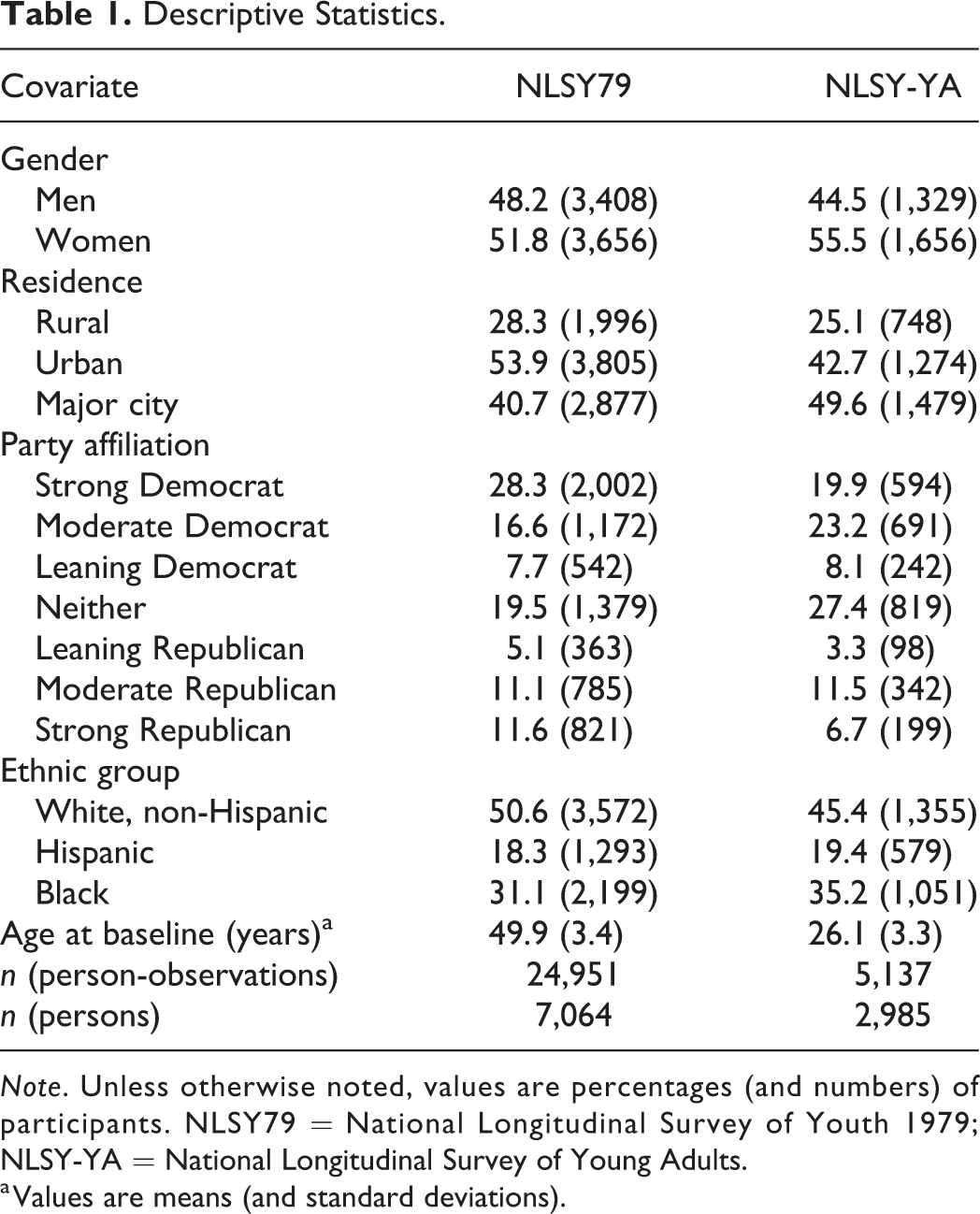
Note. Unless otherwise noted, values are percentages (and numbers) of participants. NLSY79 = National Longitudinal Survey of Youth 1979; NLSY-YA = National Longitudinal Survey of Young Adults.

^a Values are means (and standard deviations).

Figure 1.

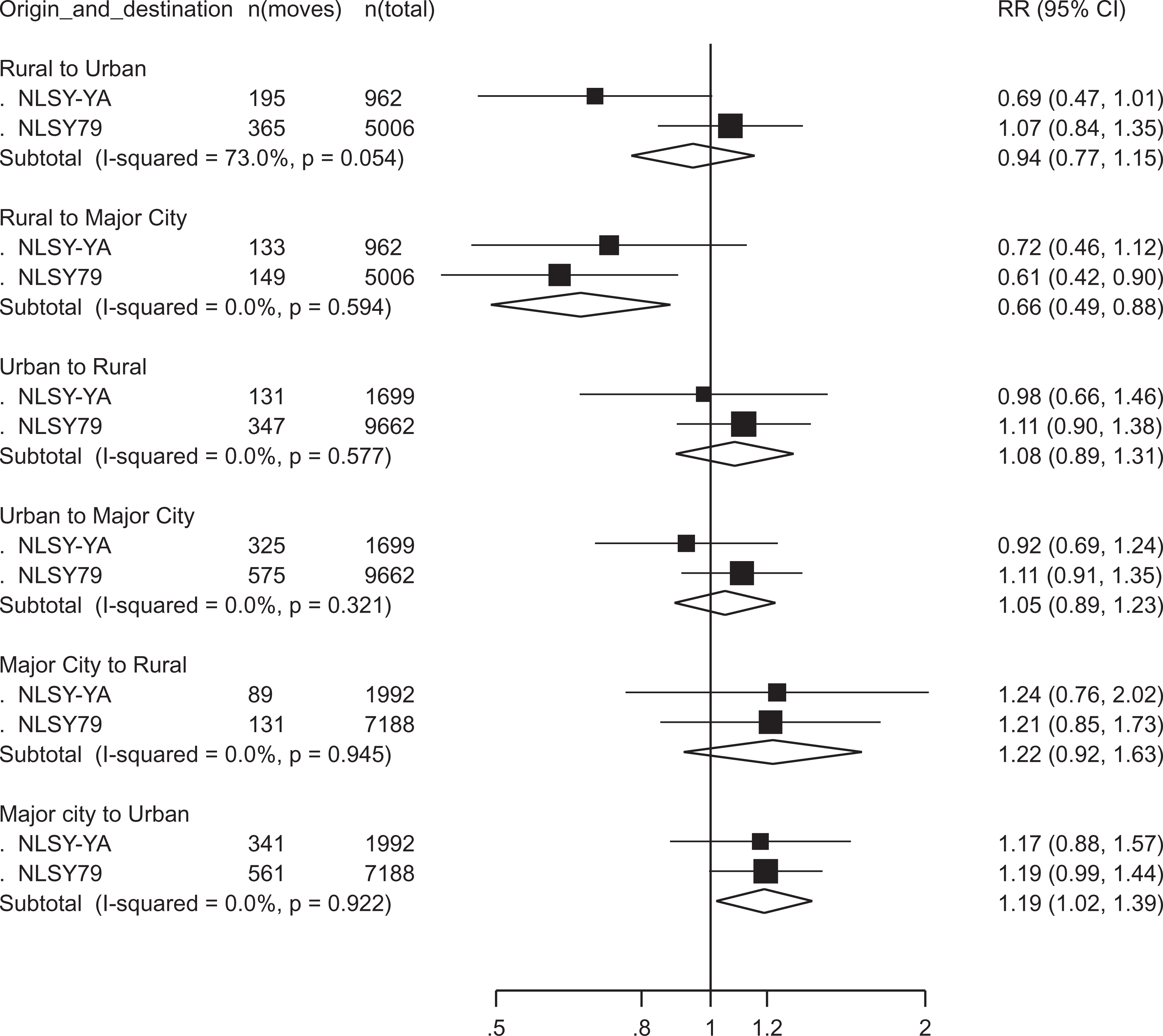
Residential mobility between major cities, urban areas, and rural areas associated with political party affiliation. Note. Values are relative risks of moving between locations associated with a 4-point difference in the Party Affiliation Scale (range 1–7, higher values indicating stronger Republican support); the 4-point difference was equal to a comparison between moderate Republicans versus moderate Democrats. Reference group was nonmovers. Three multinomial logistic regression models were fitted for both cohorts (separately by baseline residence). The associations were adjusted for age (linear and quadratic), gender, and race/ethnicity. NLSY79 = National Longitudinal Study 1979, NLSY-YA = National Longitudinal Study Young Adults, RR = relative risk, CI = confidence interval, I ² = heterogeneity of the pooled estimate.

These associations remained largely unchanged when adjusted for the sociodemographic factors: RR = 0.66 (0.49, 0.88) for rural to major city, RR = 1.19 (1.02, 1.39) for major city to urban, and RR = 1.22 (0.92, 1.63) for major city to rural (Supplementary Figure S1). The conclusions also remained largely the same when the data from the two cohorts were pooled together, and standard errors were estimated using family (instead of person) as the clustering variable, which took into account the nonindependence of the NLSY79 and NLSY-YA participants (Supplementary Figure S2).

Study 2: Simulation

The regression models above yielded relative risk ratios of for the associations between political party affiliation and urban–rural mobility. These estimates did not yet tell what the consequences would be for urban–rural differences in the long run if the estimates were true; even small effect sizes may accumulate to meaningful population-level patterns (Götz et al., 2021). In order to estimate the development of urban–rural differences based on selective residential mobility, I ran a simple simulation model in which a cohort of 20-year-olds were randomly assigned to locations (rural, urban, and major city), and then they were allowed to move based on the probabilities derived from the regression models estimated in the empirical analysis, taking into account party affiliation, age, and current location. The simulation thus illustrated how strong an association between urban–rural residence and political party affiliation would develop over time based on the mobility estimates and how the simulated associations compared with the associations observed in the empirical data.

Method

The simulations were based on a modified data set that mimicked the U.S. general population. All individuals started the simulation at age 20, with gender set to 1.5 for all individuals (to represent equal numbers of women and men but not allowing gender to predict mobility), and ethnic groups of Hispanic and African Americans were both given values of 0.15. Political party affiliation was randomly assigned following the approximate national distribution reported by the Pew Research Center (2019) survey data from the 2010s (15% strong Democrats, 15% moderate Democrats, 20% leaning toward Democrats, 10% neither, 15% leaning toward Republicans, 12.5% moderate Republicans, and 12.5% strong Republicans; the Pew survey did not have separate categories for strong and moderate support, so I split the original Democrat and Republican categories into half for the purpose of the simulation to have a 7-point scale). Baseline urban–rural residence was randomly assigned for all individuals from a distribution of the original proportions (20% rural, 45% urban, and 35% major cities).

The simulation progressed in 2-year steps over which the individuals could move across major cities, urban regions, and rural regions based on the probabilities determined from the multinomial regression models, taking into account their party affiliation, current residential location, and increasing age. The simulation was run for 40 years between ages 20 and 60. The results were plotted as the proportions of Democrats and Republicans (the sum of strong, moderate, and leaning categories, which were treated as separate categories in the simulation but combined for the illustration of the results) in rural regions, urban regions, and major cities. To estimate confidence intervals, I fitted the simulations 200 times, each time using a bootstrapped sample to estimate the multinomial logistic regression models to take into account uncertainty in the estimated coefficients; the simulations did not consider the statistical significance of the coefficients when calculating the predicted probabilities of moving.

Results

Between ages 20 and 40, the simulated proportion of Democrats increased from 50% to 53% in major cities, decreased from 50% to 49% in urban regions, and decreased from 50% to 47% in rural regions (Figure 2). The proportion of Republicans decreased from 40% to 37% in major cities, increased from 40% to 42% in urban regions, and increased from 40% to 43% in rural regions. These differences changed only little between ages 40 and 60 (Table 2) as the probability of moving decreased with age.

Figure 2.

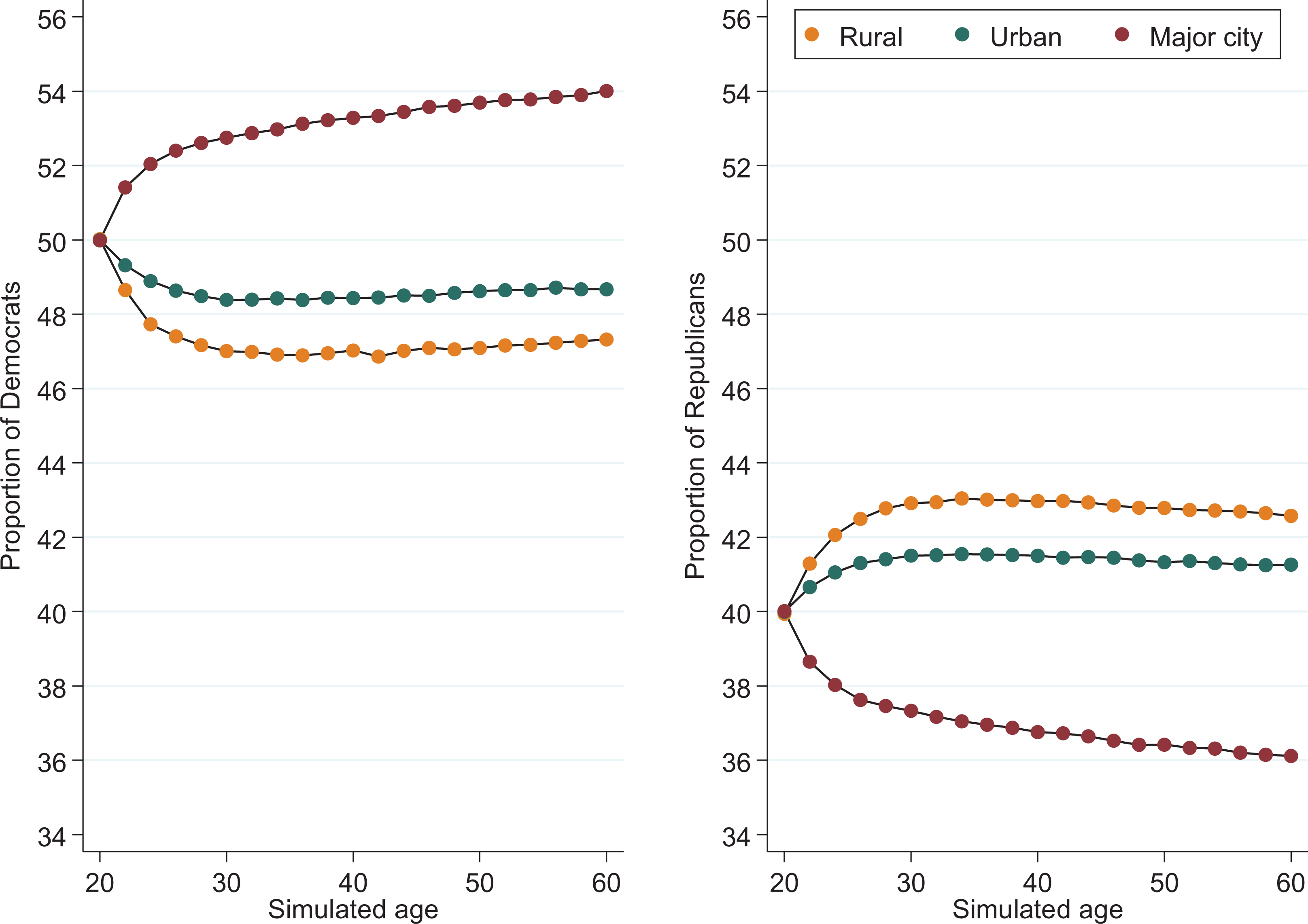
Simulated proportions (%) of Democrats (left) and Republicans (right) in rural regions, urban region, and major cities by age. Note. Simulations assumed that the population consisted of 50% Democrats and 40% Republicans whose baseline residence was randomly assigned (10% of the population supported neither Democrats nor Republicans). The individuals were then allowed to move between locations based on the regression model estimates taking into account party affiliation, age, and current location.

Table 2.

Simulated Percentages of Democrats and Republicans in Rural Regions, Urban Regions, and Major Cities at Ages 20, 40, and 60.

Party affiliation	Age	Rural	Urban	Major City
Democrats	20	50.0 [49.3, 50.7]	50.0 [49.4, 50.4]	50.0 [49.5, 50.5]
	40	46.8 [43.9, 49.8]	48.5 [46.7, 50.0]	53.3 [51.3, 55.7]
	60	47.0 [44.3, 50.2]	48.8 [46.8, 50.2]	53.9 [51.5, 57.0]
Republicans	20	40.0 [39.3, 40.8]	40.0 [39.6, 40.5]	40.0 [39.4, 40.6]
	50	43.1 [40.3, 46.1]	41.5 [39.9, 43.3]	36.8 [34.6, 38.7]
	60	42.9 [39.8, 45.3]	41.2 [39.7, 43.1]	36.1 [33.3, 38.5]

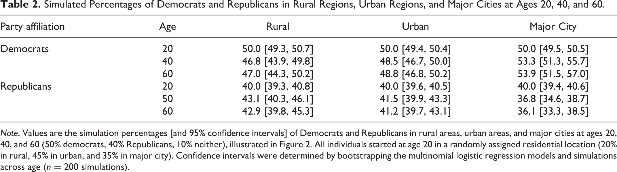
Note. Values are the simulation percentages [and 95% confidence intervals] of Democrats and Republicans in rural areas, urban areas, and major cities at ages 20, 40, and 60 (50% democrats, 40% Republicans, 10% neither), illustrated in Figure 2. All individuals started at age 20 in a randomly assigned residential location (20% in rural, 45% in urban, and 35% in major city). Confidence intervals were determined by bootstrapping the multinomial logistic regression models and simulations across age (n = 200 simulations).

The empirical correlation between party affiliation and urban–rural residence at baseline in 2008 was r = −0.15 [−0.17, −0.13]. The simulated selective migration patterns illustrated in Figure 2 led to an individual-level correlation of r = −0.06 [−0.10, −0.03] between urban–rural residence and political party affiliation (Figure 3), suggesting that selective mobility process could account for slightly less than half of the empirical correlation. This difference between the empirical and simulated correlation was not due to the difference between party affiliation distributions in the empirical and simulated data: The simulated correlation was the same (r = −0.06, CI = [−0.03, −0.10]) when the simulation was run using the empirical party affiliation distribution (Table 1) instead of the party affiliation distribution based on the Pew survey data.

Figure 3.

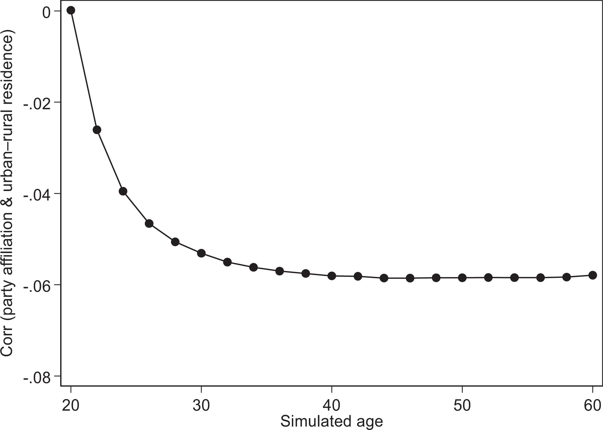
Simulated correlations between political party affiliation and urban–rural residence at different ages based on the simulated data shown in Figure 2.

Discussion

The current study provides direct longitudinal evidence on how political party affiliation of individuals predicts their subsequent residential mobility across urban and rural regions of the United States. Compared to those supporting Democrats, individuals supporting Republicans were less likely to move from rural areas to major cities and were more likely to move away from major cities. Simple simulation models based on the regression models indicated that, between ages 20 and 40, selective residential mobility would have widened the political divide by 6 percentage points in major cities (from 50% Democrats vs. 40% Republicans to 53% Democrats vs. 37% Republicans) and by 6 percentage points in rural areas (from 50% Democrats vs. 40% Republicans to 47% Democrats vs. 43% Republicans).

Individuals with conservative versus liberal political views have different neighborhood preferences (Gimpel & Hui, 2017; Motyl, 2016; Motyl et al., 2019), and many of these preferences correlate with the urban–rural continuum. For example, when more than 3,000 U.S. adults were asked to select 10 of their most important characteristics for their ideal community, liberal participants were more likely than conservative to select ethnic diversity, many atheists, well-educated residents, good public transportation, lots of vegetarian restaurants, and urban community. Conservative participants were more likely than liberals to select characteristics such as wealthy community, friendly neighbors, patriotic and religious community, many churches, family-friendly, and rural community (Motyl et al., 2019). People also associate many neighborhood characteristics with politics, which allows their own political views to influence selective residential mobility based on political and neighborhood preferences (Gimpel & Hui, 2015). In the present study, the selective residential mobility patterns associated with party affiliation did not seem to be mere side effects of sociodemographic factors, as the results remained almost unchanged when adjusted for education, employment status, income, marital status, and household size.

In the simulated models, selective residential mobility led to a correlation of −0.06 between party affiliation and urban–rural residence, which was less than half of the empirical correlation of −0.15 in the NLSY cohorts. Given that residential mobility decreased considerably after age 40, most of the correlation between urban–rural residence and political affiliation emerged between ages 20 and 40. The difference between the simulated and observed correlation suggests that selective residential mobility alone may not be sufficient to account for the urban–rural political difference completely and that other processes may be involved. For example, people’s political attitudes may be influenced by the political attitudes of their local peers (Huckfeldt et al., 2013) or the environmental characteristics of urban versus rural neighborhoods. However, it must be emphasized that the simulation was very simple and did not consider any possible compounding or long-term effects of selective residential mobility, which may have underestimated the contribution of selective mobility on urban–rural differences. For example, spouses resemble each other in political attitudes (Alford et al., 2011), which might increase the overall geographic clustering of party affiliation beyond that estimated for single individuals. Intergenerational transmission of party affiliation from parents to offspring (Kandler et al., 2012) could also compound the effects of parents’ selective mobility over the long term.

Three limitations need to be emphasized. First, the analysis was limited by a rather crude urban–rural residence indicator. The Census-defined category of urban areas in the United States includes all the sufficiently densely populated locations, ranging from small towns to large cities. Rural areas are defined simply as not being urban. More detailed indicators of the urban–rural continuum would be useful to characterize the selective mobility patterns with better geographic resolution. In the present analysis, selective residential mobility related to political affiliation was observed mainly between major cities versus other locations (i.e., rural or other urban regions). This is in line with population-level results showing that the association between population density and votes for Democrats is nonlinear, that is, particularly strong for the most densely populated cities (Rodden, 2019; Wilkinson, 2018).

Second, political orientation was assessed only with political party affiliation. It is unknown whether the selective mobility patterns are driven by global ideological views or by more specific social or political attitudes that may vary within political party affiliations (Hanel et al., 2019). Future studies need to assess political orientation with more detailed measures. Third, the longitudinal data demonstrated that selective residential mobility was associated with political party affiliation, but these data cannot determine whether selective residential mobility is caused by political attitudes; there may be some other characteristics that determine people’s mobility decisions and correlate with political attitudes that were not assessed in the present study. However, political attitudes would still get geographically sorted even if they were not the causal factors of migration decisions and merely correlated with the causal factors. Future studies should assess whether factors such as lifestyle preferences, neighborhood perceptions, or personality traits might help to explain the selective migration associated with political party affiliation.

In summary, people’s political party affiliation was related to selective urban–rural residential mobility in the United States over a follow-up of 4–6 years so that people supporting Republicans were less likely to move to major cities and were more likely to move away from major cities compared to people supporting Democrats. Results from a simple simulation model suggested that selective residential mobility could explain slightly less than half of the urban–rural difference in political party affiliation, indicating that other mechanisms are likely to be involved in creating urban–rural political differences (e.g., neighborhood influence on the development of political views). Studies with more fine-grained measures of political attitudes and neighborhoods, both assessed repeatedly over many years, are needed to fully describe the development of urban–rural differences in political orientation.

Supplemental Material

Supplemental Material, sj-pdf-1-spp-10.1177_1948550621994000 - Urban–Rural Residential Mobility Associated With Political Party Affiliation: The U.S. National Longitudinal Surveys of Youth and Young Adults

Supplemental Material, sj-pdf-1-spp-10.1177_1948550621994000 for Urban–Rural Residential Mobility Associated With Political Party Affiliation: The U.S. National Longitudinal Surveys of Youth and Young Adults by Markus Jokela in Social Psychological and Personality Science

Footnotes

Declaration of Conflicting Interests

The author(s) declared no potential conflicts of interest with respect to the research, authorship, and/or publication of this article.

Funding

The author(s) received no financial support for the research, authorship, and/or publication of this article.

ORCID iD

Markus Jokela

Supplemental Material

The supplemental material is available in the online version of the article.

Author Biography

Markus Jokela is a Professor of Psychology. His research explores the connections between individual differences and population outcomes.

Handling Editor: Peter Rentfrow

References

Abrams

S. J.

Fiorina

M. P.

(2012). “The big sort” that wasn’t: A skeptical reexamination. Political Science & Politics, 45(02), 203–210. https://doi.org/10.1017/S1049096512000017

Alford

J. R.

Hatemi

P. K.

Hibbing

J. R.

Martin

N. G.

Eaves

L. J.

(2011). The politics of mate choice. The Journal of Politics, 73(2), 362–379. https://doi.org/doi:10.1017/S0022381611000016

Bishop

(2009). The big sort: Why the clustering of like-minded America is tearing us apart. Mariner Books.

Butikofer

Peri

(2017). The effects of cognitive and noncognitive skills on migration decisions. SSRN Electronic Journal. https://doi.org/10.2139/ssrn.3041090

Campbell

(2019). Dispositional traits and internal migration: Personality as a predictor of migration in Australia. Journal of Research in Personality, 78, 262–267. https://doi.org/10.1016/j.jrp.2018.12.009

Carlson

Gimpel

J. G.

(2019). Political implications of residential mobility and stasis on the partisan balance of locales. Political Geography, 71(February), 103–114. https://doi.org/10.1016/j.polgeo.2019.02.011

Gebru

Krause

Wang

Chen

Deng

Aiden

E. L.

Fei-Fei

(2017). Using deep learning and google street view to estimate the demographic makeup of neighborhoods across the United States. Proceedings of the National Academy of Sciences of the United States of America, 114(50), 13108–13113. https://doi.org/10.1073/pnas.1700035114

Gerber

A. S.

Huber

G. A.

Doherty

Dowling

C. M.

S. E.

(2010). Personality and political attitudes: Relationships across issue domains and political contexts. American Political Science Review, 104(1), 111–133. https://doi.org/10.1017/S0003055410000031

Gimpel

J. G.

Hui

(2017). Inadvertent and intentional partisan residential sorting. Annals of Regional Science, 58(3), 441–468. https://doi.org/10.1007/s00168-016-0802-5

10.

Gimpel

J. G.

Hui

I. S.

(2015). Seeking politically compatible neighbors? The role of neighborhood partisan composition in residential sorting. Political Geography, 48, 130–142. https://doi.org/10.1016/j.polgeo.2014.11.003

11.

Gimpel

J. G.

Lovin

Moy

Reeves

(2019). The urban-rural gulf in American political behavior. Political Behavior. https://doi.org/10.1007/s11109-020-09601-w

12.

Götz

F. M.

Gosling

S. D.

Rentfrow

(2021, January 10). Small effects: The indispensable foundation for a cumulative psychological science. PsyArXiv. https://doi.org/10.31234/osf.io/hzrxf

13.

Hanel

P. H. P.

Zarzeczna

Haddock

(2019). Sharing the same political ideology yet endorsing different values: Left- and right-wing political supporters are more heterogeneous than moderates. Social Psychological and Personality Science, 10(7), 874–882. https://doi.org/10.1177/1948550618803348

14.

Huckfeldt

Mondak

J. J.

Hayes

Pietryka

M. T.

Reilly

(2013). Networks, interdependence, and social influence in politics. In Oxford handbook of political psychology. https://doi.org/10.1093/oxfordhb/9780199760107.013.0021

15.

Johnston

Jones

Sarker

Propper

Burgess

Bolster

(2004). Party support and the neighborhood effect: Spatial polarisation of the British electorate, 1991-2001. Political Geography, 23, 367–402. https://doi:10.1016/j.polgeo.2003.12.008

16.

Jokela

(2020). Selective residential mobility and social influence in the emergence of neighborhood personality differences: Longitudinal data from Australia. Journal of Research in Personality, 86, 103953. https://doi.org/10.1016/j.jrp.2020.103953

17.

Kandler

Bleidorn

Riemann

(2012). Left or right? Sources of political orientation: The roles of genetic factors, cultural transmission, assortative mating, and personality. Journal of Personality and Social Psychology, 102(3), 633–645. https://doi.org/10.1037/a0025560

18.

Lazer

Rubineau

Chetkovich

Katz

Neblo

(2010). The coevolution of networks and political attitudes. Political Communication, 27(3), 248–274. https://doi.org/10.1080/10584609.2010.500187

19.

Motyl

(2016). Liberals and conservatives are (geographically) dividing. In Valdesolo

Graham

(Eds.), Social psychology of political polarization (pp. 7–37). https://doi.org/10.4324/9781315644387

20.

Motyl

Prims

J. P.

Iyer

(2019). How ambient cues facilitate political segregation. Personality and Social Psychology Bulletin. https://doi.org/10.1177/0146167219875141

21.

Parker

Horowitz

Brown

Fry

Cohn

Igielnik

(2018, May 22). What unites and divides urban, suburban and rural communities. Pew Research Center, 1–90. https://www.pewsocialtrends.org/2018/05/22/what-unites-and-divides-urban-suburban-and-rural-communities/

22.

Pew Research Center. (2019, March). Political independents: Who they are, what they think. Report . https://www.pewresearch.org/politics/2019/03/14/political-independents-who-they-are-what-they-think/

23.

Rentfrow

P. J.

Jokela

(2016). Geographical psychology: The spatial organization of psychological phenomena. Current Directions in Psychological Science, 25(6), 393–398. https://doi.org/10.1177/0963721416658446

24.

Rentfrow

P. J.

Jokela

Lamb

M. E.

(2015). Regional personality differences in Great Britain. PLoS ONE, 10(3). https://doi.org/10.1371/journal.pone.0122245

25.

Rodden

J. A.

(2019). Why cities lose: The deep roots of the urban-rural political divide. Basic Books.

26.

Rohla

Johnston

Jones

Manley

(2018). Spatial scale and the geographical polarization of the American electorate. Political Geography, 65, 117–122. https://doi.org/10.1016/j.polgeo.2018.05.010

27.

Scala

D. J.

Johnson

K. M.

(2017). Political polarization along the rural-urban continuum? The geography of the presidential vote, 2000–2016. The Annals of the American Academy of Political and Social Science, 672(1), 162–184. https://doi.org/10.1177/0002716217712696

28.

Wilkinson

(2018). The density divide: Urbanization, polarization, and populist backlash. Niskanen Center Research Paper, 501(c), 1–79.

Supplementary Material

Please find the following supplemental material available below.

For Open Access articles published under a Creative Commons License, all supplemental material carries the same license as the article it is associated with.

For non-Open Access articles published, all supplemental material carries a non-exclusive license, and permission requests for re-use of supplemental material or any part of supplemental material shall be sent directly to the copyright owner as specified in the copyright notice associated with the article.

0.00 MB

0.10 MB