Sage Journals: Discover world-class research

Abstract

Background and Research Aims: Habitat fragmentation is currently one of the main threats to biodiversity. Temperate and tropical forests in Michoacán, located in central México, are increasingly fragmented. The margay is the most vulnerable feline to forest loss due to its arboreal lifestyle. Considering this, The aims of this study were: i) to determine the distribution of suitable habitat conditions for the margay in the state of Michoacán, México, and ii) to evaluate the study region’s stability for the species’ distribution and the habitat’s functional connectivity.

Methods: Presence records were obtained from fieldwork in Michoacán from 2007-2019, databases, and literature. We used the MaxEnt 3.3.3 software to generate a prediction of the Margay potential distribution and employed habitat suitability assessment using the IDRISI.17.0 software, and the Integral Index Connectivity was used to select the most essential patches for connectivity. The terrain resistance for margay in Michoacán was generated considering life cycletraits as the home range. We modeled landscape connectivity using least-cost paths and circuit theory.

Results:The potential distribution model indicates that 98.2% of temperate forests and 74.8% of tropical forests present suitable climatic conditions for margay. In the integral connectivity index, 20 forested patches were outlined as fundamental to maintaining overall connectivity for margay in the state. Models show high connectivity in the ecoregions of the Jalisco dry forests, Sierra Madre del Sur pine-oak forests, and the Trans-Mexican volcanic belt pine-oak forests.

Conclusion: The species still present suitable habitats within temperate and tropical forests, and an overall scenario with relatively continuous forested regions with high connectivity values. However, such areas are also experiencing high forest loss rates.

Implications for Conservation: The current diagnosis indicates that habitat availability based on margay requirements highlights relevant areas for population conservation and vegetation patches that promote connectivity.

Keywords

circuit theory least-cost paths fragmentation wildcat

Introduction

Habitat loss and fragmentation threaten biodiversity by reducing species’ distribution and affecting natural populations’ dispersal and connectivity (Beier et al., 2007; Imbernon et al., 2005). In the face of these threats, several strategies have been implemented to identify areas that can sustain viable populations of endangered species and plan effective conservation strategies. Habitat suitability analysis is a methodology used to evaluate and predict the quality and availability of suitable habitats for a particular species or group of species (Wang et al., 2022). This type of analysis is essential in biodiversity conservation as it assists in identifying areas with the potential to sustain viable populations of endangered species, and improve effective conservation strategies. Habitat suitability analysis is a methodology used to predict and assess the quality and availability of suitable habitats for any particular species (Hirzel & Le Lay, 2008). This kind of analysis is essential for biodiversity conservation as it helps to identify areas where viable populations of endangered species may survive and to elaborate effective conservation strategies (Muhammed et al., 2022).

A detailed understanding of the habitat characteristics required by different species may facilitate the design and zoning of nature reserves and biological corridors that maintain the continuity of contiguous stands of suitable habitat, facilitating movement and genetic flow between populations. Maintaining habitat continuity at a landscape level is a strategy to mitigate some of the worst detrimental effects of fragmentation (Gilbert-Norton et al., 2010; Resasco, 2019). Landscape connectivity implies the capacity of a landscape to maintain vegetation structures that allow the movement and dispersal of species across its habitats. Connectivity has two main approaches: structural connectivity, which describes the configuration of habitat patches in the landscape, and functional connectivity; defined as a behavioral response of organisms to landscape structural and physical configuration (Adriaensen et al., 2003; Tischendorf & Fahrig, 2000). Worldwide, avoiding habitat fragmentation and establishing and maintaining connectivity among remaining natural habitats and protected areas has been used in the conservation of large carnivores, including felids, which in most species require large habitat areas and adequate prey abundance and shelter due to their territorial behavior (Sunquist & Sunquist, 2002; Wallace et al., 2010).

For example, in a continental level diagnostic for jaguar (Panthera onca) conservation, two ecoregions in Michoacán: the Jalisco dry forests and Sierra Madre del Sur pine-oak forests were identified as potential biological corridors (Rabinowitz & Zeller, 2010). The forest cover of these regions is assumed to allow the suspected dispersal and gene flow for the jaguar population occurring on the Mexican Pacific slope, estimated as the largest in the country (Charre-Medellín et al., 2015, 2021; De la Torre et al., 2017; Rabinowitz & Zeller, 2010; Rodríguez-Soto et al., 2013). Other endangered or threatened felines such as ocelot (Leopardus pardalis), margay (Leopardus wiedii), and jaguarundi (Herpailurus yagouaourundi) also inhabit the tropical and temperate forests of the state (Charre-Medellín et al., 2015; Monterrubio-Rico et al., 2012, 2017). However, the status of the regional populations is unknown due to the lack of systematic feline surveys (Charre-Medellín, 2009; 2015; Monterrubio-Rico et al., 2012, 2017).

The margay is a particularly vulnerable species, listed by the IUCN as “Near Threatened” globally, as margay populations are in decline through its range due to conversion of forest habitats to agricultural areas and human infrastructure interference. In addition, it’s specialized aboral lifestyle presents a higher risk of extinction. The margays apparent ecological displacement by ocelots due to competition is also significant, which are sympatric in many areas (Oliveira et al., 2010, 2015). Although the species presents a large extent of occurrence at continental level, its area of occupancy is considerably smaller. In addition, the margay is one of the least studied felines as camera trap surveys are more likely dedicated to assess jaguars and ocelots (Brodie, 2009; de la Torre et al., 2017; Nagy-Reis et al., 2020; Tobler & Powell, 2013).

In Mexico, the margay is listed as endangered by the Mexican official protected species law known as the NOM-059-SEMARNAT-2010 (SEMARNAT, 2010). Although the knowledge of this species has expanded over the last decade, population assessments providing updated estimates of abundance or current distribution within its broad range in the country are scarce. In the central western state of Michoacán, recent wildlife assessments based on camera trap surveys revealed the presence of this species in tropical and temperate forests. Records were obtained mainly for the Sierra Madre del Sur pine-oak forests, the Jalisco dry forests, and to a lesser extent, in the Trans-Mexican volcanic belt pine-oak forests and the Balsas dry forest ecoregions (Charre-Medellín et al., 2015; Monterrubio-Rico et al., 2023).

However, forest loss is increasing in the state of Michoacán and fragmentation is reducing the size and connectivity of forest remnants (CONAFOR, 2020). The margay is vulnerable to the fragmentation and the overall reduction of forested areas in Michoacán state (Carvajal-Villarreal et al., 2012; Charre-Medellín et al., 2015, 2021; Rodríguez-Soto et al., 2013).

Although some studies on margay provide regional, national, or continental distribution estimations, these are inadequate to evaluate a species status in scenarios of heavy regional forest fragmentation, which is occurring at a fast pace, making updated and improved assessments necessary. To complement information on the species’ potential habitat availability, models should incorporate the species’ likely mobility and connectivity among potential populations affected by habitat encroachment (Espinosa et al., 2017; Martínez-Calderas et al., 2016; Monroy-Vilchis et al., 2019). Habitat suitability models represent an adequate approach to indirectly evaluate a species’ status, as the models correlate the environmental variables and the presence of the species to determine favorable habitat conditions for the species in the geographic space (Soberón et al., 2017). These models are the basis for subsequently evaluating functional connectivity by facilitating the identification of suitable habitat fragments for the species of interest (Alexander et al., 2016; Almasieh et al., 2016; Correa-Ayram et al., 2014; Rodríguez-Soto et al., 2013). As in the case of the jaguar, the forest fragments of Michoacan may be critical to maintaining margay populations and their mobility. Large forest stands may likely harbor populations with estimated densities varying from 17 to 26 per 100 km² (Cuellar et al., 2006). The species home ranges vary from 4.0 - 21.8 km² (Carvajal-Villarreal et al., 2012; Kasper et al., 2016).

Functional connectivity of felids has been evaluated using “Least Cost Paths” (LCP) and circuit theory; both operate from a similar logic of landscape resistance. This resistance is understood as a differential risk for an individual by the limits imposed on crossing an unsuitable or hostile area or habitat or the energy spent on moving through a specific element of the landscape (de la Torre et al., 2017; Espinosa et al., 2017; Ávila-Coria et al., 2015). “Cost values” are weighted to resistance; if the resistance or difficulty is high, the cost value will be high (Zeller et al., 2012). The LCP method estimates the cost of potential routes for an organism to cross from one habitat patch to another and selects the one with the least resistance. In contrast, the circuit theory method identifies the paths with higher connectivity probability. This method weights all the potential routes and displays them as connectivity probability values. Circuits are conceived as network nodes connected as electrical components that conduct current flows (McRae et al., 2008).

A few connectivity studies have assessed Felidae in México, including for jaguars the circuit theory (de la Torre et al., 2017) or least-cost paths (Duenas-López et al., 2015; Salazar et al., 2017; Van den Berg, 2021). Connectivity analysis with “least-cost paths” have been also implemented to evaluate ocelot (Leopardus pardalis) in Oaxaca, México (Van den Berg, 2021), puma (Puma concolor) in central region of Mexico (Aguascalientes) (González-Saucedo, 2011), as well as for bobcat (Lynx rufus) in the central region of México (Michoacan) (Correa-Ayram et al., 2014).

Considering that the margay is the most affected species by forest loss and fragmentation in the central location of the study region, it is essential to evaluate the species’ habitat availability and functional connectivity. Such information assists in designing complementary areas for protection or evaluating the degree of geographic isolation of established protected areas based on the specific requirements of the threatened species. In Mexico, establishing protected areas to improve and complement the protection of biodiversity and environmental services by state or municipal governments is mandatory (Diario Oficial de la Federación, 2014). Temperate and tropical forest remnants in the region may be assumed to function as a connective link for margay populations in western and central Mexico. Therefore, evaluating the degree to which the landscape maintains suitable conditions to provide functional connectivity for the margay is necessary. The aims of this study were: i) to determine the distribution of suitable habitat conditions for the margay in the state of Michoacán, México, and ii) to evaluate the study region’s stability for the species’ distribution and the habitat’s functional connectivity.

Methods

The state of Michoacán is located in the central-western region of México between the external coordinates 20°23′40″, 17°54′54″ N, and 100°03′47″, 103°44′17″ W (Figure 1). The state presents high environmental heterogeneity due to complex topography and altitude range from 0 to 3,840 masl, with mountain ranges aligned to the coast, operating as an orographic barrier that maintains the humidity on the Pacific slope of the mountain ranges and creating dryer interior slope conditions, where dry and semi-dry climates prevail (Comisión Forestal del Estado de Michoacán, 2014; INEGI, 2014). At higher elevations, the environmental heterogeneity allows the presence of temperate forests composed of pine-oak, oak, fir, and cloud forests, in addition to tropical deciduous forests (Mas et al., 2017). All these landscape forest types constitute a complex land cover matrix where agricultural expansion reduces forest availability (Mas et al., 2017).

Figure 1.

Geographic Location of Michoacán State and its Ecoregions Distribution.

Presence records were obtained from fieldwork in Michoacán from 2007-2019. Additional records were retrieved for Mexico from national and international databases: CONABIO, Global Biodiversity Information Facility, GBIF (https://www.gbif.org/) and SpeciesLink (https://splink.cria.org.br). Additionally, records documented in scientific articles were incorporated (Almazán-Catalán et al., 2013; Aranda & Valenzuela-Galván, 2015; Araya-Gamboa & Salom-Pérez, 2015; Botello et al., 2009; Cinta-Magallón et al., 2012). Once collected, the records were analyzed to exclude those with errors outside the historical distribution range or in current urban areas and filtered at 0.0083° (≈1 km²) to exclude redundancy.

The MaxEnt 3.3.3 software was selected to generate a prediction of the margay potential distribution as it presents the following characteristics: i) only uses presence data, ii) allows to show their habitats suitability spatially explicit, iii) quantifies the importance of each variable using a Jackknife test, and iv) allows the use of variables with continuous and categorical values (Elith et al., 2006; Qiao et al., 2015; Wei et al., 2018). The parameters used in this software normalize the contribution of each variable by using the maximum entropy approach (Elith et al., 2006; Feng et al., 2019; Phillips et al., 2006, 2017). The 19 WorldClim bioclimatic variables in ASCII format for model construction with a spatial resolution of 0.0083° (≈1 km2) were utilized (https://www.worldclim.org/bioclim). This set of variables represents annual trends, seasonality, and maximum and minimum temperature and precipitation values (Hijmans et al., 2005). These variables have been included in species distribution models, as these reflect the species tolerance to temperature and precipitation and adequately describe species distribution over extended areas (Dueñas-Lopez et al., 2015; Espinosa et al., 2017; Martínez-Calderas et al., 2016).

Parameters for software calibration in MaxEnt were 500 iterations and a convergence limit of 0.00001 during modeling, with logistic output format to create a response curve and calculate the contribution of the variables using the Jackknife test to identify the environmental variables with a significant contribution to the model creation (Moratelli et al., 2011). We used 70% of the presence records to generate the model and 30% to validate it. To evaluate the model performance, the Area Under the Curve (AUC) of the “Partial Receiver Operating Characteristic” (Partial-ROC) was used through the NICHE TOOLBOX platform (Osorio-Olvera et al., 2016; Peterson et al., 2008). The AUC measures the capacity of the model to discriminate between sites suitable for the margay presence and those where it is unsuitable (Elith et al., 2006). The partial ROC values oscillate from 0 to 2. Values greater than 1 indicate better performance than random (Osorio-Olvera et al., 2016). Therefore, we evaluated only the proportional areas on which the models made predictions, considering errors of omission of <10% and a differential weighting of errors of omission (false negatives) and commission (false positives) (Peterson et al., 2008). We generated a binary map (presence/absence) using the 10^th percentile presence threshold, widely used in SDM (Escalante et al., 2013; Liu et al., 2013).

To determine forest stands suitability, we employed the IDRISI.17.0 software, using Mas et al.'s vegetation and land use model of high definition (2017). We classify forests in primary condition as the more suitable in the following order: cloud and oak forest, mixed pine-oak forest, tropical dry deciduous forest, and tropical semideciduous forest. All constitute vegetation types that the scientific literature as margay habitat and where recent records were obtained in the field for Michoacán (Charre-Medellín et al., 2015). The size of forest stands is considered of adequate size if it includes a minimum area of 11 km², which is the average home range size (Carvajal-Villareal et al., 2012; Crawshaw, 1995; Kasper et al., 2016; Konecy, 1989; Oliveira et al., 2010). Subsequently, the selected stands were outlined according to the potential distribution model.

With the “Integral Index of Connectivity (IIC),” we measured the connectivity among forest patches. The IIC is a binary index that indicates whether a forest fragment maintains a connection to another, presenting values of 0 or 1. The 0 value indicates that forest fragments are not connected, whereas one suggests that they are connected (Decout et al., 2012; Pascual-Hortal & Saura, 2006). To measure this index, we used a distance threshold of 23 km; longer than the most extensive home range recorded: 21 km². The index was obtained with the software CONEFOR 2.6 (Saura & Torné, 2009) to select the most critical patches for connectivity.

The terrain resistance gradient for margay mobility in Michoacán was integrated considering the following species requirements. Home range (Carvajal-Villareal et al., 2012; Crawshaw, 1995; Kasper et al., 2016; Konecy, 1989; Oliveira et al., 2010), life history (Cuéllar et al., 2006; Oliveira, 1998; Pérez-Irineo et al., 2017; Pérez-Irineo & Santos-Moreno, 2016; Sunquist & Sunquist, 2002), and mobility features described in the literature. The variables that generated the resistance gradient included land use, human density/km², and vegetation vigor, for which a “Normalized Difference Vegetation Index” (NDVI) was used. The NDVI model corresponds to the “Eros” satellite image with the Moderate Resolution Imaging Spectroradiometer (eMODIS), dated March 11 to 20, 2019, corresponding to the dry season in Michoacán. These variables were weighted, giving 50% of the final resistance value to land use, as the vegetation is described as a fundamental variable to felids movement (Wikramanayake et al., 2004) and were proven successful in multiple studies of Felidae connectivity (Ashrafzadeh et al., 2020; Castilho et al., 2015; Correa-Ayram et al., 2014; Dickson et al., 2013; Dueñas-Lopez et al., 2015; Rabinowitz & Zeller, 2010) and assigned with the significant percentage of contribution to landscape resistance (Greenspan et al., 2021). Human density is considered to affect felid movement (Correa-Ayram et al., 2014; Dickson et al., 2013; Greenspan et al., 2021; Rabinowitz & Zeller, 2010) and is described as a significant limiting factor for mobility in felids as jaguars (Dueñas-Lopez et al., 2015). Therefore, we assigned a 30% resistance value to human density/ km². In connectivity studies with felids, quality variables are associated with vegetation prevalence like cover (Greenspan et al., 2021) or forest cover percentage (Rabinowitz & Zeller, 2010); we assigned 20% to NDVI.

The high-definition land cover model generated for the Michoacán state by Mas et al. (2017) was employed to assess the forest types and vegetation. Human density was obtained from the index of settlement and margination level database for 2020 from CONAPO (Appendix 1). The least-cost paths (LCP) criteria were implemented by using the Linkage Mapper 2 .0.0, an ArcGIS extension. These paths were outlined for all the important connectivity areas. The connectivity probability was obtained with the “circuitscape extension” for ArcGIS, and the selected calculation method was pairwise. The protected natural areas location polygons were obtained from Benzaury-Creel et al. (2009), and CONANP (2018).

Results

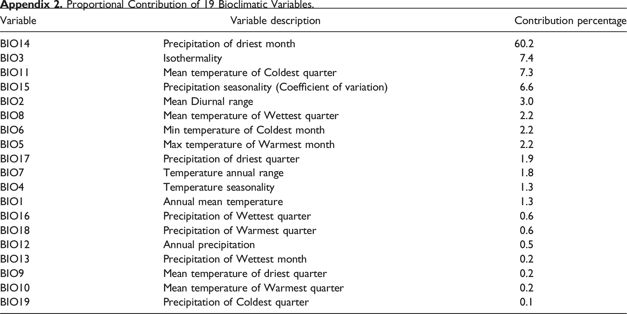
For the margay potential distribution model, 202 unique locations (coordinates) from México, including 21 locations obtained recently for Michoacán state during the 2007-2020 period,were used. The species potential distribution model exhibited adequate performance with an AUC of 0.96 and a “partial-roc” of 1.85 p<0.00. The crucial variables in the model generation were precipitation in the driest month (60.2%), isothermality (7.4%), and precipitation seasonality (6.6%) (Appendix 2).

The model generated for the state indicates suitable climatic conditions for the potential presence of margay in 82% of the state’s area if we consider all vegetation types and land uses. However, primary tropical or temperate forests are considered suitable habitats, constituting 50% of the state area or 13,061 km² of tropical and 15,576 temperate forests (Table 1). Fragmentation of native forests is broad across the state, but 116 forest stands were identified as containing suitable conditions for the margay, including seven (6% of suitable distribution) corresponding to protected areas. Three extend partially over the Biosphere Preserve Zicuiran-Infiernillo (RBZI by its Spanish acronym). Of these three, the one with the largest protected surface has a size of 2,197 km², 935.7 km² including under protection; another has an area of 3,647.7 km², and 7.8 km² under protection, and the last one that overlapped with the RBZI has an area of 6075.8 km², with 13.2 protected. Only one patch overlapped with the Tancitaro Mountain National Park. It has an area of 17,357 km², with 110.4 km² protected. Another forest stand overlaps with the Lagunas Costeras y serranías Patrimonial Reserve. This patch has an area of 83.5 km², with 28.4 km² protected. Another patch, extending over the El Jorullo Volcano Patrimonial Reserve, has an area of 11.3 km², with 7.7 km² protected. The last one extends over the Urban Ecological Park of Uruapan; it has an area of 65.3 km², with0.5 km² protected. Of the 11,597.9 km² we propose as primary habitat for the margay, only 1,103 km² (9.5%) are under protection.

Table 1.

Land Use Area in Distribution Model of Margay in Central Western Forests in Michoacán, México.

Vegetation type	Surface in Michoacán km²	Presence km²	No presence km²	Presence (%)	No presence (%)
Agriculture	15,849	11,678.50	4,170.40	73.69	26.31
Human settlements	858	585.5	272.5	68.24	31.76
Induced grasslands	6,165	5,536.30	629	89.80	10.20
Temperate forests	15,851	15,576.30	274.9	98.26	1.73
Tropical forests	17,442	13,061.70	4,380.40	74.89	25.11
Bodies of water	832.7	563.3	269.4	67.65	32.35
Mangroves	15.4	13.8	1.6	89.61	10.39
Popal-tular	117.7	112	5.7	95.16	4.84
No vegetation	66.3	61.4	4.9	92.61	7.39

In terms of ecoregions, suitable conditions were identified in decreasing area extent as follows: the Jalisco dry forest, the Sierra Madre del Sur pine-oak forests, and the Trans-Mexican volcanic belt pine-oak forests (Figure 2). In terms of forest categories, the potential distribution included 98.2% of the remaining temperate forests and 74.8% of the tropical forests (Table 1).

Figure 2.

Probability of Margay Presence in Michoacán.

The patches averaged 99.9 km² and ranged from 11.3 to 2,414.7 km² (the largest continuous stand of natural vegetation on the estate). The number of fragments and their size differed among forest categories (Table 1). From the 116 suitable patches, 21 were selected as the most important for connectivity according to the IIC analysis (Figure 3). These averaged 434.4 km², differing in size and forest category. In nine stands, the predominant forest category was tropical dry deciduous forest (Mean: 776.9: range = 63.9 km² to 2,414.7 km²), six in pine-oak forest (Mean: 94.2 km²: range = 64.5 km 2 to 206.2 km²), 5 in pine forest (296.3 km 2 average area ranging from 104.7 km² to 602.1 km²), and one in medium deciduous forest (83.5 km²).

Figure 3.

Integral Index of Connectivity.

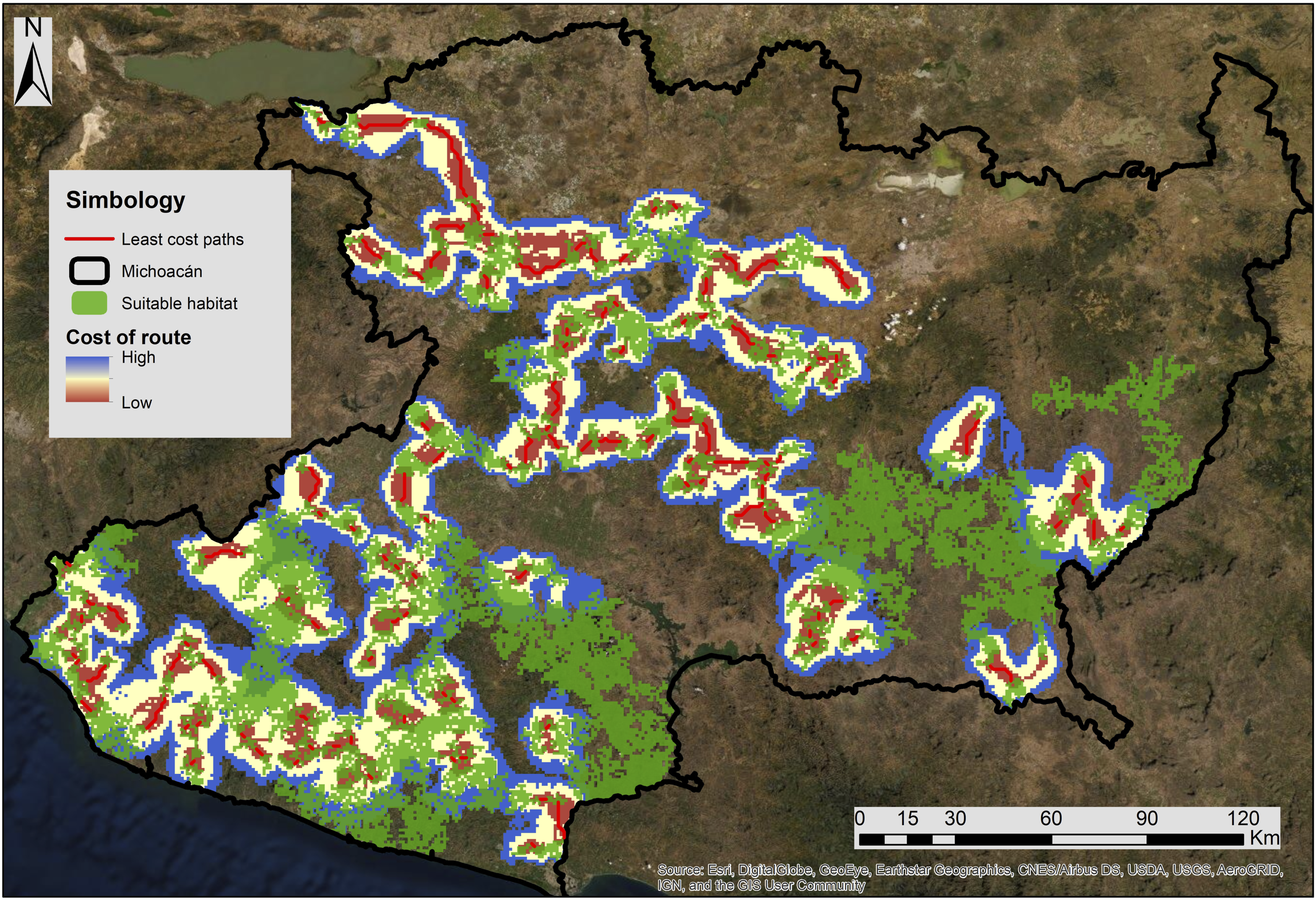
The circuit theory model map indicates how the observed margay areas of activity correlate with suitable habitat and connectivity probability (Figure 4), and the “least-cost paths” model identified 115 potential connectivity routes, which correspond to 476.9 km, averaging 4 km in length, with the longest path measuring 28.2 km (Figure 5). Evaluating the most critical suitable patches, the circuit theory model indicates high connectivity between the Jalisco dry forests and Trans-Mexican volcanic belt pine-oak forests. The lowest connectivity values were observed in the Balsas dry forests. With the “the least cost paths” methodology, 20 paths were designed totaling 598.3 km, with an average of 29.9 km, and the most extended patch measured 989.1 km long. A high overlap existed in the regions between high “probability of connectivity” and “low-cost paths” (Figure 6).

Figure 4.

Probability of Connectivity for Suitable Habitat.

Figure 5.

Least-Cost Paths.

Figure 6.

Probability of Connectivity and Least-Cost Paths for Most Important Patches.

Discussion

The results represent the first assessment in central western México to define suitable primary habitat available and the adequate area for the margay potential use, even though studies implying carnivore connectivity were performed previously (Balbuena-Serrano et al., 2021). Only two studies have assessed feline connectivity in central-western Mexico, including one for bobcats (Correa-Ayram et al., 2014) and another for ocelots (Avila-Coria et al., 2019). Nevertheless, we consider that addressing the habitat and connectivity requirements of the margay is a high priority due to the threat level at which it is listed.

The potential distribution model predicts a high presence probability in the state of Michoacán, and the potential distribution with suitable climatic conditions is significant for the Trans-Mexican volcanic belt pine-oak forests, Jalisco dry forests, and Sierra Madre del Sur pine-oak forests ecoregions, which in addition present also a high proportion of temperate (oak, pine-oak) and tropical forests (semideciduous and deciduous forests) respectively. We recommend paying particular attention to these areas with a high probability of presence for margay because they include areas that could function as habitat for margay. However, these areas face major land use change threats (Mas et al., 2009). Therefore, the presence of the species in these areas could be compromised.

The model exhibits a low presence probability in the Balsas and Bajío dry forests. This result can be explained by the most critical variable in the construction of the model which is the precipitation in the driest month, indicating that in these regions the precipitation levels in the dry season are not enough for margay requirements (Oliveira, 1998). Most relevant variables in model construction differ from those found by other authors (Charre-Medellín, 2009, 2017; Espinosa et al., 2017; Martínez-Calderas et al., 2016). This may result from the difference in the number, dispersion, and localization of records used, the scale at which the model was made, and the variables used to generate the model (Phillips et al., 2006).

Conservation actions should be conducted based on reliable, detailed, and spatially explicit species requirements (Rabinowitz & Zeller, 2010). Our analysis is the first based on specific margin requirements. The margay is probably the most susceptible felid to fragmentation in the state and country along with the jaguar (Oliveira et al., 2015; Quigley et al., 2017; SEMARNAT, 2010), considered vulnerable to human perturbation (Oliveira et al., 2015). Given the current situation in Michoacán regarding the change in land use, where native forests are being lost rapidly while the area of crops is increasing, coupled with the fact that the margay has arboreal habits (Mas et al., 2017), fragmentation of its habitat could threaten its subsistence in the state shortly. Furthermore, the margay needs to hunt to persist as a mesopredator. Margay’s diet includes small mammals such as rodents, birds, reptiles, amphibians, and invertebrates (Bianchi et al., 2011; Cinta-Magallón et al., 2012). Preserving Margay’s habitat involves habitat and prey as well.

Habitat loss and fragmentation affect felids dispersion (Abouelezz et al., 2018; Borah et al., 2016; Elliot et al., 2014), maintaining functional connectivity between isolated habitat patches could maintain gene flow and contribute to metapopulation dynamics (Stockwell et al., 2003). Functional connectivity is a helpful tool in felid conservation since it allows the recognition of areas with functional connectivity that present a greater richness of felids than those without (Gil-Fernandez et al., 2017).

The areas the model indicates as connective must be considered a priority for conservation for decision-makers (McRae et al., 2008). We identified enough habitat patches to maintain multiple margay populations in the state and the potential routes that margays could be used to move between patches. This connectivity would allow the establishment of a connectivity network between the protected natural areas of the central-western region of the country, whose margay populations could be critical in the species adaptability due in this region, the records of felids such as jaguarundi (Herpailurus yagouaroundi), ocelot (Leopardus pardalis), and margay correspond to maximum temperature and driest conditions in which the presence of these felid populations has been recorded in México (Charre-Medellín et al., 2015). Also, Michoacán connects the populations that are the limit of the margay’s distribution to the northern with the central and southern populations in México.

Our study observed high connectivity values in Coahuayana, Aquila, Tumbiscatío, Los Reyes, Uruapan, and Coeneo municipalities. Nevertheless, these regions are considered the main deforestation hotspots in Michoacán due to the advance in avocado cultivation in the Trans-Mexican volcanic belt pine-oak forests ecoregion and the advance of induced grasslands in the Jalisco dry forests and Sierra Madre del Sur pine-oak forests ecoregions (Mas et al., 2009). For this reason, the urgency of applying actions for conservation stands out.

Implications for Conservation

Natural protected areas are essential for conservation, but they alone cannot ensure sufficient habitat protection or effective conservation management for all species. These results provide a diagnosis of the current habitat availability based on margay requirements, highlighting relevant areas for population conservation and vegetation patches that promote connectivity.

Footnotes

Acknowledgments

We want to thank Juan Manuel Ortega Rodríguez^†, Yvonne Herrerías Diego, and José Fernando Villaseñor Gómez for the tips and reviews contributed to the work. We would like to thank the Camorlinga-Torres family for their help in the field. We are also grateful for the field support provided by students from the Laboratory of Priority Terrestrial Vertebrates to the Faculty of Biology for the facilities granted and to the UMSNH for the preparation of the manuscript and Jennifer Siobhan Lowry for assistance in revision.

ORCID iDs

Tiberio C. Monterrubio-Rico

Juan F. Charre-Medellín

Statements and Declarations

Funding

We thank Secretaría de Ciencia, Humanidades, Tecnología e Innovación (SECIHTI)for the master’s scholarship number 704049 and the PhD scholarship number 838168 granted. We also thank the Coordinación para la Investigación Científica at UMSNH for continuous funding of research in endangered species. JFCM thanks SECIHTI for the postdoctoral fellowship awarded.

Conflicting Interests

The authors declared no potential conflicts of interest regarding the research, authorship, and/or publication of this article.

Data Availability Statement

The data supporting this study’s findings are available on request from the corresponding author. *

Appendix

Appendix 1. Values Assigned to the Landscape Variables for the Resistance Matrix.

Land use	Cost value	Vegetation and land use	Cost value	NDVI	Cost value	Human density/Km²	Cost value
Irrigated agriculture	60	Cloud forests/secondary vegetation	10	No natural land uses	100	0 to 1,000	10
Rainfed agriculture	50	Pine-oak forests/primary vegetation	0	−1 to 0	100	1,000 to 2,500	20
Perennial crop	60	Pine-oak forests/secondary vegetation	10	0 to 0.2	80	2,500 to 5,000	30
Human settlements	100	Low tropical deciduous forests/primary vegetation	0	0.2 to 0.4	60	5,000 to 10,000	60
Induced grasslands	50	Low tropical deciduous forests/secondary vegetation	10	0.4 to 0.6	40	10,000 to 20,000	80
Oak forests/primary vegetation	0	Medium tropical deciduous forests/primary vegetation	0	0.6 to 0.8	20	>20,000	100
Oak forests/secondary vegetation	10	Medium tropical deciduous forests/secondary vegetation	10
Oyamel forests/primary vegetation	20	Bodies of water	100
Oyamel forests/secondary vegetation	40	Mangroves	0
Pine forests/primary vegetation	0	Popal-Tular	100
Pine forests/secondary vegetation	10	No apparent vegetation	100
Cloud forests/primary vegetation	0

Appendix 2. Proportional Contribution of 19 Bioclimatic Variables.

Variable	Variable description	Contribution percentage
BIO14	Precipitation of driest month	60.2
BIO3	Isothermality	7.4
BIO11	Mean temperature of Coldest quarter	7.3
BIO15	Precipitation seasonality (Coefficient of variation)	6.6
BIO2	Mean Diurnal range	3.0
BIO8	Mean temperature of Wettest quarter	2.2
BIO6	Min temperature of Coldest month	2.2
BIO5	Max temperature of Warmest month	2.2
BIO17	Precipitation of driest quarter	1.9
BIO7	Temperature annual range	1.8
BIO4	Temperature seasonality	1.3
BIO1	Annual mean temperature	1.3
BIO16	Precipitation of Wettest quarter	0.6
BIO18	Precipitation of Warmest quarter	0.6
BIO12	Annual precipitation	0.5
BIO13	Precipitation of Wettest month	0.2
BIO9	Mean temperature of driest quarter	0.2
BIO10	Mean temperature of Warmest quarter	0.2
BIO19	Precipitation of Coldest quarter	0.1

References

Ávila-Coria

Villavicencio-García

Guerrero-Vázqiez

Treviño-Garza

(2019). Conectividad del paisaje y corredores de hábitat para el ocelote (Leopardus pardalis) y el venado cola blanca (Odocoileus virginianus) en el Occidente de México. Revista de desarrollo urbano y sustentable, 5(17), 38–52. https://doi.org/10.35429/JUSD.2019.17.5.38.52

Ávila-Coria

Villavicencio-García

Muñiz-Castro

M. Á.

Treviño-Garza

(2015). Conectividad del hábitat forestal del ocelote (Leopardus pardalis) en la Sierra de Quila y zonas adyacentes, estado de Jalisco, México. Memorias de resúmenes en extensor SELPER-XXI-México-UACJ-2015 CONECTIVIDAD.

Abouelezz

H. G.

Donovan

T. M.

Mickey

R.M.

Murdoch

J. D.

Freeman

Royar

K. J.

(2018). Landscape composition mediates movement and habitat selection in bobcats (Lynx rufus): implications for conservation planning. Landscape Ecology, 33, 1301–1318. https://doi.org/10.1007/s10980-018-0654-8

Adriaensen

Chardon

De Blust

Swinnen

Villalba

Gulinck

Matthysen

, et al. (2003). The application of ‘least-cost’modelling as a functional landscape model. Landscape and urban planning, 6(4), 233–247.

Alexander

J. L.

Olimb

S. K.

Bly

K. L. S.

Restani

(2016). Use of least-cost path analysis to identify potential movement corridors of swift foxes in Montana. Journal of Mammalogy, 97(3), 891–898. https://doi.org/10.1093/jmammal/gyw032

Almasieh

Kaboli

Beier

(2016). Identifying habitat cores and corridors for the Iranian black bear in Iran. Ursus, 27(1), 18–30. https://doi.org/10.2192/URSUS-D-15-00032.1

Almazán-Catalán

J. A.

Sánchez-Hernández

Ruíz-Gutiérrez

Romero-Almaráz

M. de L.

Taboada-Salgado

Beltrán-Sánchez

Sánchez-Vázquez

(2013). Registros adicionales de felinos del estado de Guerrero, México. Revista Mexicana de Biodiversidad, 84, 347–359. https://doi.org/10.7550/rmb.23087

Aranda

Valenzuela-Galván

(2015). Registro notable de margay (Leopoardus wiedii) en el bosque mesófilo de montaña de Morelos, México. Revista Mexicana de Biodiversidad, 86, 1110–1112. https://doi.org/10.1016/j.rmb.2015.09.015

Araya-Gamboa

Salom-Pérez

(2015). Identificación de sitios de cruce de fauna en la ruta 415, en el “Paso del Jaguar”. Costa Rica. Revista Infraestructura Vial, 17(30), 5–12.

10.

Ashrafzadeh

M.R.

Khosravi

Adibi

M.A.

Taktehrani

Wan

H.Y.

Cushman

S.A.

(2020). A multi-scale, multi-species approach for assessing the effectiveness of habitat and connectivity conservation for endangered felids. Biological Conservation, 245, 108523. https://doi.org/10.1016/j.biocon.2020.108523

11.

Balbuena-Serrano

Á.

Mariela Zarco-González

Carreón-Arroyo

Carrera-Treviño

Amador-Alcalá

Monroy-Vilchis

(2021). Connectivity of priority areas for the conservation of large carnivores in northern Mexico. Journal for Nature Conservation. https://doi.org/10.1016/j.jnc.2021.126116

12.

Beier

Majka

Spencer

(2007). Forks in the road: choices in GIS procedures for designing wildland linkages. Conservation Biology, 1–22. https://doi.org/10.1111/j.1523-1739.2008.00942.x

13.

Bezaury-Creel

J.E.

Torres

J. Fco.

Ochoa-Ochoa

L. M.

Castro-Campos

Moreno

(2009). Base de Datos Geográfica de Áreas Naturales Protegidas Estatales, del Distrito Federal y Municipales de México - Versión 2.0, Julio 31, 2009. The Nature Conservancy / Comisión Nacional para el Conocimiento y Uso de la Biodiversidad / Comisión Nacional de Áreas Naturales Protegidas.

14.

Bianchi

R. de C.

Rosa

A. F.

Gatti

Mendes

S. L.

(2011). Diet of margay, Leopardus wiedii, and jaguarundi, Puma yagouaroundi, (Carnivora: Felidae) in Atlantic Rainforest, Brazil. Zoologia (Curitiba), 28(1), 127–132. https://doi.org/10.1590/S1984-46702011000100018

15.

Borah

Jena

Yumnam

Puia

(2016). Carnivores in corridors: estimating tiger occupancy in Kanha–Pench corridor, Madhya Pradesh, India. Regional Environmental Change, 16, 43–52. https://doi.org/10.1007/s10113-015-0904-0

16.

Botello

Illoldi-Rangel

Linaje

Sánchez-Cordero

(2009). Primer registro de Leopardus wiedii y gato montés en la reserva de la biósfera de Tehuacán-Cuicatlán, Oaxaca, México. Acta Zoológica Mexicana, 22(1), 135–139.

17.

Brodie

J. F.

(2009). Is research effort allocated efficiently for conservation? Felidae as a global case study. Biodiversity Conservation, 18, 2927–2939. https://doi.org/10.1007/s10531-009-9617-3

18.

Carvajal-Villarreal

Caso

Downey

Moreno

Tewes

M. E.

Grassman

L. I.

(2012). Spatial patterns of the margay (Leopardus wiedii; Felidae, Carnivora) at “El Cielo” Biosphere Reserve, Tamaulipas, México. Mammalia, 76(3), 237–244. https://doi.org/10.1515/mammalia-2011-0100

19.

Castilho

C.S.

Hackbart

V.C.

Pivello

V.R.

Santos

R.F.

(2015). Evaluating Landscape Connectivity for Puma concolor and Panthera onca Among Atlantic Forest Protected Areas. Environmental Management, 55, 1377–1389. https://doi.org/10.1007/s00267-015-0463-7

20.

Charre-Medellín

J. F.

(2009). Distribución y diversidad de mamíferos medianos y grandes en el municipio de Arteaga, Michoacán. Universidad Michoacán de San Nicolás de Hidalgo.

21.

Charre-Medellín

J. F.

(2017). Modelado de abundancias potenciales de felinos Silvestres en el trópico seco del centro-occidente de México. Doctoral dissertation. Universidad Michoacán de San Nicolás de Hidalgo. México.

22.

Charre-Medellín

J.F.

Monterrubio-Rico

T.C.

Acevedo

Guzmán-Díaz

E.O.

Jiménez

J.A.

(2021). Jaguar (Panthera onca) density in the Sierra Madre del Sur; the last wilderness area in the central-western slope in Mexico. Studies on Neotropical Fauna and Environment, 58, 47–60. https://doi.org/10.1080/01650521.2021.1895572

23.

Charre-Medellín

J. F.

Monterrubio-Rico

T. C.

Guido-Lemus

Mendoza

(2015). Patrones de distribución de felinos silvestres (Carnivora: Felidae) en el trópico seco del Centro-Occidente de México. Revista de Biología Tropical, 63(3), 783–797. https://doi.org/10.15517/rbt.v63i3.15408

24.

Cinta-Magallón

C. C.

Bonilla-Ruz

C. R.

Alarcón-D

Arroyo-Cabrales

(2012). Dos nuevos registros de margay (Leopardus wiedii) en Oaxaca, México, con datos sobre hábitos alimentarios. Cuadernos de Investigación UNED, 4(1), 33–40. https://doi.org/10.22458/urj.v4i1.131

25.

Comisión Forestal del Estado de Michoacán . (2014). Inventario estatal forestal y de suelos de Michoacán de Ocampo. Morelia, Michoacán.

26.

CONAFOR . (2020). Estimación de la tasa de deforestación en México para el periodo 2001-2018 mediante el método de muestreo. Documento Técnico. México: Comisión Nacional Forestal.

27.

CONANP . (2018). 100 años de conservación en México 1917-2017 Áreas Naturales Protegidas Federales de la República Mexicana. Comisión Nacional de Áreas Naturales Protegidas.

28.

Correa-Ayram

Camilo A.

Mendoza

M. E.

Pérez-Salicrup

D. R.

López-Granados

(2014). Identifying potential conservation areas in the Cuitzeo Lake basin, Mexico by multitemporal analysis of landscape connectivity. Journal for Nature Conservation, 22(5), 424–435. https://doi.org/10.1016/j.jnc.2014.03.010

29.

Crawshaw

P. G.

(1995). Comparative ecology of ocelot (Felis pardalis) and jaguar (Panthera onca) in a protected subtropical. University of Florida.

30.

Cuéllar

Maffei

Arispe

R.L.

Noss

A.J.

(2006). Geoffroy's cats at the northern limit of their range: activity patterns and density estimates from camera trapping in Bolivian dry forests. Studies on Neotropical Fauna and Environment, 41, 169–177. https://doi.org/10.1080/01650520600840001

31.

Decout

Manel

Miaud

Luque

(2012). Integrative approach for landscape-based graph connectivity analysis: A case study with the common frog (Rana temporaria) in human-dominated landscapes. Landscape ecology, 27(2), 267–279. https://doi.org/10.1007/s10980-011-9694-z

32.

de la Torre

J. A.

Núñez

J. M.

Medellín

R. A.

(2017). Habitat availability and connectivity for jaguars (Panthera onca) in the Southern Mayan Forest: Conservation priorities for a fragmented landscape. Biological Conservation, 206, 270–282. https://doi.org/10.1016/j.biocon.2016.11.034

33.

Diario Oficial de la Federación . (2014). Reglamento de la Ley General del Equilibrio Ecológico y la Protección al Ambiente en Materia. Última Reforma Publicada DOF 31-10-2014, 15.

34.

Dickson

B.G.

Roemer

G.W.

Mcrae

B.H.

Rundall

J.M.

(2013). Models of Regional Habitat Quality and Connectivity for Pumas (Puma concolor) in the Southwestern United States. PLoS ONE, 8. https://doi.org/10.1371/journal.pone.0081898

35.

Dueñas-López

Rosas Rosas

O. C.

Chapa-Vargas

Bender

L. C.

Tarango-Arámbula

L. A.

Martínez-Montoya

J. F.

Alcántara-Carbajal

J. L.

(2015). Connectivity among jaguar populations in the Sierra Madre Oriental, México. Therya, 6(2), 449–468. https://doi.org/10.12933/therya-15-257

36.

Elith

Graham

C. H.

Anderson

R. P.

Ferrier

Hijmans

Leathwick

J. R.

Loiselle

B. A.

Moritz

Nakazawa

Y. J.

Overton

J. M. M.

Peterson

A. T.

Philips

S. J.

Scachetti-Pereira

Williams

S. E.

Zimmermann

N. E.

Dudik

Guisan

Wisz

M. S.

(2006). Novel methods improve prediction of species’ distributions from occurrence data. Ecography, 29, 129–151. https://doi.org/10.1111/j.2006.0906-7590.04596.x

37.

Elliot

N.B.

Cushman

S.A.

Macdonald

D.W.

Loveridge

A.J.

(2014). The devil is in the dispersers: predictions of landscape connectivity change with demography. Journal of Applied Ecology, 51, 1169–1178. https://doi.org/10.1111/1365-2664.12282

38.

Escalante

Rodríguez-Tapia

Linaje

Illoldi-Rangel

González-López

(2013). Identification of areas of endemism from species distribution models: Threshold selection and Nearctic mammals. Revista especializada en Ciencias Químico-Biológicas, 16(1), 5–17. https://doi.org/10.1016/S1405-888X(13)72073-4

39.

Espinosa

C. C.

Trigo

T. C.

Tirelli

F. P.

Da Silva

L. G.

Eizirik

Queirolo

Mazim

F. D.

Peters

F. B.

Favarini

O. F.

de Freitas

R. O.

(2017). Geographic distribution modeling of the margay (Leopardus wiedii) and jaguarundi (Puma yagouaroundi): A comparative assessment. Journal of Mammalogy, 20(10), 1–11. https://doi.org/10.1093/jmammal/gyx152

40.

Feng

Park

D. S.

Liang

Pandey

Papes

(2019). Collinearity in ecological niche modeling: Confusions and challenges. Ecology and Evolution, 9(18), 10365–10376. https://doi.org/10.1002/ece3.5555

41.

Gilbert-Norton

Wilson

Stevens

J. R.

Beard

K. H.

(2010). A meta-analytic review of corridor effectiveness. Conservation Biology, 24(3), 660–668. https://doi.org/10.1111/j.1523-1739.2010.01450.x

42.

Gil-Fernández

Muench

Gómez-Hoyos

D. A.

Dueñas

Escobar-Lasso

Aguilar-Raya

Mendoza

(2017). Wild felid species richness affected by a corridor in the Lacandona forest, Mexico. Animal Biodiversity and Conservation, 40(1), 115–123. https://doi.org/10.32800/abc.2017.40.0115

43.

González-Saucedo

Z. Y.

(2011). Conectividad funcional para el puma (Puma concolor) en el centro de México. Master thesis. Universidad Autónoma de Querétaro.

44.

Greenspan

Montgomery

Stokes

Wantai

Moo

S.S.

(2021). Large felid habitat connectivity in the transboundary Dawna-Tanintharyi landscape of Myanmar and Thailand. Landscape Ecology, 36, 3187–3205. https://doi.org/10.1007/s10980-021-01316-5

45.

Hijmans

R. J.

Cameron

S. E.

Parra

J. S.

Jones

P. G.

Jarvis

, (2005). Very high-resolution interpolated climate surfaces for global land areas. Int. J. Climatol, 25, 1965–1978. https://doi.org/10.1002/joc.1276

46.

Hirzel

A. H.

Le Lay

(2008). Habitat suitability modelling and niche theory. Journal of Applied Ecology, 45(5). https://doi.org/10.1111/j.1365-2664.2008.01524.x

47.

Imbernon

Villacorta Monzón

J. L.

Zelaya Flores

C. L.

Valle Aguirre

A. A.

(2005). Fragmentación y conectividad del bosque en El Salvador: Aplicación al Corredor Biológico Mesoamericano. Bois Et Forêts Des Tropiques, 286(4), 15–28.

48.

INEGI . (2014). Conociendo Michoacán de Ocampo. https://www.inegi.org.mxatencion.usuarios@inegi.org.mx.

49.

Kasper

C. B.

Schneider

Oliveira

T. G.

(2016). Home range and density of three sympatric felids in the Southern Atlantic Forest, Brazil. Brazilian Journal of Biology, 76(1), 228–232. https://doi.org/10.1590/1519-6984.19414

50.

Konecny

(1989). Movement Patterns and Food Habits of Four Sympatric Carnivore Species in Belize, Central America. Advances in Neotropical Mammalogy, 243–264.

51.

Liu

White

Newell

(2013). Selecting thresholds for the prediction of species occurrence with presence-only data. Journal of Biogeography, 40(4), 778–789. https://doi.org/10.1111/jbi.12058

52.

Martínez-Calderas

J. M.

Hernández-Saintmartín

A. D.

Rosas-Rosas

O. C.

Palacio-Núñez

Villordo-Galván

J. A.

Olivera-Méndez

(2016). Potential distribution of margay (Leopardus wiedii, Schinz, 1821) in Northeastern Mexico. Therya, 7(2), 241–255. https://doi.org/10.12933/therya-16-360

53.

Mas

Lemoine-Rodríguez

González-López

Piña-Garduño

Herrera-Flores

(2017). Land use / land cover change detection combining automatic processing and visual interpretation. European Journal of Remote Sensing, 50(1), 626–635. https://doi.org/10.1080/22797254.2017.1387505

54.

Mas

J.-F.

Velázquez

Couturier

(2009). La evaluación de los cambios de cobertura / uso del suelo en la República Mexicana. Investigación Ambiental, 1(1), 23–39.

55.

McRae

B. H.

Dickson

B. G.

Keit

T. H.

Shah

V. B.

(2008). Using circuit theory to model connectivity in ecology, evolution and conservation. Ecology, 89(10), 2712–2724. https://doi.org/10.1890/07-1861.1

56.

Monroy-Vilchis

Zarco-González

M. M.

(2019). Potential distribution and areas for conservation of four wild felid species in Mexico: conservation planning. Mammalian Biology. https://doi.org/10.1016/j.mambio.2019.09.003

57.

Monterrubio-Rico

T.C.

Charre-Medellín

J.F.

Pérez-Martínez

M.Z.

Mendoza

(2017). Use of remote cameras to evaluate ocelot (Leopardus pardalis) population parameters in seasonal tropical dry forests of central-western Mexico. Mammalia, 82, 113–123. https://doi.org/10.1515/mammalia-2016-0114

58.

Monterrubio-Rico

T.C.

Medellín

J.F.

Páramo

M.G.

Camacho

H.C.

Rivera

M.Q.

Paniagua

L.L.

(2012). Evidencias fotográfica, biológica y genética de la presencia actual de jaguaroundi (Puma yagouaroundi) en Michoacán, México. Revista Mexicana De Biodiversidad, 83, 825–833. https://doi.org/10.7550/rmb.28663

59.

Moratelli

de Andreazzi

C. S.

de Oliveira

J. A.

Cordeiro

J. L. P.

(2011). Current and potential distribution of Myotis simus (Chiroptera, Vespertilionidae). Mammalia, 75, 227–234. https://doi.org/10.1515/mamm.2011.028

60.

Muhammed

Anandhi

Chen

(2022). Comparing Methods for Estimating Habitat Suitability. Land, 11(10). https://doi.org/10.3390/land11101754

61.

Nagy-Reis

Oshima

J. E. D. F.

Kanda

C. Z.

Palmeira

F. B. L.

de Melo

F. R.

Morato

R. G.

de Almeida

L. B.

Magioli

Rohi

Martello

da Silva

R. A.

dos Santos

J. A.

Priante

Rogeri

Gaspar

Canteri

Trinca

C. T.

Pagila

A. P.

Gatica

Ribeiro

M. C.

(2020). Neotropical Carnivores: a data set on carnivore distribution in the Neotropics. Ecology, 101.

62.

Oliveira

T. G.

(1998). Mammalian Species, Leopardus wiedii. American Society of Mammologists, (579), 1–6.

63.

Oliveira

T. G.

Paviolo

Schipper

Bianchi

Payan

Carvajal

S.V.

(2015). Leopardus wiedii. The IUCN Red List of Threatened Species.

64.

Oliveira

T. G. D

Tortato

M. A

Silveira

Kasper

C. B.

Mazim

F. D.

Lucherini

Jácomo

A. T. A.

Soares

J. B. G.

Marques

R. V.

Sunquist

(2010). Ocelot ecology and its effect on the small-felid guild in the lowland neotropics. In MacDonald

D. W.

Loveridge

A. J.

(Eds.), Biology and conservation of wild felids (pp. 559–580): OXFORD University Press.

65.

Osorio-Olvera

L. A.

Falconi

Soberon

(2016). On the relationship between habitat suitability and population abundance under different dispersal scenarios. Rev. Mex. Biodivers, 87, 1080–1088. https://doi.org/10.1016/j.rmb.2016.07.001

66.

Pascual-Hortal

Saura

(2006). Comparison and development of new graph-based landscape connectivity indices: towards the prioritization of habitat patches and corridors for conservation. Landscape ecology, 21, 959–967. https://doi.org/10.1007/s10980-006-0013-z

67.

Pérez-Irineo

Santos-Moreno

(2016). Abundance and activity patterns of medium-sized felids (Felidae, Carnivora) In Southeastern Mexico. The Southwestern Naturalist, 61(1), 33–39. https://doi.org/10.1894/0038-4909-61.1.33

68.

Pérez-Irineo

Santos-Moreno

Hernández-Sánchez

(2017). Density and activity pattern of Leopardus wiedii and Leopardus pardalis in Sierra Norte of Oaxaca, Mexico. Therya, 8(3), 223–232. https://doi.org/10.12933/therya-17-487

69.

Peterson

A. T.

Papes

Soberón

(2008). Rethinking receiver operating characteristic analysis applications in ecological niche modeling. Ecological modeling, 2012 (2008), 63-72. https://doi.org/10.1016/j.ecolmodel.2007.11.008

70.

Phillips

S. J.

Anderson

R. P.

Schapire

R. E.

(2006). Maximum modeling entropy of species geographic distributions. Ecological Modelling, 190, 231–239. https://doi.org/10.1016/j.ecolmodel.2005.03.026

71.

Qiao

Soberón

Peterson

A.T.

(2015). No silver bullets in correlative ecological niche modelling: insights from testing among many potential algorithms for niche estimation. Methods in Ecology and Evolution, 6. https://doi.org/10.1111/2041-210X.12397

72.

Quigley

Foster

Petracca

Payan

Salom

Harmsen

(2017). Panthera onca (errata version published in 2018). The IUCN Red List of Threatened Species.

73.

Rabinowitz

A.R.

Zeller

K.A.

(2010). A range-wide model of landscape connectivity and conservation for the jaguar, Panthera onca. Biological Conservation, 143, 939–945. https://doi.org/10.1016/j.biocon.2010.01.002

74.

Resasco

(2019). Meta-analysis on a decade of testing corridor efficacy: What new have we learned? Current Landscape. Ecology Reports, 4, 61–69. https://doi.org/10.1007/s40823-019-00041-9

75.

Rodríguez-Soto

Monroy-Vilchis

Zarco-González

M. M.

(2013). Corridors for jaguar (Panthera onca) in Mexico: Conservation strategies. Journal for Nature Conservation, 21(6), 438–443. https://doi.org/10.1016/j.jnc.2013.07.002

76.

Salazar

Mendoza

Ochoa-Gaona

Ku-Quej

Hidalgo-Mihart

(2017). Evaluación de la conectividad del paisaje en la región Puuc-Chenes, México, con base en los requerimientos de hábitat del jaguar (Panthera onca). Investigaciones Geográficas, 2017(92), 101–115. https://doi.org/10.14350/rig.52210

77.

Saura

Torné

(2009). Conefor Sensinode 2.2: a software package for quantifying the importance of habitat patches for landscape connectivity. Environmental Modelling & Software, 24, 135–139. https://doi.org/10.1016/j.envsoft.2008.05.005

78.

SEMARNAT . (2010). Norma Oficial Mexicana NOM-059-SEMARNAT-2010. Diario Oficial de la federación.

79.

Soberón

Osorio-Olvera

Peterson

(2017). Diferencias conceptuales entre modelación de nichos y modelación de áreas de distribución. Revista Mexica de Biodiversidad, 88 (2017), 437-444. https://doi.org/10.1016/j.rmb.2017.03.011

80.

Stockwell

C.A.

Hendry

H.P.

Kinnison

M.T.

(2003). Contemporary evolution meets conservation biology. Trends in Ecology and Evolution, 18, 94–101. https://doi.org/10.1016/S0169-5347(02)00044-7

81.

Sunquist

(2002). Wild Cats of the World. The University of Chicago Press, Chicago and London.

82.

Tischendorf

Fahrig

(2000). On the usage and measurement of landscape connectivity. Oikos, 90(1), 7–19.

83.

Tobler

M.W.

Powell

G.V.

(2013). Estimating jaguar densities with camera traps: Problems with current designs and recommendations for future studies. Biological Conservation, 159, 109–118. https://doi.org/10.1016/j.biocon.2012.12.009

84.

Van den Berg

C. M.

(2021). Analyzing landscape connectivity for Felidae in Oaxaca given current and potential community land use trends. Master thesis. Duke University.

85.

Wallace

R. B.

Gómez

Porcel

Z. R.

Rumiz

(2010). Distribución, Ecología y Conservación de los mamíferos medianos y grandes de Bolivia (pp. 55–73): Centro de.

86.

Wang

Feng

Zhang

Fan

Tang

Dong

Zhang

Zhou

Bai

(2022). Assessment of habitat suitability and connectivity across the potential distribution landscape of the sambar (Rusa unicolor) in Southwest China. Frontiers in Conservation Science, 3. https://doi.org/10.3389/fcosc.2022.909072

87.

Wei

Wang

Hou

Wang

(2018). Predicting the current and future cultivation regions of Carthamus tinctorius L. using Maxent model under climate change in China. Global Ecology and Conservation, 16, 1–12. https://doi.org/10.1016/j.gecco.2018.e00477

88.

Wikramanayake

E.D.

McKnight

M.W.

Dinerstein

Joshi

A.R.

Gurung

Smith

D.E.

(2004). Designing a Conservation Landscape for Tigers in Human-Dominated Environments. Conservation Biology, 18. https://doi.org/10.1111/j.1523-1739.2004.00145.x

89.

Zeller

K. A.

Mcgarigal

Whiteley

A. R.

(2012). Estimating landscape resistance to movement: a review. Landscape Ecology, 27, 777–797. https://doi.org/10.1007/s10980-012-9737-0

Assessing Suitable Habitat and Functional Connectivity for Margay ( Leopardus wiedii ) in Central Western Forests in Michoacán,México

Abstract

Keywords

Introduction

Methods

Results

Discussion

Implications for Conservation

Footnotes

Acknowledgments

ORCID iDs

Statements and Declarations

Funding

Conflicting Interests

Data Availability Statement

Appendix

References