Sage Journals: Discover world-class research

Abstract

Background:

The adoption of continuous glucose monitoring (CGM) already helps to improve glycemic control in diabetes. When coupled with appropriate data analysis techniques, CGM also provides dependable estimates for significant metrics, like glycated hemoglobin (HbA1c). Findings from the REALISM-T1D study can boost HbA1c estimation methods in diabetes care and stimulate their use in clinical practice.

Methods:

Continuous glucose monitoring data of 27 adults affected by type-1 diabetes were acquired by means of G6 (Dexcom, San Diego, CA) sensors for a time span of 120 days. Glycated hemoglobin laboratory assays were performed during the concluding follow-up visits. Data were then analyzed to derive estimates of assay results, taken as the gold standard.

Results:

Bland-Altman (BA) plots show that smart interpolation to patch missing data and a wise choice of interstitial glucose (IG) weighting function, besides a proper mean interstitial glucose (MIG) to HbA1c regression equation, improve HbA1c estimation quality with respect to methods relying on MIG alone. A decrease in the BA plot-related variance of differences with respect to the gold standard confirms the improvement. Wilcoxon signed-rank tests on the bias-compensated mean squared error (MSE) with respect to conventional MIG-based methods show that the improvement is statistically significant with a confidence level better than 95% (P = .0179).

Conclusions:

Improved HbA1c estimation methods result in better HbA1c prediction quality with respect to those based on MIG alone, thus providing quick, but still relatively accurate feedback to diabetologists. They alleviate the discordances reported in literature and, with further improvements, may become a viable complement/alternative to HbA1c assays.

Keywords

continuous glucose monitoring glycated hemoglobin estimation prediction models real-life observation type-1 diabetes

Background

Glycated hemoglobin (HbA1c) assays are common practice to judge long-term glycemic control in diabetes care, and calibration techniques have been internationally standardized and refined over the years to assess the precision and accuracy of commercial HbA1c measurement methods.^1,2 Real-time continuous glucose monitoring (RT-CGM), in turn, allows to collect lots of glucose data,³ which can be used to estimate HbA1c without resorting to laboratory tests.⁴

The evaluation of estimated HbA1c from CGM, also known as eA1C or glucose management indicator (GMI),⁵ and its relationships with average glucose values were investigated in a number of studies.^4,6-8 A good agreement between eA1C/GMI and the reference gold standard HbA1c can significantly help clinicians in achieving better disease monitoring and control and healthcare managers in lowering overall healthcare costs. However, as discrepancies exist between predicted and assay values of HbA1c,^9,10 improvements in the mathematical methods can reduce differences and allow users to gain more confidence in the estimations themselves.

Moreover, CGM introduces other sources of uncertainty when carried out in real-life situations¹¹ because the collection of glucose values performed at home is frequently subject to device misuse and wrong patient behavior, thus resulting in missing and/or incorrect sensor data¹² that may affect estimation quality. The “REAl-Life glucoSe Monitoring in Type 1 Diabetes” (REALISM-T1D) observational study is aimed at evaluating the advantages that can be obtained by adopting CGM in real-life conditions for adult patients affected by type-1 diabetes. We have focused on the improvement of CGM-based estimation methods, with the aim of obtaining better predicted values for HbA1c.

A popular eA1C estimation method proposed by Leow¹³ is based on 3 steps (Figure 1). First the area under curve (AUC) is evaluated by integration of the curve of interstitial glucose (IG) sensor values over time. Then AUC is used to compute the mean interstitial glucose (MIG) value and finally a mapping function (the regression equation from the ADAG study⁴ or other equations^6,14-16) derives eA1C from MIG. Leow’s method¹³ did not focus on the collection, filtering, and management of missing sensor data. Moreover, AUC was computed without using any weighting function w(t) for CGM samples, though this possibility was mentioned in Leow’s paper.

Figure 1.

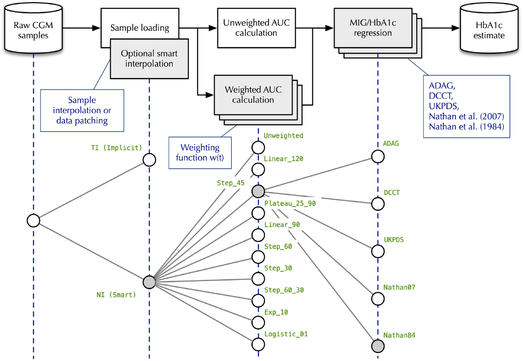
General procedure of HbA1c estimation from CGM samples and test plan. CGM, continuous glucose monitoring.

This paper explores the degrees of freedom in the eA1C evaluation method to reduce its discrepancies with respect to the HbA1c assays. To this purpose, we considered the combined effects of 3 factors:

Management of missing sensor data collected in real-life conditions through commercial devices and software.

Adoption of a weighting function in the integration of the IG curve to evaluate MIG.

Use of different MIG to eA1C regression equations widely adopted in the literature studies.

Methods

A total of 33 Caucasian patients in north-western Italy were invited to take part in the study. Four of them declined the invitation while the others signed a voluntary informed consensus to participate. To grant personal data protection, pseudonymization was adopted and transcoding tables were stored in protected servers of the care center.

Inclusion criteria were age between 18 and 70 years, type-1 diabetes, stable complications, and acquired habit to wear CGM devices for 6 months or more. No constraints were imposed on the metabolic compensation in terms of HbA1c at the baseline. Exclusion criteria were the presence of severe complications at an advanced stage, uncompensated psychiatric disorders, and possibly dangerous societal problems. As the study was designed as purely observational, there was no need for a control group monitored with blinded devices. Other study requirements were the adoption of CGM in real-life conditions, continuous data recording for 120 days at least, and the use of the CGM sensor for at least 65% of the time during the whole observation period.

The initial group size was determined based on the requirements for the statistical significance of the Wilcoxon signed-rank test, planned for use to compare HbA1c estimation methods. Calculations were performed according to Divine et al¹⁷ based on ɑ =.10 (probability of type-I error) and β = .20 (probability of type-II error).

Moreover, it was conservatively assumed that, in the notation of Divine et al., Pʹ = .8. This corresponds to an 80% probability that, for a given pair of HbA1c estimations pertaining to the same patient and derived by different methods, the difference between their bias-compensated squared errors is greater than zero. No compensation for ties was applied because they were not expected to occur. The assessment gave a minimum required sample size of N = 23, then increased to 33 to account for dropouts and uncertainties in the estimation of Pʹ.

At the baseline, the group consisted of 29 people (14 male and 15 female), had a mean age of 43.8 ± 14.8 years (mean ± standard deviation, range 18–69), disease duration of 24.9 ± 13.5 years (range 3–56), body mass index (BMI) of 24.2 ± 3.3 kg/m² (range 20-31), and HbA1c of 7.1% ± 1.0% or 54 ± 10 mmol/mol (range 5%-9% or 31-75 mmol/mol). At the end of the observation period 2 patients did not satisfy the 65% sensor use requirement and were not included in the subsequent statistical analysis.

Patients were instructed about the use of prescribed commercial G6 (Dexcom, San Diego, CA) devices, which were fully reimbursable and repaid by the Italian National Health System, and procedures to upload CGM data to the DIASEND (Glooko, Mountain View, CA) and CLARITY (Dexcom, San Diego, CA) websites. Since the study was purely observational, participation did not affect the behavior and decision of the care team, and patients were let free to manage the everyday use of their devices.

Data collection was carried out between January 1 and May 31, 2021. A follow-up visit was planned at the end of the period, when an HbA1c laboratory assay was performed based on high-performance liquid chromatography (HPLC) ion-exchange chromatography.¹⁸

The upper part of Figure 1 summarizes how eA1C can be derived from CGM measurements according to Leow.¹³ Gray rectangles in the figure represent data processing blocks, and arrows specify data flow. The lower part of the figure summarizes the choices that can be made in each processing block.

CGM data are acquired from the CGM vendor’s or third party’s web-based portal and preprocessed. Two different ways of dealing with missing samples were explored:

Leave this duty to the next processing block, area under curve (AUC) calculation, which is capable of handling nonuniformly spaced data. This approach, called TI, is mathematically straightforward but cannot consider the contributions of missing data samples resulting from the action of biochemistry mechanisms for blood glucose regulation.

Synthesize missing samples with a patching strategy, aware of the kind of information it is working on. The strategy explored in this work, called NI, is still based on interpolation when the amount of missing data is less than 4 hr, using a technique similar to the one described by Fonda et al.¹² Instead, when the amount of missing data is more than 4 hr, but less than 7 days, it replicates an analogous slice taken from other CGM data stream sections. Although sophisticated techniques have been proposed to deal with missing experimental data,¹⁹ in this study, we are mainly interested in showing that the estimation of HbA1c can be improved in a number of ways with respect to conventional methods currently in use, and even the introduction of elementary signal patching methods can bring tangible benefits. In fact, basic approaches such as those adopted in this paper can reach this goal without resorting to complex and computation-intensive software solutions. Then, short sequences of missing data (eg, intervals shorter than 4 hr corresponding to 48 CGM samples) were dealt with effectively by means of linear interpolation techniques.¹² Moreover, we decided to manage possible larger gaps corresponding to some days of missing CGM data (up to 7 days in our observations) by assuming, for each patient, small changes in the daily mean IG. We are conscious that this assumption can be unrealistic in a number of situations, but we found that cumulative effects of relatively fast variations in the CGM signal on the eA1C computation over a long time period (120 days) were limited in case of satisfactory CGM sensor use. Thus, in this case, imputation of missing elements was performed with the mean IG value computed from the available samples of a time-shifted interval of equal length. Owing to the regular time-spacing of CGM data and the analysis algorithms, this is equivalent to substitute the unavailable pattern with samples in the corresponding shifted interval. The main advantage of this choice is the ability to carry out simpler and faster computations in determining eA1C.

The output of the first step is a stream of IG samples. The next step is AUC calculation, which can in turn be performed in 2 ways:

An unweighted numerical integration of the IG samples based on trapezoidal integration and compatible with Leow’s approach.¹³ To avoid interpolation issues when data are missing at the extreme left of the integration interval, a single artificial sample with the same value as the nearest real sample has been added if needed. This method calculates AUC as: $A U C = \int_{t 1}^{t 2} i g (t) d t$ , where $i g (t)$ represents the IG value sampled at time $t$ and $[t_{1}, t_{2}]$ is the observation interval; the width $d = t_{2} - t_{1}$ of the observation interval has been set to $d = 120 days$ . From AUC, the mean IG across the observation interval can then be calculated by dividing AUC by $d$ : $M I G = A U C / d = 1 / d \int_{t 1}^{t 2} i g (t) d t$ . Given the relatively large number of samples in a typical integration interval (about 34,000 in a 120-day integration interval with 5-min sample spacing) neither the integration method nor boundary effects are likely to introduce any significant difference.

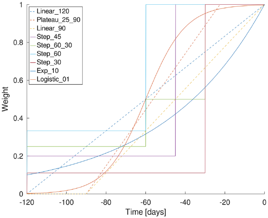
Since several studies^20-22 indicate that the relative importance of IG samples in determining the HbA1c estimation decreases as their temporal distance from the HbA1c sampling point increases, it may be convenient to introduce an IG weighting function w(t) in AUC calculation. In this case, MIG is calculated as $M I G = 1 / W \int_{t 1}^{t 2} w (t - t 2) i g (t)$ . The normalization factor must be $W = \int_{- d}^{0} w (t) d t$ , so that a constant w(t) yields the same result as the previous approach. Figure 2 depicts the 9 w(t) considered in this paper and their names. The steepness of the exponential decay function Exp_10 has been chosen so that $w (- d) = 1 / 10 w (0)$ . The midpoint of the logistic sigmoid Logistic_01 has been set to $- d / 2$ , and its growth rate to 0.1. To justify the empirical selection of these $w (t)$ , it is worth remarking that the purpose of considering weight functions in this study was to assess whether they could improve HbA1c estimation, rather than finding an optimal w(t).

Figure 2.

IG weighting functions w(t) adopted in the study for AUC calculation. IG, interstitial glucose; AUC, area under curve.

The final step in HbA1c estimation involves the use of one of the MIG/HbA1c linear regression equations published in literature and listed in the Appendix, namely, those proposed in the ADAG study,⁴ the UKPDS trial,¹⁴ the DCCT study,¹⁵ and 2 others presented by Nathan et al.^6,16 They are referred to as ADAG, UKPDS, DCCT, Nathan07, and Nathan84, respectively.

The combination of 2 different interpolation techniques, 10 weighting functions (including a constant w(t) for unweighted AUC calculation), and 5 regression equations led to a total of 100 points in the experiment space. This space was explored to find the method that provided the best eA1C. The comparison was performed by means of Bland-Altman (BA) plots,²³ using the variance of the differences with respect to the HbA1c gold standard as a metric.

At first, the exploration was carried out in 2 sequential steps to reduce the number of test cases. In the first step, estimation methods were compared with respect to the data interpolation technique and the w(t) shown in Figure 2, using the ADAG linear regression as in Leow.¹³ The second step started from the most promising interpolation technique and w(t) identified in the first, varying the MIG/HbA1c linear regression equation. Since the 2 analysis steps may be mutually dependent, an exhaustive experiment space exploration was later performed, confirming that the best method identified in this way was still the same as before.

Results

Table 1 lists the main BA plot statistics calculated during the incremental analysis. From left to right, its columns contain:

The name of the test case, given by the concatenation of the interpolation method (NI or TI), the w(t) (one of the names in Figure 2), and the linear regression function (Unweighted, ADAG, DCCT, UKPDS, Nathan07, or Nathan84).

The Spearman’s Rank Correlation Coefficient of the eA1c with respect to the gold standard.

The P value of the mean/difference Spearman’s Rank Correlation R being non-zero, according to a Student’s t-test on the statistic $t = R \sqrt{N - 2} / \sqrt{1 - R^{2}}$ . A P value below a certain threshold $α$ , typically $α = 0.05$ , would suggest that a regression model would be more appropriate than a BA plot for analysis.

The mean squared error (MSE) of eA1C with respect to the gold standard.

The bias and variance of the differences of the test case with respect to the gold standard.

Table 1.

Bland-Altman Plot Statistics for the Experiment Space Considered in the Study.

Test case	Correlation	P	MSE	Bias	Variance
First step, interpolation and w(t) selection
TI_Unweighted_ADAG	0.9081	.1838	0.3453	0.3865	0.2035
TI_Linear_120_ADAG	0.9194	.2011	0.3190	0.3609	0.1960
TI_Plateau_25_90_ADAG	0.9127	.1934	0.3032	0.3401	0.1947
TI_Linear_90_ADAG	0.9139	.2184	0.3004	0.3354	0.1952
TI_Step_45_ADAG	0.9164	.3366	0.2531	0.3047	0.1664
TI_Step_60_30_ADAG	0.9127	.2520	0.2992	0.3532	0.1811
TI_Step_60_ADAG	0.9096	.1923	0.3124	0.3579	0.1914
TI_Step_30_ADAG	0.9096	.5583	0.2858	0.3365	0.1792
TI_Exp_10_ADAG	0.9188	.2208	0.3071	0.3505	0.1913
TI_Logistic_01_ADAG	0.9194	.1817	0.2993	0.3375	0.1926
NI_Unweighted_ADAG	0.9277	.2507	0.2985	0.3741	0.1646
NI_Linear_120_ADAG	0.9435	.3151	0.2675	0.3438	0.1550
NI_Plateau_25_90_ADAG	0.9368	.3288	0.2570	0.3297	0.1540
NI_Linear_90_ADAG	0.9368	.2945	0.2547	0.3249	0.1549
NI_Step_45_ADAG	0.9429	.3589	0.2379	0.3126	0.1455
NI_Step_60_30_ADAG	0.9332	.3181	0.2674	0.3439	0.1549
NI_Step_60_ADAG	0.9432	.2507	0.2685	0.3472	0.1536
NI_Step_30_ADAG	0.9228	.4829	0.2725	0.3294	0.1703
NI_Exp_10_ADAG	0.9447	.3460	0.2609	0.3359	0.1538
NI_Logistic_01_ADAG	0.9368	.2974	0.2543	0.3292	0.1516
Second step, regression equation selection
NI_Step_45_DCCT	0.9429	.1745	0.1881	-0.2545	0.1280
NI_Step_45_UKPDS	0.9429	.1745	0.2144	0.3006	0.1288
NI_Step_45_Nathan07	0.9429	.8894	0.2491	0.3529	0.1293
NI_Step_45_Nathan84	0.9429	.7188	0.3482	0.4760	0.1263

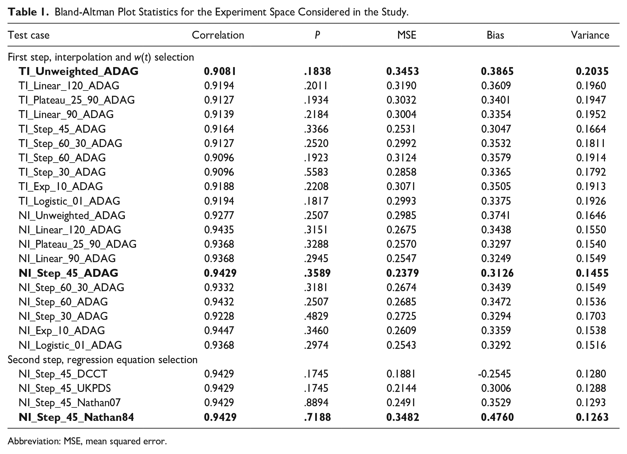
Abbreviation: MSE, mean squared error.

Rows highlighted in bold represent the baseline technique presented in Leow¹³ (implicit interpolation, unweighted AUC calculation, and ADAG regression equation), the best method according to the BA variance of the differences after the first analysis step (smart interpolation, Step_45 w(t), and ADAG regression equation) and after the second (smart interpolation, Step_45 w(t), Nathan84 regression equation). We observe that:

There is little change in the Spearman’s Rank Correlation Coefficient across all test cases, thus confirming that, as also shown in other works,²⁴ this metric is inconclusive to show evidence of any improvement among the methods being analyzed.

The P values of the mean/difference Spearman’s Rank Correlation being non-zero are all above 0.17, thus confirming that BA plots are indeed a well-founded analysis tool in this case.

Discussion

Changing the interpolation technique, w(t) and regression equation does influence HbA1c estimation quality. The NI_Step_45_Nathan84 technique reduces the variance of the differences with respect to the gold standard from 0.2035 to 0.1263 when compared to the baseline technique TI_Unweighted_ADAG,¹³ an improvement of about 38%.

The upper part of Figure 3 contrasts their BA plots (TI_Unweighted_ADAG on the left and NI_Step_45_Nathan84 on the right). In the plots, the dashed horizontal line is the zero-difference line. The middle solid horizontal line marks the mean difference (Bias column of Table 1). The 2 other horizontal lines represent the estimated limits of agreement. They delimit the region around the mean difference within ±1.96 standard deviation of the differences, where 95% of differences between measurements by the 2 methods are expected to lie.

Figure 3.

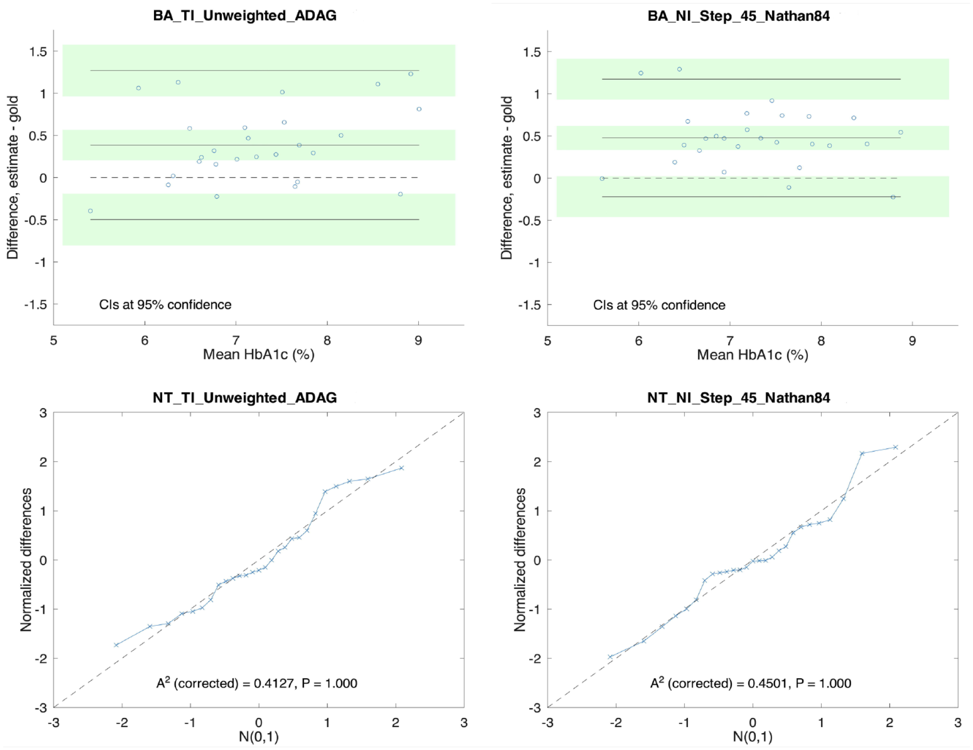
Bland-Altman (BA) plots, quartile-quartile (QQ) plots, and Anderson-Darling (AD) statistics of the baseline case (left) and the best estimation technique identified in the study (right).

The horizontal green bands represent the 95% confidence intervals (CIs) of the mean difference and the agreement limits calculated as in Giavarina²⁴ and Bland and Altman.²³

Bland-Altman plots require the differences between the measurement methods being compared to be normally distributed. The normality check was performed in 2 different ways:

By means of a quartile-quartile (QQ) plot of the distribution of the normalized differences with respect to N(0,1). Under perfect normality conditions, all points in the plot should sit on the dashed diagonal line.

With the Anderson-Darling (AD) normality test²⁵ as proposed by Stephens.²⁶

The analysis results are shown in the lower part of Figure 3. The AD test shows that the discrepancy with respect to the normal distribution is insignificant (P = 1.000). The value of the AD $A^{2}$ test statistics was corrected for small sample size.

To highlight how the estimation method affects the discrepancy between eA1c and HbA1c, Figure 4 illustrates how the HbA1c prediction error is distributed for the sample patients, when using TI_Unweighted_ADAG (baseline) and the best methods identified in the first and second step of the study, NI_Step_45_ADAG and NI_Step_45_Nathan84.

Figure 4.

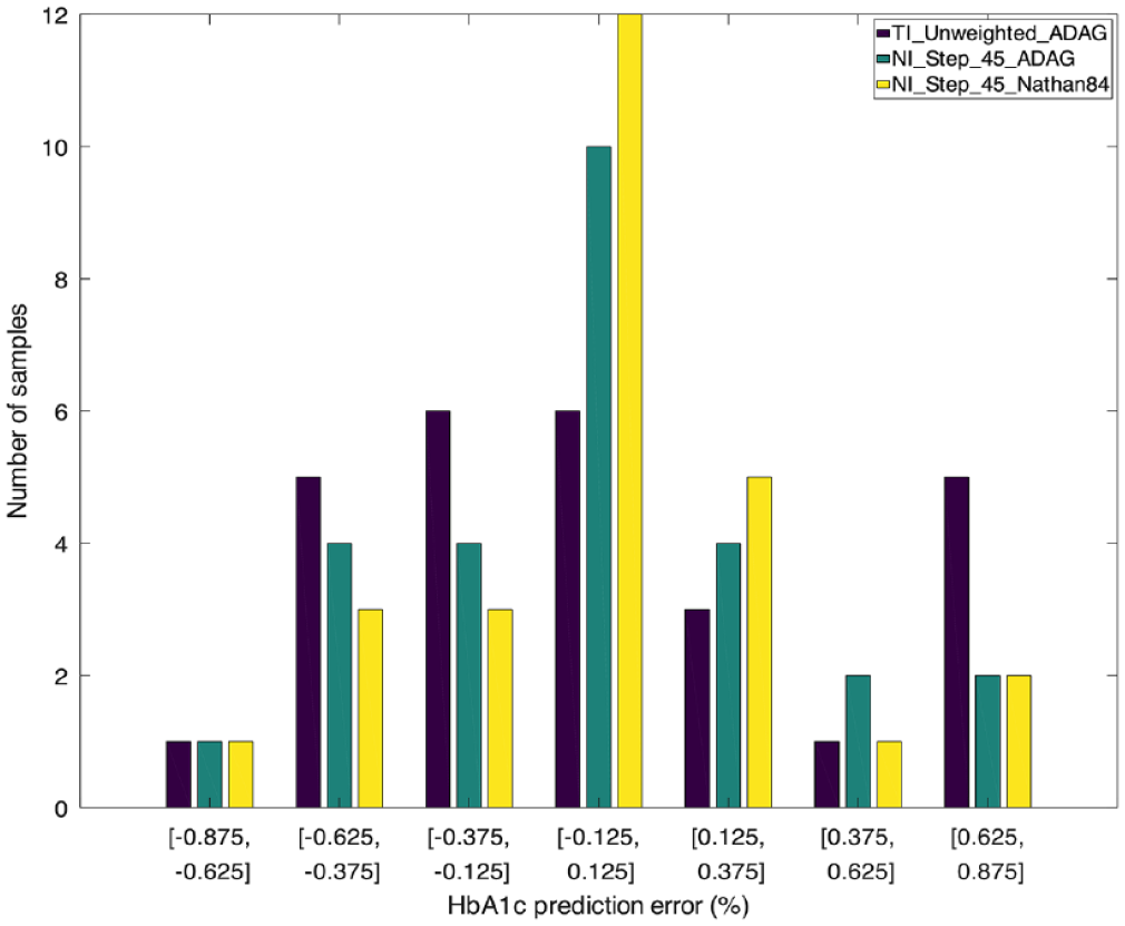
Distribution of the HbA1c prediction error of the 3 main estimation techniques considered in the study for the sample patients.

Since all methods are affected by a certain amount of bias with respect to the reference, observations have been corrected for bias before calculating the prediction error. The figure shows the histogram of the absolute, bias-corrected HbA1c prediction error, with HbA1c expressed in percent and zero-centered bins of width 0.25%.

The best estimation method found in this study (yellow bars) doubled the number of patients whose prediction error lies in the [−0.125, +0.125]% band with respect to the baseline (purple bars). The number of patients whose prediction error is higher decreased, or stayed constant, except for a slight increase (from 3 to 5 patients) in the [0.125, 0.375] band.

Another metric commonly used to compare the performance of 2 estimation techniques is to analyze their squared error with respect to the gold standard. When considering methods a and b, we obtain 2 samples of bias-compensated squared errors $E_{a}$ and $E_{b}$ , each sample consisting of one element for each observation. These 2 samples are dependent, because the underlying observations pertain to the same patients and they may not be assumed to be normally distributed.

To compare them, we chose the Wilcoxon signed-rank test²⁷ because it can be used on related samples, matched samples, or repeated observations. Moreover, it is nonparametric and does not rely on any assumption of normality.

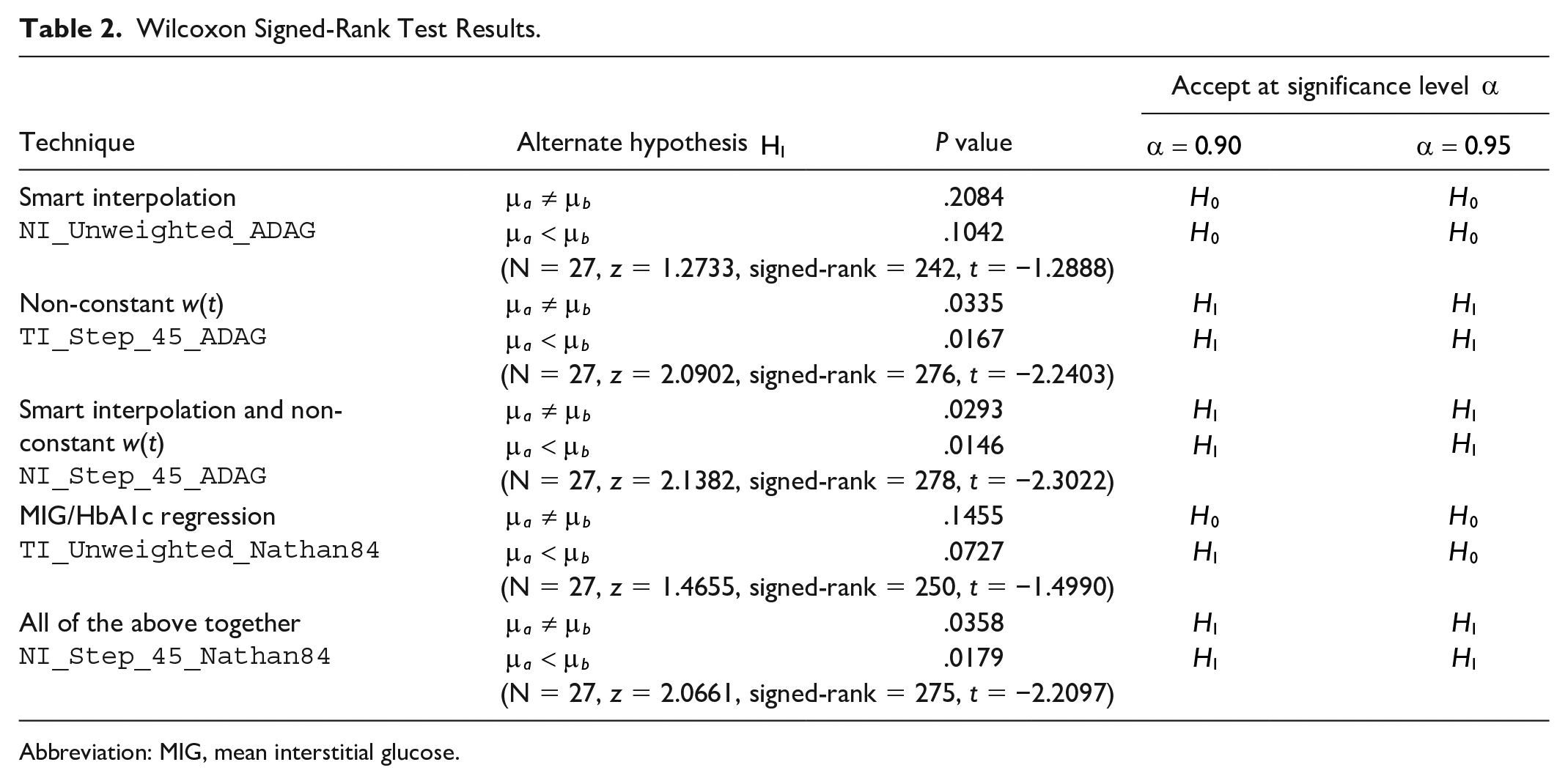
Calling $μ_{a}$ µ _a and $μ_{b}$ µ _b , the median of $E_{a}$ and $E_{b}$ , the test was applied taking as null hypothesis $H_{0} : μ_{a} = μ_{b}$ and as alternate hypothesis either $H_{1} : μ_{a} \neq μ_{b}$ (2-tailed test) or $H_{1} : μ_{a} < μ_{b}$ (1-tailed test). The alternate hypotheses test, respectively, whether the median squared error of methods a and b significantly differ, and whether a’s median square error is significantly lower (and hence, better) than b’s.

As shown in the last row of Table 2, the test revealed a significant difference in median squared error between methods NI_Step_45_Nathan84 and TI_Unweighted_ADAG (P = 0.0358, significance level α ≥ 95%) in favor of NI_Step_45_Nathan84 (P = 0.0179, significance level α ≥ 95%).

Table 2.

Wilcoxon Signed-Rank Test Results.

Technique	Alternate hypothesis $H_{1}$	P value	Accept at significance level $α$
Technique	Alternate hypothesis $H_{1}$	P value	$α = 0.90$	$α = 0.95$
Smart interpolation NI_Unweighted_ADAG	$μ_{a} \neq μ_{b}$	.2084	$H_{0}$	$H_{0}$
	$μ_{a} < μ_{b}$	.1042	$H_{0}$	$H_{0}$
	(N = 27, z = 1.2733, signed-rank = 242, t = −1.2888)
Non-constant w(t) TI_Step_45_ADAG	$μ_{a} \neq μ_{b}$	.0335	$H_{1}$	$H_{1}$
	$μ_{a} < μ_{b}$	.0167	$H_{1}$	$H_{1}$
	(N = 27, z = 2.0902, signed-rank = 276, t = −2.2403)
Smart interpolation and non-constant w(t) NI_Step_45_ADAG	$μ_{a} \neq μ_{b}$	.0293	$H_{1}$	$H_{1}$
	$μ_{a} < μ_{b}$	.0146	$H_{1}$	$H_{1}$
	(N = 27, z = 2.1382, signed-rank = 278, t = −2.3022)
MIG/HbA1c regression TI_Unweighted_Nathan84	$μ_{a} \neq μ_{b}$	.1455	$H_{0}$	$H_{0}$
	$μ_{a} < μ_{b}$	.0727	$H_{1}$	$H_{0}$
	(N = 27, z = 1.4655, signed-rank = 250, t = −1.4990)
All of the above together NI_Step_45_Nathan84	$μ_{a} \neq μ_{b}$	.0358	$H_{1}$	$H_{1}$
	$μ_{a} < μ_{b}$	.0179	$H_{1}$	$H_{1}$
	(N = 27, z = 2.0661, signed-rank = 275, t = −2.2097)

Abbreviation: MIG, mean interstitial glucose.

When analyzing the contribution to statistical significance brought by the 3 techniques considered so far (smart interpolation, non-constant w(t), and regression other than ADAG), the data in Table 2 reveal that:

The use of smart interpolation alone is insufficient to reach a statistically significant improvement.

The use of the nonconstant w(t) Step_45 alone is sufficient, at a confidence level of 95%.

Using both brings a statistically significant improvement as well.

The use of the Nathan84 instead of the ADAG regression reaches statistical significance only with a confidence level of 90% (not 95%) and only when considering the more restrictive alternate hypothesis $H_{1} : μ_{a} < μ_{b}$ .

Despite the slight decrease in the P value for NI_Step_45_Nathan84 with respect to NI_Step_45_ADAG, the use of the former is still advisable because, as shown in Table 1, it has a better adherence to HbA1c.

In all Wilcoxon signed-rank tests summarized in Table 2, no ties were observed.

Systematic errors in CGM data caused by imperfect sensor calibration can be modeled as time-variant additive and multiplicative error terms of $i g (t)$ , as proposed by Vettoretti et al,²⁸ whose effect on HbA1c estimation can in principle be assessed by incorporating these same terms in the MIG equations presented previously. However, as the error terms vary through the sensor lifetime, this leads to practical issues when the exact sensor installation and replacement dates are unknown, as it happens for the data set considered in this study. On the contrary, considering the worst-case calibration error to make the error terms time-invariant could lead to an overestimation of its effect. A more precise characterization would be possible if the CGM observation window for HbA1c estimation could be reduced to the lifespan of a single sensor. In any case, the HbA1c estimation uncertainly determined in this paper already takes the calibration error into account even without modeling it explicitly.

Finally, the accuracy of the G6 sensor has been proven to be good in several literature studies,^29,30 and this is a further element in favor of deriving satisfactory HbA1c estimates from CGM data too.

To be fair, readers should be warned that this work is far from being the final answer to the eA1C prediction problem. In fact, although it is intended to contribute in obtaining better estimates from available CGM data, a number of aspects still need further investigations and improvements. For instance, standardization and traceability of measurements data are requirements of utmost importance not only for the disease management and care but also for correct result comparisons. While traceability of HbA1c assays seems adequately established at present,³¹ the same is not true for CGM data, and differences exist not only between manufacturers but also between types of sensors by the same manufacturer.³²

Among others, this makes the comparison of estimation techniques difficult when, in general, they are carried out in different operating conditions. Prediction improvements shown by our study are consistent (and methods fairly comparable) because a single type of sensor was used and the various computation alternative were applied to the same CGM data set. Then obtained results are significant but in a relative way (eg, NI_Step_45_Nathan84 performs surely better than TI_Unweighted_ADAG), while absolute figures might not (and likely would not) be the same if a different type or multiple types or sensors were used.

Conclusions

While CGM-derived metrics (eg, TiR and TaR) are becoming more and more popular in diabetes care, HbA1c is still the gold standard and most healthcare professionals are accustomed to its use as a reference parameter. Thus, the estimation of HbA1c from CGM plays the important role of enabling a smooth and increasing coaching of CGM in diabetes care,³³ by effectively relating its metrics to the well-consolidated use of HbA1c.

Evaluating HbA1c quickly, precisely, and reliably from CGM data without resorting to laboratory assays can bring considerable benefits to both diabetologists and patients, besides reducing care times and costs for public health systems. These benefits could be obtained not only through a reduction of HbA1c,³⁴ but also in the routine monitoring of patients’ health by suitably reducing the number or yearly assays.³⁵ This study has shown how the adoption of a patching strategy for CGM data acquired in real-life conditions and the selection of a suitable weighting function and regression equation in the data processing chain contribute to reduce the variance of the eA1C-HbA1c differences by about 38% with respect to other published solutions.

Improvements obtained by selecting different patching strategies, weighting functions and regression equations have been compared through both BA plots and the Wilcoxon signed-rank test on the squared error with respect to HbA1c.

The advantages discussed in this paper can be achieved through the direct introduction of the proposed techniques in commercial CGM devices and data processing software, with very little effort and cost. Their adoption would bring benefits to both clinicians and patients in their everyday monitoring routine besides strengthening their confidence in eA1C (or GMI) predictions. The study has also shown that acting on a single factor at a time (eg, the regression equation) as done in some previous studies is unlikely to produce considerable practical benefits.

Supplemental Material

sj-docx-1-dst-10.1177_19322968221081556 – Supplemental material for Predicting Glycated Hemoglobin Through Continuous Glucose Monitoring in Real-Life Conditions: Improved Estimation Methods

Supplemental material, sj-docx-1-dst-10.1177_19322968221081556 for Predicting Glycated Hemoglobin Through Continuous Glucose Monitoring in Real-Life Conditions: Improved Estimation Methods by Marina Valenzano, Ivan Cibrario Bertolotti, Giorgio Grassi, Fabio Broglio and Adriano Valenzano in Journal of Diabetes Science and Technology

Footnotes

Acknowledgements

The School of Endocrinology and Metabolic Diseases of the University of Torino and the Ospedale Molinette di Torino supported the observation, monitoring and follow-up of patients in this study. The Institute of Electronics, Information Engineering and Telecommunications of the National Research Council of Italy supported the data processing, mathematical and statistical analysis.

Author’s Note

Marina Valenzano is now affiliated to Territorial Department of Diabetology and Endocrinology - Local Health Authority Cuneo 1 (ASL CN1), Cuneo, Italy.

Abbreviations

(CGM) continuous glucose monitoring, (RT-CGM) real-time continuous glucose monitoring, (HbA1c) glycated hemoglobin, (eA1C) estimated glycated hemoglobin, (BA) Bland-Altman, (IG) interstitial glucose, (MIG) mean interstitial glucose, (MSE) mean squared error, (GMI) glucose management indicator, (AUC) area under curve, (BMI) body mass index, (HPLC) high-performance liquid chromatography, (REALISM-T1D) real-life glucose monitoring in type 1 diabetes, (ADAG) A1C-derived average glucose, (UKPDS) United Kingdom prospective diabetes study, (DCCT) diabetes control and complications trial, (CI) confidence interval, (QQ) quartile-quartile, (AD) Anderson-Darling.

Author Contributions

All authors evenly participated in the design of the study. Marina Valenzano, Giorgio Grassi and Fabio Broglio took care of patient follow-up, also supervising all visits. Ivan Cibrario Bertolotti and Adriano Valenzano performed the relevant data processing and statistical analysis. All authors contributed significantly to the writing and editing process of this manuscript.

Declaration of Conflicting Interests

The author(s) declared no potential conflicts of interest with respect to the research, authorship, and/or publication of this article.

Funding

The author(s) received no financial support for the research, authorship, and/or publication of this article.

Ethics Approval

The Joint Ethics Committee “A. O. Città della Salute e della Scienza di Torino, A.O. Ordine Mauriziano, A.S.L. Città di Torino” approved this study (rec. number 0029846).

ORCID iDs

Marina Valenzano

Ivan Cibrario Bertolotti

Adriano Valenzano

References

Little

Rohlfing

. HbA1c standardization: background, progress and current issues. Lab Med. 2009;40(6):368-373.

Hanas

John

International HbA1c Consensus Committee. 2013 update on the worldwide standardization of the hemoglobin A1c measurement. Clin Chem LabMed. 2013;51(5):1041-1042.

Ribet

Stemme

Roxhed

. Real-time intradermal continuous glucose monitoring using a minimally invasive microneedle-based system. Biomed Microdevices. 2018;20:101.

Nathan

Kuenen

Borg

Zheng

Schoenfeld

Heine

. Translating the A1C assay into estimated average glucose values. Diabetes Care. 2008;31:1473-1478.

Bergenstal

Beck

, et al. Glucose Management Indicator (GMI): a new term for estimating A1C, from continuous glucose monitoring. Diabetes Care. 2018;41(11):2275-2280.

Nathan

Turgeon

Regan

. Relationship between glycated haemoglobin levels and mean glucose levels over time. Diabetologia. 2007;50:2239-2244.

Shen

Yan

, et al. Relationship between estimated glycosylated hemoglobin using flash glucose monitoring and actual measured glycosylated hemoglobin in a Chinese population. Diabetes Ther. 2019;11:2027.

Rohlfing

Wiedmeyer

Little

England

Tennill

Goldstein

. Defining the relationship between plasma glucose and HbA(1c): analysis of glucose profiles and HbA(1c) in the Diabetes Control and Complications Trial. Diabetes Care. 2001;25:275-278.

Inoue

Goto

Kishimoto

, et al. Possible discrepancy of HbA1c values and its assessment among patients with chronic renal failure, hemodialysis and other diseases. Clin Exp Nephrol. 2015;19:1179-1183.

10.

Perlman

Gooley

McNulty

, et al. HbA1c and glucose management indicator discordance: a real-world analysis. Diabetes Technol Ther. 2021;23(4):253-258.

11.

Ramchandani

Arya

Ten

, et al. Real-life utilization of real-time continuous glucose monitoring: the complete picture. J Diabetes Sci Technol. 2011;5(4):860-870.

12.

Fonda

Lewis

Vigersky

. Minding the gaps in continuous glucose monitoring: a method to repair gaps to achieve more accurate glucometrics. J Diabetes Sci Technol. 2013;7(1):88-92.

13.

Leow

MKS

. Glycated hemoglobin (HbA1c): clinical applications of a mathematical concept. Acta Inform Med. 2016;24:233-238.

14.

UK Prospective Diabetes Study (UKPDS) Group: intensive blood-glucose control with sulphonylureas or insulin compared with conventional treatment and risk of complications in patients with type 2 diabetes (UKPDS 33). Lancet. 1998;352:837-853.

15.

The DCCT research group: Diabetes Control and Complications Trial (DCCT): results of feasibility study. Diabetes Care. 1987;10(1):101.

16.

Nathan

Singer

Hurxthal

Goodson

. The clinical information value of the glycosylated hemoglobin assay. N Engl J Med. 1984;310:341-346.

17.

Divine

Norton

Hunt

Dienemann

. A review of analysis and sample size calculation considerations for wilcoxon tests. Anesth Analg. 2013;117(3):699-710.

18.

Malviya

Bansal

Pal

, et al. High performance liquid chromatography: a short review. J Glob Pharma Technol. 2010;2(5):22-26.

19.

Enders

. Applied Missing Data Analysis. New York, NY: Guilford Press; 2010.

20.

Mortensen

Vølund

. Application of a biokinetic model for prediction and assessment of glycated haemoglobins in diabetic patients. Scand J Clin Lab Invest. 1988;48:595-602.

21.

Tahara

Shima

. The response of GHb to stepwise plasma glucose change over time in diabetic patients. Diabetes Care. 1993;16:1313-1314.

22.

DelRio

Tiwari

Amodu

Cagliani

Rilo

HLR

. Glycated hemoglobin, plasma glucose, and erythrocyte aging. J Diabetes Sci Technol. 2016;10:1303-1307.

23.

Bland

Altman

. Measuring agreement in method comparison studies. Stat Methods Med Res. 1999;8:135-160.

24.

Giavarina

. Understanding bland altman analysis. Biochem Med. 2015;25:141-151.

25.

Anderson

Darling

. Asymptotic theory of certain goodness of fit criteria based on stochastic processes. Ann Math Stat. 1952;23(2):193-212.

26.

Stephens

. EDF statistics for goodness of fit and some comparisons. J Am Stat Assoc. 1974;69:730-737.

27.

Wilcoxon

. Individual comparisons by ranking methods. Biometrics Bull. 1945;1:80-83.

28.

Vettoretti

Del Favero

Sparacino

Facchinetti

. Modeling the error of factory-calibrated continuous glucose monitoring sensors: application to Dexcom G6 sensor data. 41st Annual International Conference of the IEEE Engineering in Medicine and Biology Society (EMBC). 2019;2019:750-753.

29.

Wadwa

Laffel

Shah

Garg

. Accuracy of a factory-calibrated, real-time continuous glucose monitoring system during 10 days of use in youth and adults with diabetes. Diabetes Technol Ther. 2018;20(6):395-402.

30.

Shah

Laffel

Wadwa

Garg

. Continuous glucose monitoring system utilizing an automated sensor applicator. Diabetes Technol Ther. 2018; 20(6):428-433.

31.

Panteghini

John

. Implementation of haemoglobin A1c results traceable to the IFCC reference system: the way forward. Clin Chem Lab Med. 2007;45(8):942-944.

32.

Freckmann

Nichols

Hinzmann

, et al. Standardization process of continuous glucose monitoring: traceability and performance. Clinical Chimica Acta. 2021;515:5-12.

33.

Heinemann

Freckmann

Muller-Wieland

, et al. Critical reappraisal of the time-in-range: alternative or useful addition to glycated hemoglobin? J Diabetes Sci Technol. 2020;14(5):922-927.

34.

Bansal

Shah

Reilly

, et al. Impact of reducing glycated hemoglobin on healthcare costs among a population with uncontrolled diabetes. Appl Health Econ Health Policy. 2018;16:675-684.

35.

Chadee

Blackhouse

Goeree

. Point-of-care hemoglobin A1c testing: a budget impact analysis. Ont Health Technol Assess Ser. 2014;14(9):1-23.

Supplementary Material

Please find the following supplemental material available below.

For Open Access articles published under a Creative Commons License, all supplemental material carries the same license as the article it is associated with.

For non-Open Access articles published, all supplemental material carries a non-exclusive license, and permission requests for re-use of supplemental material or any part of supplemental material shall be sent directly to the copyright owner as specified in the copyright notice associated with the article.

0.00 MB

0.05 MB