Sage Journals: Discover world-class research

Abstract

Background:

Abnormal glucose variability (GV) is a risk factor for diabetes complications, and tens of indices for its quantification from continuous glucose monitoring (CGM) time series have been proposed. However, the information carried by these indices is redundant, and a parsimonious description of GV can be obtained through sparse principal component analysis (SPCA). We have recently shown that a set of 10 metrics selected by SPCA is able to describe more than 60% of the variance of 25 GV indicators in type 1 diabetes (T1D). Here, we want to extend the application of SPCA to type 2 diabetes (T2D).

Methods:

A data set of CGM time series collected in 13 T2D subjects was considered. The 25 GV indices considered for T1D were evaluated. SPCA was used to select a subset of indices able to describe the majority of the original variance.

Results:

A subset of 10 indicators was selected and allowed to describe 83% of the variance of the original pool of 25 indices. Four metrics sufficient to describe 67% of the original variance turned out to be shared by the parsimonious sets of indices in T1D and T2D.

Conclusions:

Starting from a pool of 25 indices assessed from CGM time series in T2D subjects, reduced subsets of metrics virtually providing the same information content can be determined by SPCA. The fact that these indices also appear in the parsimonious description of GV in T1D may indicate that they could be particularly informative of GV in diabetes, regardless of the specific type of disease.

Keywords

continuous glucose monitoring glucose variability type 1 diabetes type 2 diabetes

The likely effect of glucose variability (GV) on the increased risk of complications in diabetes^1-6 has pushed researchers to propose a number of indices that can be used to quantify GV from either self-monitoring blood glucose (SMBG) or continuous glucose monitoring (CGM) time series. CGM profiles, in particular, because of their capability to capture components of glucose dynamic invisible even in the full 7-point SMBG profiles, are powerful tools to be exploited for the retrospective assessment of GV. Indices for GV quantification proposed in the literature include metrics quantifying the dispersion of glucose readings, the amplitude of glucose fluctuations, the risk of extreme glucose conditions (ie, hypo- and hyperglycemia), and the overall quality of glycemic control. We refer the reader to other sources^7-11 for recent reviews. In this pool of available GV indices, however, several metrics have similar formulations or measure almost the same physiological quantity, with highly redundant information in the characterization of GV. Thus, a method capable of extracting a reduced subset of metrics still effective for describing GV in a specific population would be desirable.

In a recent work,¹² we have proposed the use of sparse principal component analysis (SPCA)—a technique introduced by Zou et al¹³—as an approach to select a subset of GV indices from a wider pool of metrics and provide a parsimonious description of GV in type 1 diabetes (T1D). As detailed in Fabris et al,¹² SPCA extracts a combination of a reduced number of GV indices that together preserve the majority of the variance of the initial wider pool of metrics; in terms of variance, GV indicators selected by SPCA are able to convey and reconstruct almost the whole information expressed by the original set of indices. In our previous work,¹² SPCA was successfully applied to a data set of CGM time series collected in 33 T1D subjects, selecting a reduced number of up to 10 GV indices able to span more than 60% of the original variance. The aim of the present article is to extend the application of SPCA to type 2 diabetes (T2D).

Materials and Methods

Database

The data set consists of CGM time series collected from 13 T2D males for an average period of 6 days under normal life conditions using the Medtronic® Guardian REAL-Time® CGM System (Medtronic, Northridge, CA). Mean ± SD demographic information of the data set is age, 54.4 ± 10.0 years; duration of diabetes, 10.7 ± 7.0 years; glycosylated hemoglobin, 7.4 ± 1.4 %; and body mass index, 29.4 ± 3.6 kg/m².

The Original Pool of GV Indices

Twenty-five well-established indices for GV quantification were considered similarly to Fabris et al.¹² The pool of metrics includes mean and sample standard deviation (SD) of all glucose readings, percentage coefficient of variation (%CV), mean of daily SDs (SD_w), SD of daily means (SD_dm), J-index (a combination of mean and SD),¹⁴ percentages of values below, within and above the euglycemic target range (70-180 mg/dl), 50^th percentile, interquartile range (IQR), range of glucose readings, and the mean amplitude of glycemic excursions (MAGE) index.^15,16 Moreover, measures derived from nonlinear transformations of glucose values quantifying the risk associated to a glucose profile were also evaluated: we considered low and high blood glucose indices (LBGI, HBGI),^17,18 average daily risk range (ADRR),¹⁹ and blood glucose risk index (BGRI);¹¹ hyperglycemic index, hypoglycemic index, and index of glycemic control (IGC);⁸ the glycemic risk assessment diabetes equation (GRADE) score and the 3 contributions due to the different glycemic states, that is, %GRADEhypo, %GRADEeu, %GRADEhyper;²⁰ and, finally, the M₁₀₀ index.²¹ For all these indices, hypo and hyperglycemic thresholds, when appropriate, were set at 70 and 180 mg/dl, respectively.

The listed GV indices were evaluated on the CGM time series of the data set under analysis (the correlation matrix of the 25 metrics in the considered T2D population is reported in the Appendix to this paper). Then, before entering SPCA, each GV index was mean centered and scaled (ie, divided by its sample SD) to avoid any bias in the SPCA results and to facilitate the comparison of results obtained from different data sets.¹²

SPCA

SPCA is a 2-step data processing technique of general applicability introduced by Zou et al.¹³ Details on the implementation for our purposes can be found in Fabris et al¹²; here, we report only a brief description.

Let X be the n x m data matrix collecting the m GV indices evaluated on the n CGM profiles (of n different subjects) of the data set under analysis. The 2 steps of SPCA are:

Step (a): apply the principal component analysis (PCA) technique²² to the matrix X to retrieve the principal components (PCs), and select a reduced number p (p<<m) of them, saving the majority of the total original variance (of note is that, when n<m, only the first n PCs, as associated to nonzero eigenvalues, can be meaningful in the analysis, and the number of selected PCs must satisfy the constraint p<n). As in Fabris et al,¹² the number of selected PCs was determined so that at least 85% of the total original variance was saved after the PCA step, with p being the minimum number of PCs that could preserve this percentage. Additional PCs were added to the set only if the percentage of saved variance was further increased of at least 10%. This is in line with the principle of parsimony: the higher the number of PCs, the higher the number of finally selected GV indices; thus, the benefit in terms of explained variance has to be significant.

Step (b): apply the least absolute shrinkage and selection operator (LASSO) constraint²³ to each selected PC to obtain sparse estimates of regression coefficients and maintain in the PC regressor a reduced number of GV indices. Since PCs are linear combinations (regressions) of all the original variables, this will reduce the number of explicitly considered GV indices for each PC, still preserving a high percentage of the total original variance. The number of nonzero coefficients for each PC was determined so that the selected subset was of the same size as the one obtained in our previous work,¹² that is, we selected 5 GV indices for each PC, to get a final subset of 10 metrics.

Calculation of GV indices and implementation of SPCA were performed with software developed by us in MATLAB® environment.

Results

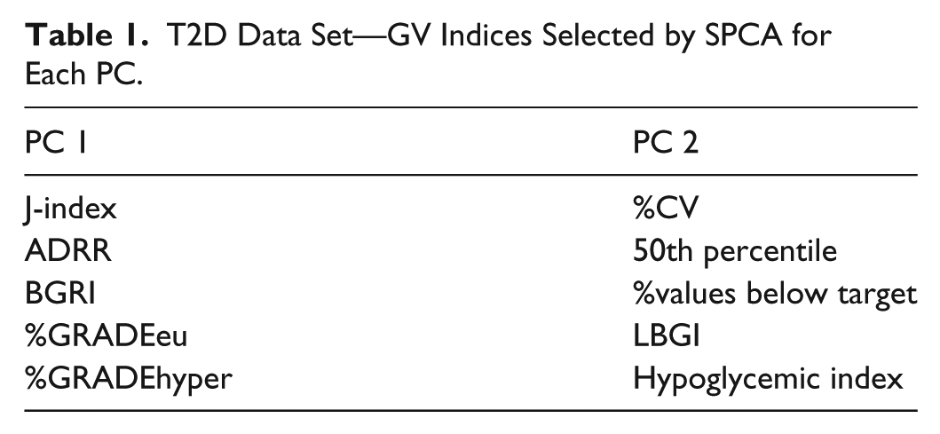
The m = 25 GV indices were evaluated on the n = 13 CGM profiles of the T2D data set, and SPCA was subsequently applied. The first step of SPCA led to the selection of 2 out of 25 PCs, since with 2 PCs it was possible to go beyond the defined 85% threshold and preserve 88% of the original variance. This can be seen from the top-left panel of Figure 1, where the percentage explained variance is plotted as a function of the number of selected PCs for the T2D data set; the horizontal red line in the figure is the threshold at 85%. The reduction of data dimensionality from 25 to 2 achieved through PCA suggests that, if analyzed in terms of PCs, GV is mainly a 2-dimensional phenomenon. PCs, however, are not GV indices, but combinations of several indicators, and interpreting them in terms of physiological meaning is difficult. Thus, to move the problem back to the GV domain, the LASSO step was performed. The trend of the percentage explained variance as a function of the number of GV indices selected per PC is shown in the right panel of Figure 1. From the plot, it can be seen that with a pool of indices of the same dimension as that selected for the T1D data set, that is, made up of 10 metrics, the variance preserved for the T2D data set was equal to 83% of the total original one. For this specific data set, however, an even smaller subset of indices was sufficient to cross the 60% threshold of explained variance, given that 2 GV indices per PC allowed to explain 67% of the original variance. The parsimonious set of GV indices selected by SPCA is reported in Table 1. The table shows the 10-index pool (5 indices for each PC), and the smaller pool of 4 metrics, that is a subset of the former, is made up of the indicators that appear as underlined.

Figure 1.

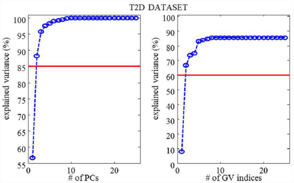
T2D data set—percentage explained variance as a function of selected PCs (left panel) and selected GV indices per PC (right panel).

Table 1.

T2D Data Set—GV Indices Selected by SPCA for Each PC.

PC 1	PC 2
J-index	%CV
ADRR	50th percentile
BGRI	%values below target
%GRADEeu	LBGI
%GRADEhyper	Hypoglycemic index

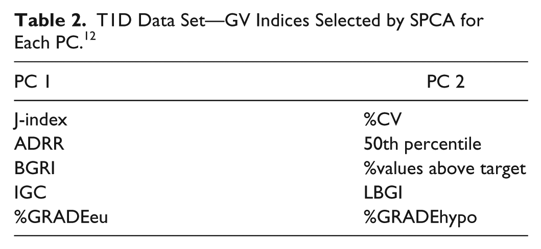
These results obtained in T2D are in line with those reported in Fabris et al,¹² where SPCA was applied to the same 25 GV indicators, evaluated on 33 CGM time series acquired from T1D subjects monitored for 4 days using the Dexcom® SEVEN® Plus CGM System (Dexcom, San Diego, CA, USA). To help the reader in the comparison, we report the plots used for the choice of SPCA parameters in Figure 2 and the set of indices finally selected in Table 2. Two out of 25 PCs were selected also for the T1D data set and 5 GV indices per PC were necessary to save more than 60% of the original variance (62% was finally saved). Interestingly, the 4 GV indices selected for the T2D data set are all included in the T1D parsimonious set, seeming to be particularly informative of GV in diabetes, regardless of the specific type of disease.

Figure 2.

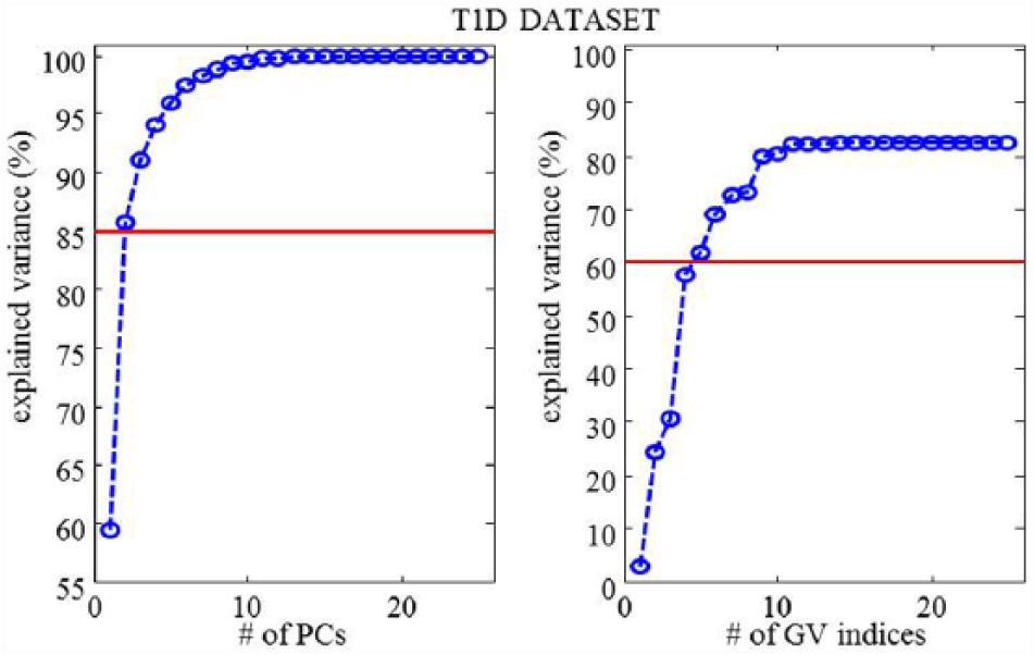
T1D data set—percentage explained variance as a function of selected PCs (left panels) and selected GV indices per PC (right panels).

Table 2.

T1D Data Set—GV Indices Selected by SPCA for Each PC.¹²

PC 1	PC 2
J-index	%CV
ADRR	50th percentile
BGRI	%values above target
IGC	LBGI
%GRADEeu	%GRADEhypo

Discussion

Robustness of SPCA Results

In the previous section, results obtained from the application of SPCA to 25 GV indicators evaluated on 13 T2D CGM time series have been documented. Nevertheless, no information has been provided about the robustness of what was achieved. This section will discuss this aspect, investigating if and how measurement noise and the low sample size data context that we have (less CGM signals than GV indices) influence the obtained results.

SPCA robustness to measurement noise can be theoretically proved by observing the intrinsic robustness to noise of PCA, which is indeed widely used in denoising applications. As detailed in Fabris et al¹² and mentioned in Section 2.3, PCs obtained from PCA are sorted by the amplitude of the covariance matrix eigenvalues. This means that the first PCs, as associated to the largest eigenvalues, are the most significant, while other PCs associated to small eigenvalues account mostly for noise. Selecting the first PCs allows to filter the noise affecting the data, and this is what we achieved in our application by selecting 2 out of 25 PCs. Beyond this intrinsic robustness to noise of PCA, to further prove that SPCA does not respond to noise, we performed 3 different perturbations of the original data set SPCA was computed on. Given that a direct perturbation of GV indices was not possible because of the correlation among them, we achieved variations of their values through a perturbation of the original (independent) CGM signals. Specifically, we (1) smoothed the CGM time series using a Savitzky–Golay filter, (2) added white noise with zero mean and 5% SD to the original CGMs, and (3) added white noise with zero mean and 10% SD to them. In all 3 scenarios, we got exactly the same results, with the same 10 GV indices selected and 83% of the original variance saved, confirming the robustness of SPCA to intrinsic or additional noise in our data.

The second technical aspect that deserves a discussion is the consistency of PCA, that is, the precision in estimating the PC coefficients, given the small number of available observations (n = 13) as compared with the number GV indices (m = 25). To deal with this issue, we referred to some recent literature findings,^24-26 where sample PCA (through the eigen-decomposition of the sample covariance matrix) was proved to be still well-defined with m>n, and tested the robustness of SPCA results to small perturbations of the original data set. Specifically, we removed 1 CGM signal from the initial data set and saw how results varied with respect to the original ones as the removed time series changed. Specifically, we could perform SPCA 13 times, each time having a 12 time series data set. Results obtained from this analysis were more than satisfactory since we had (1) 1 scenario where exactly the same results (same subset of 10 selected indices) were achieved, (2) 8 scenarios where 1 (out of 10) selected parameter was different (%GRADEhyper was replaced or deleted 7 times from the first PC, Hypo Index was deleted 1 time from the second PC), (3) 2 scenarios where 2 (out of 10) selected parameters were different, (4) 2 scenarios where 5 (out of 10) selected parameters were different. In all cases, 78% or more of the original variance was saved. From these results we can see that PCs/sparse PCs seem to be robustly estimated and consistent to slight changes of the original data set. Of note is also that parameters that are replaced or removed from the original 10-index pool are those corresponding to smaller coefficients within each sparse regressor, thus contributing less than the others to the final explained variance. Beyond this analysis, however, we still need a larger number of CGM time series to finally select a subset of indicators which is actually the most representative of GV in diabetes. When larger data sets representative of the whole diabetic population will become available, the pool of GV indices will be enlarged including all literature metrics, and a more solid subset of the most representative GV indices in T1D and T2D will be identified via SPCA. At the present time, a significant increase of the number of variables is unfeasible because, as discussed, it could lead to inconsistency in the estimation of PCs/sparse PCs.

Clinical Interpretation of SPCA Results

SPCA results need also to be considered from a clinical viewpoint. Specifically, as already seen in Fabris et al,¹² we can observe from this analysis that GV can be reduced to a 2-dimensional phenomenon, well described by 2 combinations of indicators (either PCs or sparse PCs) identified through SPCA. A clinical interpretation of the meaning of each PC/sparse PC is not trivial, but we can observe that the first sparse PC, that is, the one describing the largest part of the variance of the original pool of GV indices, is mainly influenced by glucose control and hyperglycemia indices, while the second one, less significant in terms of variance than the first one, but still meaningful, accounts for hypoglycemia. This seems reasonable because hyperglycemic conditions may be more varying from 1 patient to the other than hypoglycemic ones, given the larger amplitude of the hyperglycemic range and the consequent much wider range of possible hyperglycemic scenarios. Of note is that the independence between the 2 PCs allows to capture and characterize the 2 extreme glycemic conditions separately.

Starting from the result that GV can be considered as a 2-dimensional phenomenon described by the first 2 PCs/sparse PCs, a clinically relevant usefulness of SPCA and its outputs can take shape. Specifically, the next step will consist in investigating if PCs and sparse PCs can be used for classification purposes, for example, to discriminate between groups of subjects affected by different metabolic disorders and between patients having different levels of quality of glycemic control. The development of a classifier based on PCs and sparse PCs is currently being conducted and preliminary results are promising.

Conclusions

GV is a risk factor for the development of complications from diabetes and tens of indicators for its quantification from CGM signals have been proposed in the literature. Despite the large number of available GV indices, a gold-standard metric to assess GV has not been identified yet, and a combination of indices is very likely to be needed to reliably characterize GV from glucose profiles.^27,28 However, because some indices have similar mathematical formulations or measure almost the same physiological entity, considering all available GV metrics will provide highly redundant information and some indices could be of limited added value in the characterization of GV within a diabetic population. In this context, we have recently proposed a SPCA-based approach to select, from a pool of m = 25 GV indices, a reduced set of metrics able to parsimoniously describe GV in T1D by preserving the majority of the variance originally present in the data.¹² In this work, we have extended the application of SPCA to T2D. Specifically, the same m = 25 GV indices considered in Fabris et al¹² were evaluated on a 13 T2D subject CGM data set. With a selected pool of 10 indicators, that is, of the same size as that selected in Fabris et al¹² for T1D, 83% of the original variance was described. Moreover, for this specific T2D data set, a reduced pool of 4 indices, namely, J-index, %GRADEeu, %CV, and LBGI, was already sufficient to save 67% of the variance. It is worth recalling that, for the T1D data set considered in Fabris et al,¹² the indicators selected by SPCA were J-index, ADRR, BGRI, IGC, %GRADEeu, %CV, 50^th percentile, %values above target, LBGI, and %GRADEhypo, saving 62% of the original variance of the indicators; therefore, the 4 indices selected by SPCA for the T2D data set are all included in the parsimonious T1D set. This finding suggests that such a small group of indices could be regarded as particularly informative of GV in diabetes, and SPCA seems to be the proper tool to identify it. However, results obtained so far do not allow to state that these 4 GV metrics can be considered as a gold-standard subset representative of GV in diabetes yet. In fact, any definitive conclusion should consider a much richer pool of GV indices, including, for example, the continuous overlapping net glycemic action,²⁹ the mean of daily differences,³⁰ the lability index,³¹ and new indices based on the dynamic risk concept,³² and a large number of CGM time series. Beyond the extension of data set and initial pool of metrics, future developments of this study will include investigating more technical aspects related to SPCA, for example, the clinical interpretation of PCs/sparse PCs and the role played by the selected GV indices within each of them, and exploiting the use of SPCA and its outcomes to manage classification problems of subjects with different metabolic disorders.

Footnotes

Appendix

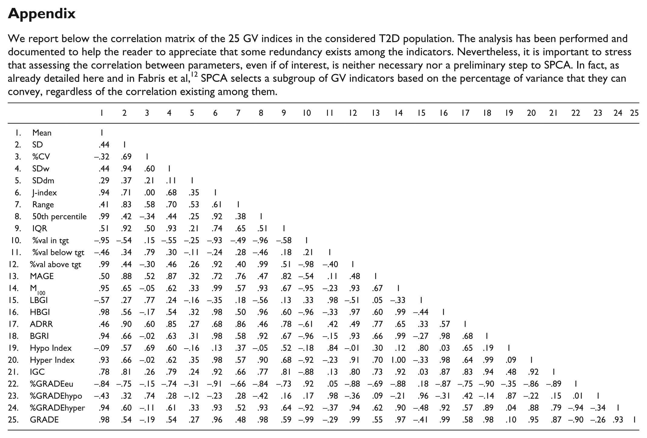
We report below the correlation matrix of the 25 GV indices in the considered T2D population. The analysis has been performed and documented to help the reader to appreciate that some redundancy exists among the indicators. Nevertheless, it is important to stress that assessing the correlation between parameters, even if of interest, is neither necessary nor a preliminary step to SPCA. In fact, as already detailed here and in Fabris et al,¹² SPCA selects a subgroup of GV indicators based on the percentage of variance that they can convey, regardless of the correlation existing among them.

	1	2	3	4	5	6	7	8	9	10	11	12	13	14	15	16	17	18	19	20	21	22	23	24	25
1. Mean	1
2. SD	.44	1
3. %CV	–.32	.69	1
4. SDw	.44	.94	.60	1
5. SDdm	.29	.37	.21	.11	1
6. J-index	.94	.71	.00	.68	.35	1
7. Range	.41	.83	.58	.70	.53	.61	1
8. 50th percentile	.99	.42	–.34	.44	.25	.92	.38	1
9. IQR	.51	.92	.50	.93	.21	.74	.65	.51	1
10. %val in tgt	–.95	–.54	.15	–.55	–.25	–.93	–.49	–.96	–.58	1
11. %val below tgt	–.46	.34	.79	.30	–.11	–.24	.28	–.46	.18	.21	1
12. %val above tgt	.99	.44	–.30	.46	.26	.92	.40	.99	.51	–.98	–.40	1
13. MAGE	.50	.88	.52	.87	.32	.72	.76	.47	.82	–.54	.11	.48	1
14. M₁₀₀	.95	.65	–.05	.62	.33	.99	.57	.93	.67	–.95	–.23	.93	.67	1
15. LBGI	–.57	.27	.77	.24	–.16	–.35	.18	–.56	.13	.33	.98	–.51	.05	–.33	1
16. HBGI	.98	.56	–.17	.54	.32	.98	.50	.96	.60	–.96	–.33	.97	.60	.99	–.44	1
17. ADRR	.46	.90	.60	.85	.27	.68	.86	.46	.78	–.61	.42	.49	.77	.65	.33	.57	1
18. BGRI	.94	.66	–.02	.63	.31	.98	.58	.92	.67	–.96	–.15	.93	.66	.99	–.27	.98	.68	1
19. Hypo Index	–.09	.57	.69	.60	–.16	.13	.37	–.05	.52	–.18	.84	–.01	.30	.12	.80	.03	.65	.19	1
20. Hyper Index	.93	.66	–.02	.62	.35	.98	.57	.90	.68	–.92	–.23	.91	.70	1.00	–.33	.98	.64	.99	.09	1
21. IGC	.78	.81	.26	.79	.24	.92	.66	.77	.81	–.88	.13	.80	.73	.92	.03	.87	.83	.94	.48	.92	1
22. %GRADEeu	–.84	–.75	–.15	–.74	–.31	–.91	–.66	–.84	–.73	.92	.05	–.88	–.69	–.88	.18	–.87	–.75	–.90	–.35	–.86	–.89	1
23. %GRADEhypo	–.43	.32	.74	.28	–.12	–.23	.28	–.42	.16	.17	.98	–.36	.09	–.21	.96	–.31	.42	–.14	.87	–.22	.15	.01	1
24. %GRADEhyper	.94	.60	–.11	.61	.33	.93	.52	.93	.64	–.92	–.37	.94	.62	.90	–.48	.92	.57	.89	.04	.88	.79	–.94	–.34	1
25. GRADE	.98	.54	–.19	.54	.27	.96	.48	.98	.59	–.99	–.29	.99	.55	.97	–.41	.99	.58	.98	.10	.95	.87	–.90	–.26	.93	1

Acknowledgements

CGM data were kindly provided by Alberto Maran (University of Padova, Padova, Italy) for T1D and by Alejandra Guillén (Medtronic Iberica, Madrid, Spain), Giuseppe Fico, and Maria Teresa Arredondo for T2D, data collected within the framework of METABO, a research project funded by EU (grant agreement FP7-216270).

Abbreviations

ADRR, average daily risk range; BGRI, blood glucose risk index; CGM, continuous glucose monitoring; CV, coefficient of variation; GRADE, glycemic risk assessment diabetes equation; %GRADEhypo/eu/hyper, percentages of GRADE due to hypo/eu/hyperglycemia; GV, glucose variability; HBGI, high blood glucose index; IGC, index of glycemic control; IQR, interquartile range; LASSO, least absolute shrinkage and selection operator; LBGI, low blood glucose index; MAGE, mean amplitude of glycemic excursions; PC, principal component; PCA, principal component analysis; SD, standard deviation; SD_dm, SD between daily means; SD_w, SD within day; SPCA, sparse principal component analysis; T1D, type 1 diabetes; T2D, type 2 diabetes.

Declaration of Conflicting Interests

The author(s) declared no potential conflicts of interest with respect to the research, authorship, and/or publication of this article.

Funding

The author(s) disclosed receipt of the following financial support for the research, authorship, and/or publication of this article: The MOSAIC project was funded by the EU within the 7th Framework Program (grant agreement FP7-600914)

References

Diabetes Control and Complications Trial (DCCT) Research Group. The effect of intensive treatment of diabetes on the development and progression of long-term complications in insulin dependent diabetes mellitus. N Engl J Med. 1993;329:977-986.

Hirsch

. Glycemic variability: it’s not just A1c anymore! Diabetes Technol Ther. 2005;7:780-783.

Hirsch

Brownlee

. Should minimal blood glucose variability become the gold standard of glycemic control? J Diabetes Complications. 2005;19:178-181.

Brownlee

Hirsch

. Glycemic variability: a hemoglobin A1c-independent risk factor for diabetes complications. JAMA. 2006;295:1707-1708.

Monnier

Mas

Ginet

Michel

Villon

Cristol

Colette

. Activation of oxidative stress by acute glucose fluctuations compared with sustained chronic hyperglycemia in patients with type 2 diabetes. JAMA. 2006;295:1681-1687.

Soupal

Skrha

Jr Fajmon

. Glycemic variability is higher in type 1 diabetes patients with microvascular complications irrespective of glycemic control. Diabetes Technol Ther. 2014;16:198-203.

Rodbard

. New and improved methods to characterize glycemic variability using continuous glucose monitoring. Diabetes Technol Ther. 2009;11:551-565.

Rodbard

. Interpretation of continuous glucose monitoring data: glycemic variability and quality of glycemic control. Diabetes Technol Ther. 2009;11:S55-S67.

Rodbard

Bailey

Jovanovic

Zisser

Kaplan

Garg

. Improved quality of glycemic control and reduced glycemic variability with use of continuous glucose monitoring. Diabetes Technol Ther. 2009;11:717-723.

10.

Rodbard

. Glycemic variability: measurement and utility in clinical medicine and research—one viewpoint. Diabetes Technol Ther. 2011;13:1077-1080.

11.

Clarke

Kovatchev

. Statistical tools to analyze continuous glucose monitor data. Diabetes Technol Ther. 2009;11:S45-S54.

12.

Fabris

Facchinetti

Sparacino

Zanon

Guerra

Maran

Cobelli

. Glucose variability indices in type 1 diabetes: parsimonious set of indices revealed by sparse principal component analysis. Diabetes Technol Ther. 2014;16:644-652.

13.

Zou

Hastie

Tibshirani

. Sparse principal component analysis. J Comput Graph Stat. 2006;15:265-286.

14.

Wójcicki

. “J”-index. A new proposition of the assessment of current glucose control in diabetic patients. Horm Metab Res. 1995;27:41-42.

15.

Service

Molnar

Rosevear

Ackerman

Gatewood

Taylor

. Mean amplitude of glycemic excursions, a measure of diabetic instability. Diabetes. 1970;19:644-655.

16.

Baghurst

. Calculating the mean amplitude of glycemic excursions from continuous glucose monitoring data: an automated algorithm. Diabetes Technol Ther. 2011;13:296-302.

17.

Kovatchev

Cox

Gonder-Frederick

Clarke

. Symmetrization of the blood glucose measurement scale and its applications. Diabetes Care. 1997;20:1655-1658.

18.

Kovatchev

Straume

Cox

Farhy

. Risk analysis of blood glucose data: a quantitative approach to optimizing the control of insulin dependent diabetes. J Theor Med. 2000;3:1-10.

19.

Kovatchev

Otto

Cox

Gonder-Frederick

Clarke

. Evaluation of a new measure of blood glucose variability in diabetes. Diabetes Care. 2006;29:2433-2438.

20.

Hill

Hindmarsh

Stevens

Stratton

Levy

Matthews

. A method for assessing quality of control from glucose profiles. Diabet Med. 2007;24:753-758.

21.

Schlichtkrull

Munck

Jersild

. The M-value, an index of blood-sugar control in diabetics. Acta Med Scand. 1965;177:95-102.

22.

Jolliffe

. Principal Component Analysis. New York, NY: Springer Verlag; 1986.

23.

Tibshirani

. Regression shrinkage and selection via the lasso. J R Stat Soc. 1996;58:267-288.

24.

Jung

Marron

. PCA consistency in high dimension, low sample size context. Ann Stat. 2009;37:4104-4130.

25.

Jung

Sen

Marron

. Boundary behavior in high dimension, low sample size asymptotics of PCA. J Multivar Anal. 2012;109:190-203.

26.

Shen

Marron

. Consistency of sparse PCA in high dimension, low sample size contexts. J Multivar Anal. 2013;115:317-333.

27.

Rodbard

. Clinical interpretation of indices of quality of glycemic control and glycemic variability. Postgrad Med. 2011;123:107-118.

28.

Marling

Struble

Bunescu

Shubrook

Schwartz

. A consensus perceived glycemic variability metric. J Diabetes Sci Technol. 2013;7:871-879.

29.

Service

Nelson

. Characteristics of glycemic stability. Diabetes Care. 1980;3:58-62.

30.

McDonnell

Donath

Vidmar

Werther

Cameron

. A novel approach to continuous glucose analysis utilizing glycemic variation. Diabetes Technol Ther. 2005;7:253-263.

31.

Ryan

Shandro

Green

. Assessment of the severity of hypoglycemia and glycemic lability in type 1 diabetic subjects undergoing islet transplantation. Diabetes. 2004;53:955-962.

32.

Guerra

Sparacino

Facchinetti

Schiavon

Dalla Man

Cobelli

. A dynamic risk measure from continuous glucose monitoring data. Diabetes Technol Ther. 2011;13:843-852.

Parsimonious Description of Glucose Variability in Type 2 Diabetes by Sparse Principal Component Analysis

Abstract

Background:

Methods:

Results:

Conclusions:

Keywords

Materials and Methods

Database

The Original Pool of GV Indices

SPCA

Results

Discussion

Robustness of SPCA Results

Clinical Interpretation of SPCA Results

Conclusions

Footnotes

Appendix

Acknowledgements

Abbreviations

Declaration of Conflicting Interests

Funding

References