Sage Journals: Discover world-class research

Abstract

Background:

Artificial pancreas (AP) systems reduce the treatment burden of Type 1 Diabetes by automatically regulating blood glucose (BG) levels. While many disturbances stand in the way of fully closed-loop (automated) control, unannounced meals remain the greatest challenge. Furthermore, different types of meals can have significantly different glucose responses, further increasing the uncertainty surrounding the meal.

Methods:

Effective attenuation of a meal requires quick and accurate insulin delivery because of slow insulin action relative to meal effects on BG. The proposed Variable Hump (VH) model adapts to meals of varying compositions by inferring both meal size and shape. To appropriately address the uncertainty of meal size, the model divides meal absorption into two disjoint regions: a region with coarse meal size predictions followed by a fine-grain region where predictions are fine-tuned by adapting to the meal shape.

Results:

Using gold-standard triple tracer meal data, the proposed VH model is compared to three simpler second-order response models. The proposed VH model increased model fit capacity by 22% and prediction accuracy by 12% relative to the next best models. A 47% increase in the accuracy of uncertainty predictions was also found. In a simple control scenario, the controller governed by the proposed VH model provided insulin just as fast or faster than the controller governed by the other models in four out of the six meals. While the controllers governed by the other models all delivered at least a 25% excess of insulin at their worst, the VH model controller only delivered 9% excess at its worst.

Conclusions:

The VH Model performed best in accuracy metrics and succeeded over the other models in providing insulin quickly and accurately in a simple implementation. Use in an AP system may improve prediction accuracy and lead to better control around mealtimes.

Keywords

artificial pancreas automated insulin delivery blood glucose control meal prediction model predictive control triple tracer

Introduction

Artificial pancreas (AP) systems can reduce hypoglycemia (<70 mg/dL) while increasing time in the normoglycemic range (70-180 mg/dL).¹ Single hormone AP systems consist of an insulin pump, a continuous glucose monitor (CGM), and a control algorithm implemented on an embedded device or smartphone, while bi-hormonal systems use an additional pump for glucagon.^1,2 Commercially available AP systems offer hybrid closed-loop functionality, meaning only basal insulin rates are adjusted while the user is still required to bolus for meals. The proposed work is aligned with Step 5 of the JDRF Pathway to Artificial Pancreas Systems, fully closed-loop functionality with insulin only.³ To achieve this the control algorithm must correctly detect the meal, accurately estimate its size, and administer insulin in a manner that effectively attenuates the postprandial blood glucose (BG) rise.

AP systems can use model predictive control (MPC), proportional-integral-derivative, or fuzzy logic control algorithms.⁴ MPC is a popular strategy for BG control because of its predictive nature and ability to enforce constraints.⁵ Another advantage is the tailoring of MPC for the application. If the dynamics and timing of disturbances are known, MPC can provide feedforward disturbance rejection with a model of the dynamics.⁶ Unannounced meals do not provide the luxury of feedforward knowledge but use of a meal disturbance model paired with meal detection can improve postprandial predictions.^7-19 MPC relies on accurate predictions by design, so improved predictions lead to improved control.

Prediction of postprandial BG is complicated by meal size (eg, a snack vs Thanksgiving dinner) and carbohydrate absorption rate (eg, soda vs pizza), and these combined with inter/intra-patient variability of digestion leads to a gamut of postprandial responses.^20-22 Another obstacle for AP systems coping with unannounced meals is the slow pharmacodynamics of subcutaneous injection insulin relative to meal dynamics.²³ This often leads to a desire to bolus 15-20 minutes before the meal.²⁴ Pizza, however, is best controlled with an 8-hour square wave bolus.^25,26 Since slow insulin action presents a fundamental problem for control, effectively coping with unannounced meals requires fast and accurate prediction of meal size, which is traded off against safety. Risk of hypoglycemia increases when we predict meals that are slowly digested or nonexistent.

An unexplained rise in BG is observed after unannounced meals. Existing meal detection and estimation frameworks rely heavily on the initial rise. Meal size is inferred directly using the magnitude and duration of the glucose rise,^{8-11,13,27-29} or with a scaled meal shape.^19,30

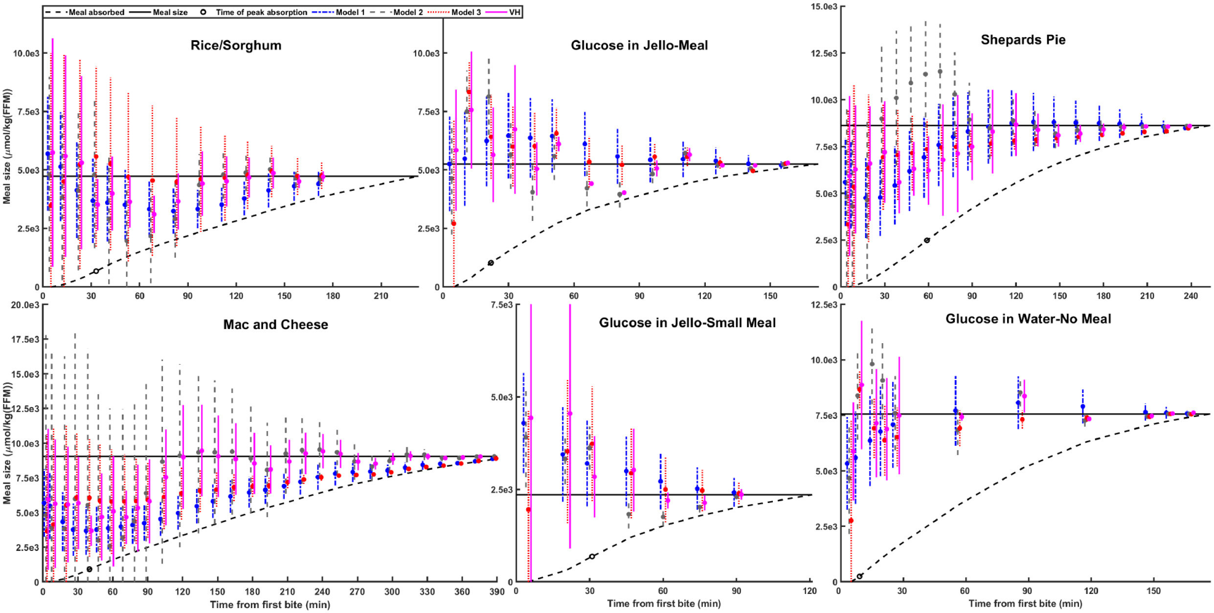
What these methods are missing is the full meal absorption shape. Published data,^31-34 shown in Figure 1, shows cases where meals have similar initial rate of rise (meals 1, 4, 5), but due to different compositions (rice/sorghum, mac and cheese, and glucose in jello), have widely varying meal sizes (area under the curve).

Figure 1.

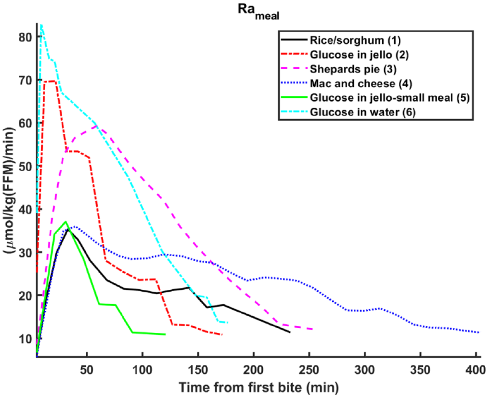
Triple tracer studies of carbohydrate turnover for meals of varying compositions.

Methods relying directly on initial rise to estimate meal size will fail because they assume the meal shape. An assumed meal shape also leads to overconfidence in the meal size estimate, and potential over administration of insulin. Reliable indicators of meal size that reduce uncertainty exist after the rise portion of the meal, but existing methods do not know to wait. Uncertainty of the meal size is accounted for indirectly using conservative insulin dosing strategies,^9,11,30 requirement of persistent excitation,^{8,10,12,13,29} probabilistic modeling methods,¹⁹ or bi-directional control.^27,35

To avoid the issues mentioned above, we propose a meal model that divides meal absorption into two disjoint regions around the peak absorption. Before the peak, there are coarse estimates of meal size, which are fine tuned in post-peak region. The three-model system is composed of a linear rise model pre-peak, and linear drop and exponential decay models post-peak. We use Bayes’ Rule to determine when the peak occurs. We compare the proposed model to other models of increasing complexity.

Background

Many frameworks for detecting and rejecting unannounced meal disturbances have been proposed. The present work is focused on disturbance rejection rather than detection, so only that aspect will be considered in the review of existing work.

Dassau et al.³⁰ proposed an MPC that uses the glucose simulation model developed by Dalla Man et al.^36,37 in addition to a generic meal input from Hovorka et al.³⁷ Lee and Bequette developed an MPC that used a finite impulse response filter to estimate meal size.³⁸ Lee et al. takes a similar approach, compensating for unannounced meals using BG impulses.⁸

Cameron et al. presented a probabilistic multiple model approach to compensate for unannounced meals.¹⁹ Prior probabilities based on the last mealtime are assigned to new models, which assume either a new meal or no meal. Xie and Wang propose a finite impulse response filter that is updated with measurements to estimate meal size.¹⁰

The framework developed by Turksoy et al. uses an Unscented Kalman Filter to estimate the rate of meal carbohydrate appearance.¹¹ When absorption thresholds are reached, a correction bolus is calculated using the current BG and the subject’s body weight in addition to tuning parameters.

Fuzzy qualitative analysis of CGM measurements is used in Samadi et al. to detect meals and estimate size.¹² Singleton fuzzy sets informed by both insulin and CGM are used to increment estimated meal size. Mahmoudi et al. suggested a Rauch-Tung-Striebel smoother to estimate meal size after detection.¹³

In addition to these frameworks, many models describing meal carbohydrate absorption have been developed, ranging from the work of Deutsch³⁹ to the model used in the UVa/Padova simulator.⁴⁰ A review of these models can be found in El Fathi et al.²³

Methods

Data

Data used to evaluate the models are taken from a collection of triple tracer (TT) studies; the TT technique is the gold-standard for measuring the rate of meal carbohydrate appearance.⁴¹ Although not all subjects were people with Type 1 diabetes, it has been shown this has little effect.^34,42,43

Rather than use all available TT data, which consist mostly of standard test meals (egg, bacon, and jello), we chose six distinct meal shapes spanning a range of compositions and sizes. Figure 1 shows the shapes, and Table 1 provides the study details.

Table 1.

The Triple Tracer Datasets, Which Consist of Meals with Varying Compositions and Sizes.

Description	H/T1D/T2D	M	F	Age (year)	CHO (kcal)	Meal (kcal)	C/F/P (%)	Tracer, location
1) 50 g rice/sorghum meal	H	4, 5	4, 3	30.9 ± 7, 34.8 ± 10.5	209	600	35/26/39	Polysaccharide, rice/sorghum
2) 50 g glucose meal	H	4, 5	4, 3	30.9 ± 7, 34.8 ± 10.5	209	600	35/24/41	Glucose, gelatin
3) 121 g HG CHO meal	T1D	4	0	18.1 ± 4	484	615	75/12/13	Glucose, sauce
4) 121 g LG CHO meal	T1D	5	0	20.8 ± 3.3	484	899	54/31/15	Glucose, sauce
5) 35 g Glucose meal	T2D	2	7	58 ± 3	140	220	56/25/19	Glucose, gelatin
6) 75 g Glucose in water	T2D	3	2	56 ± 4	300	300	100/0/0	Glucose, water

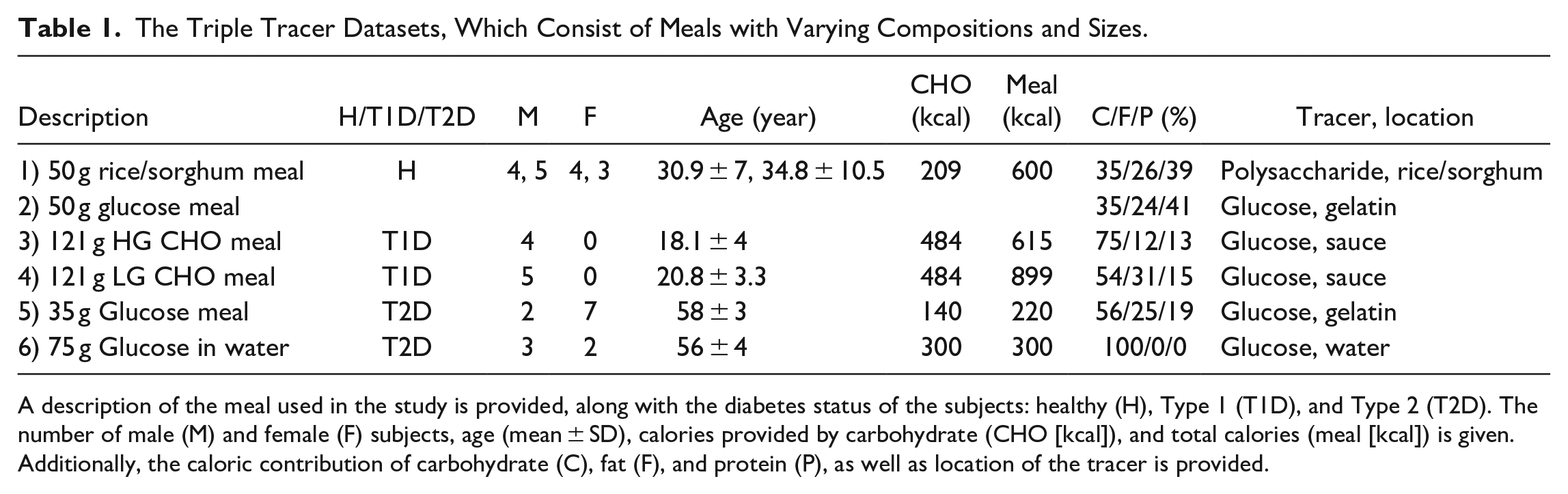
A description of the meal used in the study is provided, along with the diabetes status of the subjects: healthy (H), Type 1 (T1D), and Type 2 (T2D). The number of male (M) and female (F) subjects, age (mean ± SD), calories provided by carbohydrate (CHO [kcal]), and total calories (meal [kcal]) is given. Additionally, the caloric contribution of carbohydrate (C), fat (F), and protein (P), as well as location of the tracer is provided.

TT studies are resource intensive but provide excellent descriptions of postprandial carbohydrate turnover, which are not possible to extract from CGM data because of multiple confounding effects. To study the effect of complex carbohydrates, Basu et al. use the complex carbohydrate itself as the tracer.³¹ Elleri et al. also study the effects of complex carbohydrates but use a glucose tracer, necessitating a different methodology.⁴⁴ Though the method may have drawbacks,³¹ we still include their data. Data from over 50 individuals of differing diabetes conditions are included in the collected dataset.

Model Updating

All proposed models are linear time invariant and can be written as a discrete state space system:

x_{k + 1} = A x_{k} + B u_{k}

y_{k} = C x_{k}

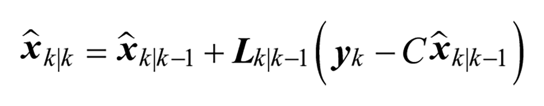
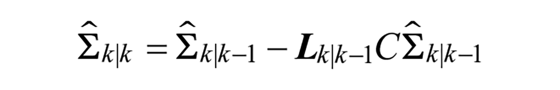
The states and covariance estimates of models are propagated through time and updated from measurements using the Kalman Filter time and measurement update equations:

Time update:

{\hat{x}}_{k + 1} = A {\hat{x}}_{k} + B u_{k} + v

{\hat{Σ}}_{k + 1} = A {\hat{Σ}}_{k} A^{T} + Σ_{v}

${\hat{x}}_{k}$ is the state estimate at time step $k$ , $A$ and $B$ are the state transition and input matrices, respectively. $v ~ ℵ (0, Σ_{v})$ is Gaussian independent and identically distributed (IID) process noise. $u_{k}$ is the system input at time step $k$ . ${\hat{Σ}}_{k}$ is the uncertainty of the estimated state, also referred to as the covariance.

Measurement update:

L_{k | k - 1} = {\hat{Σ}}_{k | k - 1} C^{T} + Σ_{w}

{\hat{x}}_{k | k} = {\hat{x}}_{k | k - 1} + L_{k | k - 1} (y_{k} - C {\hat{x}}_{k | k - 1})

{\hat{Σ}}_{k | k} = {\hat{Σ}}_{k | k - 1} - L_{k | k - 1} C {\hat{Σ}}_{k | k - 1}

$L_{k | k - 1}$ is the Kalman Gain at time step $k$ , given information up to measurement $k - 1$ . ${\hat{Σ}}_{k | k - 1}$ is the state covariance at time step $k$ given information up to measurement $k - 1$ , and $Σ_{w}$ is IID sensor noise. When no measurement is obtained, we assume ${\hat{x}}_{k | k} = {\hat{x}}_{k | k - 1}$ .

Model 1: Second Order Response

The first model proposed is a linear second order response inspired by previously developed two-compartment models.²³ Contents enter the first compartment, $s$ , and empty exponentially in the second, $a$ , where they are absorbed. The model is limited to modulations in amplitude of the meal absorption curve, but not modulations in shape.

{\hat{a}}_{k + 1} = (1 - C_{1}) {\hat{s}}_{k} + C_{2} {\hat{a}}_{k}

{\hat{g}}_{k + 1} = {\hat{g}}_{k} + {\hat{a}}_{k}

{\hat{s}}_{k + 1} = C_{1} {\hat{s}}_{k} + u_{k}

$u_{k}$ is the meal input at time step $k$ . $C_{1}$ and $C_{2}$ are coefficients constrained between 0 and 1 that govern the exponential decay from the two compartments, respectively. $g$ represents the accumulated, or total, meal carbohydrate. The hat operator denotes an estimated state. The full forms of the estimated state vector, covariance matrix, as well as the state transition, input, output, initial covariance, process noise, and sensor noise matrices used in the Kalman Filter equations can be found in the Appendix. Parameter values for all terms are also provided.

Model 2: Augmented Second Order Response

Modulations in shape of the meal absorption curve can be achieved with additional states $r$ and $d$ , the linear rise and drop rate of the curve, respectively.

{\hat{a}}_{k + 1} = (1 - C_{1}) {\hat{s}}_{k} + C_{2} {\hat{a}}_{k} + {\hat{r}}_{k} - {\hat{d}}_{k}

{\hat{g}}_{k + 1} = {\hat{g}}_{k} + {\hat{a}}_{k}

{\hat{s}}_{k + 1} = m a x (0, C_{1} {\hat{s}}_{k} - {\hat{r}}_{k} + u_{k})

{\hat{r}}_{k + 1} = \min ({\hat{r}}_{k}, {\hat{s}}_{k})

{\hat{d}}_{k + 1} = {\hat{d}}_{k}

Model 3: Nonlinear Second Order Response

Model capacity may also be increased with a nonlinear model paired with an Extended Kalman Filter. To accurately describe gastric emptying, a nonlinear model may be necessary.⁴⁵ Towards this end, the coefficient of emptying from the first compartment is estimated as a state, $c$ .

{\hat{a}}_{k + 1} = (1 - {\hat{c}}_{k}) {\hat{s}}_{k} + C_{2} {\hat{a}}_{k}

{\hat{g}}_{k + 1} = {\hat{g}}_{k} + {\hat{a}}_{k}

{\hat{s}}_{k + 1} = {\hat{c}}_{k} {\hat{s}}_{k} + u_{k}

{\hat{c}}_{k + 1} = {\hat{c}}_{k}

Variable Hump Model

The methods previously described represent attempts to increase model capacity but are still fundamentally limited as single models that assume a single shape. To infer both meal size and absorption shape, we propose a multiple model framework of three sub-models.

Linear Rise (1):

{\hat{a}}_{k + 1} = {\hat{a}}_{k} + {\hat{r}}_{k}

{\hat{g}}_{k + 1} = {\hat{g}}_{k} + {\hat{a}}_{k}

{\hat{r}}_{k + 1} = {\hat{r}}_{k} + r_{0} δ

Linear Drop (2):

{\hat{a}}_{k + 1} = {\hat{a}}_{k} - {\hat{d}}_{k} + u_{a, p e a k}

{\hat{g}}_{k + 1} = {\hat{g}}_{k} + {\hat{a}}_{k} + u_{g, p e a k}

{\hat{d}}_{k + 1} = m a x ({\hat{d}}_{k} + {\hat{d}}_{p e a k} δ, 0.01)

Exponential Decay (3):

{\hat{a}}_{k + 1} = {\hat{c}}_{k} {\hat{a}}_{k} + u_{a, p e a k}

{\hat{g}}_{k + 1} = {\hat{g}}_{k} + {\hat{a}}_{k} + u_{g, p e a k}

{\hat{c}}_{k + 1} = m i n ({\hat{c}}_{k} + {\hat{c}}_{p e a k} δ, 0.995)

$u_{a, p e a k}$ and $u_{g, p e a k}$ are the peak absorption and accumulated glucose values, respectively, from the Linear Rise model. $δ$ is the Dirac Delta which initializes the rise, drop, and decay states for the three models, respectively.

The modeling approach, presented in Figure 2, divides the meal absorption curve into two disjoint regions, pre-peak (←) and post-peak (→). Embedded are two switching systems.⁴⁵ The first determines peak time by considering possible models that change from pre-peak to post-peak behavior at a given time. Prior knowledge of peak time is incorporated with Bayes’ Rule. The second, which constitutes post-peak behavior, is a two-model switching system between drop and decay behavior.

Figure 2.

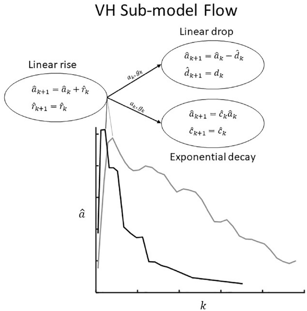
Modeling framework of proposed Variable Hump (VH) Model: After the peak, two models are used to capture different meal shapes.

Pre-peak behavior

The rise sub-model fully governs in the pre-peak region. To detect the peak with Bayes’ rule we reset the drop and decay models every time, $k$ , a measurement is received. The drop and decay sub-model glucose appearance and accumulation states/covariance are initialized from the rise sub-model.

{\hat{z}}_{k}^{i} = {\hat{z}}_{k}^{1} \forall z \in a, g, σ_{a, a}, σ_{g, g}, σ_{a, g}, σ_{g, a} \forall i = 2, 3

The superscript 1 indicates the rise sub-model whereas superscripts 2 and 3 indicate drop and decay sub-models, respectively.

The drop rate $d$ and decay coefficient $c$ are a function of the rate of appearance $a$ , with equations shown in the proceeding section, Peak Absorption Switch. The uncertainty of the drop and decay states are set to initial values:

{\hat{σ}}_{k, (d, d)} = {\hat{σ}}_{0, (d, d)}, {\hat{σ}}_{k, (c, c)} = {\hat{σ}}_{0, (c, c)}

Peak absorption switch

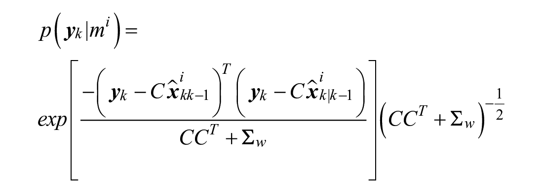
Peak absorption occurs when post-peak behavior is equally or more probable than pre-peak behavior:

p (\to | d_{k}) \geq p (\leftarrow | d_{k})

$p (\leftarrow | d_{k})$ is the probability of pre-peak behavior given the data, while $p (\to | d_{k})$ represents post-peak. If $p (\leftarrow | d_{k}) > p (\to | d_{k})$ , then peak absorption has not occurred. Under this framework, it is possible to revert to pre-peak behavior. To reduce the number of possible models, previous improbable switches are discarded:

p (\to | d_{j}) = 0, \forall j \in {0, \dots, k - 1}

Bayes’ Rule is used to incorporate prior knowledge:

p (\leftarrow | d_{k}) = D p (d_{k} | \leftarrow) p (t_{p e a k} > k)

$p (t_{p e a k} > k)$ is the prior probability of pre-peak behavior at $k$ , which is initialized to unity and decreases linearly to zero over 72 time steps, $p (t_{p e a k} > 0) = 1,$ $p (t_{p e a k} > 72) = 0$ . The constant $D$ normalizes the probability:

D = p (\leftarrow | d_{k}) + p (\to | d_{k})

$p (d_{k} | \leftarrow)$ is the likelihood of observing the data assuming pre-peak behavior. Pre-peak behavior is described by the rise sub-model $(m^{1})$ , and a jump system is assumed:

p (d_{k} | \leftarrow) = p (y_{k} | m^{1})

The innovation’s probability in a Gaussian function of zero mean and standard deviation following sensor noise $Σ_{w}$ is:

\begin{array}{l} p (y_{k} | m^{i}) = \\ e x p [\frac{- {(y_{k} - C {\hat{x}}_{k k - 1}^{i})}^{T} (y_{k} - C {\hat{x}}_{k | k - 1}^{i})}{C C^{T} + Σ_{w}}] {(C C^{T} + Σ_{w})}^{- \frac{1}{2}} \end{array}

$p (\to | d_{k})$ is similar, but post-peak behavior is characterized by an additional two-model switching system, where the drop and decay sub-models have equal prior probability.

p (\to | d_{k}) = D p (d_{k} | \to) p (t_{p e a k} < = k)

p (d_{k} | \to) = \sum_{i = 2}^{3} \frac{1}{2} p (y_{k} | m^{i})

The prior probability of post-peak behavior is the remaining probability from the pre-peak prior:

p (t_{p e a k} < = k) = 1 - p (t_{p e a k} > k)

When behavior switches from pre-peak to post-peak, the drop and decay sub-model’s glucose appearance and accumulation states/covariance are initialized using a probability-weighted combination between all sub-models:

\begin{array}{l} {\hat{z}}_{p e a k} = \sum_{i = 1}^{3} p (m_{i} | d_{p e a k}) {\hat{z}}_{p e a k}^{i} \\ \forall z \in {a, g, σ_{a, a}, σ_{g, g}, σ_{a, g}, σ_{g, a}} \end{array}

To initialize the drop $(d)$ and decay $(c)$ states, we first correlate peak absorption value (found in the above equation) with meal size ( $ρ ~ 0.4$ ).

S = C_{S} {\hat{a}}_{p e a k}

Given the estimated peak absorption value $({\hat{a}}_{p e a k})$ , the drop rate $({\hat{d}}_{p e a k})$ and decay coefficient $({\hat{c}}_{p e a k})$ are calculated from the approximated total meal size $S$ found above.

{\hat{d}}_{p e a k} = \frac{{\hat{a}}_{p e a k}}{2 (C_{S} {\hat{a}}_{p e a k} - {\hat{g}}_{p e a k})}

{\hat{c}}_{p e a k} = 1 - \frac{{\hat{a}}_{p e a k}}{C_{S} {\hat{a}}_{p e a k} - {\hat{g}}_{p e a k}}

A higher peak absorption value $({\hat{a}}_{p e a k})$ yields a steeper drop/decay (higher $\hat{d}$ , lower $\hat{c}$ ), and vice-versa. After initializing the drop and decay states, we set their respective uncertainties $({\hat{σ}}_{k, (d, d)}, {\hat{σ}}_{k, (c, c)})$ to initial values $({\hat{σ}}_{0, (d, d)}, {\hat{σ}}_{0, (c, c)})$ as before.

The final item we consider at the peak is uncertainty. Following the assumptions that (1) meals with an absorption peak of zero (ie, meal size of zero) have no uncertainty, (2) uncertainty increases with predicted meal size, and (3) uncertainty increases with larger peak absorption uncertainty, we scale the uncertainty matrices. The scale, $C_{Σ}$ , is found using the estimated normal distribution of peak absorption $ℵ ({\hat{a}}_{p e a k}, \sqrt{{\hat{σ}}_{p e a k, (a, a)}})$ :

C_{Σ} = \frac{f}{10} \sum_{j = 5 %}^{95 %} {(\frac{x_{j}}{μ_{p e a k}})}^{2}

x_j represents sample points from the estimated distribution of peak absorption $ℵ ({\hat{a}}_{p e a k}, \sqrt{{\hat{σ}}_{p e a k, (a, a)}})$ , evaluated at evenly spaced probability values, while $µ_{p e a k}$ is the mean value of peak absorption from the TT dataset. $f$ serves as a tuning parameter that adjusts the magnitude of meal size uncertainty.

Post-peak behavior

Post-peak behavior is characterized by a two-model switching system between the drop and decay sub-models. Bayes’ Rule is modified to consider all measurements since the peak:

p (m_{i} | d_{k}) = D p (d_{k} | m_{i})

p (d_{k} | m_{i}) = \prod_{j = p e a k}^{n o w} p (y_{j} | m_{i})

D = \frac{1}{\sum_{j = 2}^{3} p (y_{k} | m_{i}) p (m_{i})}

Note that the prior probability term $p (m_{k}^{i})$ has been omitted since both the drop and decay sub-models have equal prior probabilities.

Prediction

To predict, the VH model states and covariance matrices are propagated into the future without measurement updates via the KF time update equations. Final predictions are a probability-weighted combination of the sub-models. This requires a prediction of the weights assigned to the sub-models.

To predict from the pre-peak region, the peak absorption time ( $t_{p e a k})$ and magnitude ( $a_{p e a k})$ are predicted. We start by constructing triangular probability density functions (PDF) to approximate $t_{p e a k}$ and $a_{p e a k}$ data from the TT dataset. The two PDFs, denoted by $f (t_{p e a k})$ and $f (a_{p e a k})$ respectively, are conditioned on the current time step $k$ or absorption value $a_{k}$ :

f (t_{p e a k} | t_{p e a k} \geq k) = \frac{f (t_{p e a k} \geq k}}{1 - F (t_{p e a k} = k)}

f (a_{p e a k} | a_{p e a k} \geq a_{k}) = \frac{f (a_{p e a k} \geq a_{k}}}{1 - F (a_{p e a k} = a_{k})}

$F (t_{p e a k})$ is the cumulative distribution function of peak absorption time, and $F (t_{p e a k} = k)$ represents the probability that the peak absorption time is less than or equal to time $k$ . $f (t_{p e a k} \geq k)$ is a PDF for the subset of times that are greater than or equal to the current time $k$ . Similar logic is applied for $a_{p e a k}$ .

To predict peak absorption time and magnitude, let ${\bar{t}}_{p e a k}$ represent the set of possible future peak times, and ${\bar{a}}_{p e a k}$ represent the set of future peak values according to the currently estimated rise rate ${\hat{r}}_{k}$ :

{\bar{t}}_{p e a k} = {t_{k}, t_{k + 1}, \dots, t_{k + i}}

{\bar{a}}_{p e a k} = {a_{k}, a_{k + 1}, \dots, a_{k + i}}

The peak occurs at the time step $k + i$ that satisfies:

(1 - F (t_{k + i})) (1 - F (a_{k + i})) < {(0.5)}^{2}

Letting $w_{t_{1} : t_{2}}^{j}$ denote the weight applied to model $j$ from time steps $t_{1}$ to $t_{2}$ , we assign the following weights:

w_{k : k + i}^{1} = 1, | w_{k + i : k + p}^{1} = 0

w_{k : k + i}^{j} = 0, | w_{k + i : k + p}^{j} = 0.5, | \forall j \in {2, 3}

$k : k + i$ spans the pre-peak region, while $k + i : k + p$ spans the post-peak region. The prediction horizon $p$ extends out to the length of TT data for the given curve. ${\hat{d}}_{p e a k}$ , ${\hat{c}}_{p e a k}$ , and $C_{Σ}$ are calculated before as in Peak Absorption Switch.

Calculating the predicted weights is much simpler when predicting from the post-peak region:

w_{k : k + p}^{1} = 0

w_{k : k + p}^{j} = p (m_{j} | d_{k}), | \forall j \in {2, 3}

Model invalidation

When infeasible states are estimated, we choose to constrain the model in both state and covariance. If the rise rate $r$ in the rise sub-model becomes negative:

A^{1} = [\begin{matrix} 1 & 0 & 0 \\ 1 & 1 & 0 \\ 0 & 0 & 0 \end{matrix}]

This has the effect of holding absorption constant. If the estimated glucose absorption of the drop sub-model becomes negative, ${\hat{a}}^{j = 2} < 0$ , or a threshold is passed for the decay sub-model, ${\hat{a}}^{j = 3} < h_{c}$ , then:

A^{j} = [\begin{matrix} 0 & 0 & 0 \\ 0 & 1 & 0 \\ 0 & 0 & 0 \end{matrix}], for model j

Model Evaluation

Capability of model fit to data is determined by optimization of model parameters ( $C_{n}$ ) and initial model states ( ${\hat{x}}_{0}$ ) using Matlab’s^™ fmincon routine. For the VH Model, time of peak was considered along with rise, drop, and decay states ( $r, d, c$ respectively), with post-peak behavior influenced by both drop and decay sub-models evenly.

Prediction accuracy is evaluated by performing Kalman Filtered predictions at every measurement update. Starting model state was initialized to the mean of all optimal initial states found above, while initial model uncertainty was initialized to the variance. Values for sensor $(Σ_{w})$ and additive process noise $(Σ_{v})$ were optimized for all models.

The ability of each model to estimate the time of peak absorption was considered. To evaluate how well each model predicts its accuracy, the actual percentage of readings within symmetric confidence bounds of a given theoretical percentage were tallied. Finally, we examine a simple implementation of the models.

Results

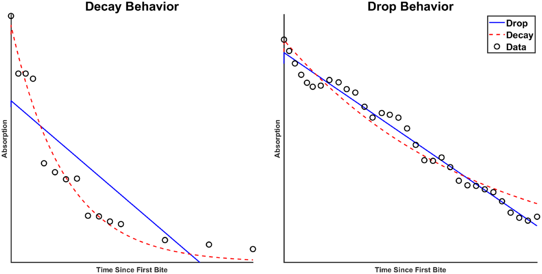
Within the VH Model, adaptability to the meal shape is aided by using two sub-models post-peak. Behavior is better described by the decay sub-model in some cases and by the drop sub-model in others. In the left panel of Figure 3, the decay (red) provides a better fit to the data than the linear drop (RMSE: 235 vs 2051 $μ m o l / k g (F F M) / m i n$ , respectively). In the right panel, the opposite is true (RMSE: 129 vs 48 $μ m o l / k g (F F M) / m i n$ , respectively).

Figure 3.

Some curves are better described by a decay behavior (left), whereas others a drop behavior (right). The left panel shows the least-squares fits to Meal 2, while the right panel shows fits to Meal 4. Absorption has units of µmol/kg (FFM)/min. FFM: fat free mass.

Among all models, Model 1, which assumes a single shape, is the least capable of fitting the data per Table 2. Models 2 and 3, which allow modulations in shape, provide better fit. The multiple-model VH framework is the most capable of fitting the data.

Table 2.

Fit, Prediction Accuracy, and Run Time of the Evaluated Models on the Triple Tracer Dataset.

Model	Fit RMSE (μmol/KG[FFM]/min)	Prediction RMSE (μmol/KG[FFM])	Run time (s)
Model 1	51	1726	0.0012
Model 2	18	1691	0.0016
Model 3	28	1544	0.0033
VH Model	14	1358	0.0389

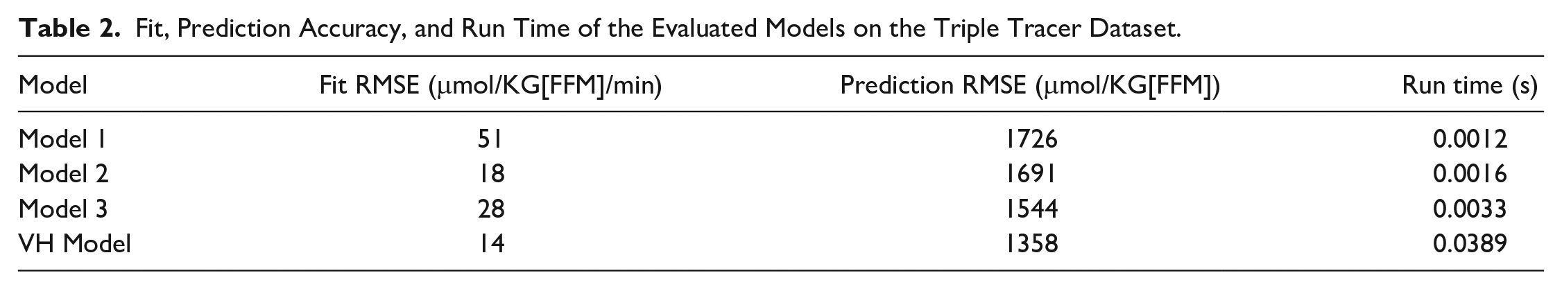
Prediction accuracy follows a similar trend as model fit, but Model 3 provides superior predictions compared to Model 2. The VH model most accurately predicts total meal size, showing a 21% improvement over Model 1 and an 11% improvement over Model 3. The trend of predicted meal size across all meals and models is shown in Figure 4. Specifically, the predicted meal size ( $mean \pm SD$ ) is shown for predictions made at each measurement update after meal consumption, along with the actual meal size and actual accumulated glucose over time. Generally, predictions from all models become more accurate and decrease in uncertainty when moving further into the meal. The VH Model adapts better to quick and slow meals (Meals 4 and 5, respectively), while other models either fail to adapt or overestimate (Meals 4 and 3, respectively).

Figure 4.

Evolution of predicted meal size $(μ \pm 1 σ)$ over time into the meal. Errors are single dots and symmetric confidence bounds are lines (dash-dotted: Model 1, dash: Model 2, dotted: Model 3, solid: VH Model). The VH Model adapts to the meal while other models either fail to (Meal 4) or overestimate (Meal 3). VH: Variable Hump.

Figure 5 shows residuals of the model-estimated peak time from the true peak time (vertical black line). A constant peak time (depicted by digits 1-6) equal to the mean of the dataset peak times (32 minutes) is included for comparison. Arrows represent the adaption from the constant peak time to the VH estimated peak time. The VH model most accurately estimates the true RA peak time, see Table 3. Additionally, the empirical cumulative distribution functions of the actual peak times along with model-estimated peak times is presented in the Appendix (Figure S1).

Figure 5.

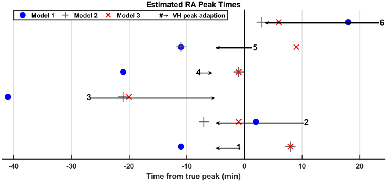
Residuals of estimated model-absorption peak time from time of true absorption peak (blue dot: Model 1, gray +: Model 2, red x: Model 3, black arrowhead: VH Model, #: Assumed constant peak time of 32 minutes). An arrow connects the assumed constant peak time (32 minutes) to the VH Model estimated peak time. VH: Variable Hump.

Table 3.

Mean Absolute Error (Minutes) of the Estimated Peak Absorption for All Models.

Model	Estimated peak time MAE (min)
Model 1	21
Model 2	11
Model 3	10
VH Model	5
Peak at 32 min	15

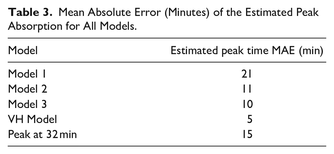
Figure 6 shows how well each model predicts its accuracy. Specifically, it shows agreement between the theoretical confidence interval of predicted meal size and the actual coverage. Intervals of theoretical confidence spanning 1%-99% are generated using:

[\begin{array}{l} C {\hat{x}}_{k + p k} - α (C {\hat{Σ}}_{k + p k} C^{T} + Σ_{W}), \\ C {\hat{x}}_{k + p k} + α (C {\hat{Σ}}_{k + p k} C^{T} + Σ_{W}) \end{array}]

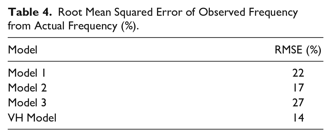
A model with perfect predictions of uncertainty would follow the 1:1 line in Figure 6. The VH Model provides the closest agreement between the theoretical and actual coverage, see Table 4.

Figure 6.

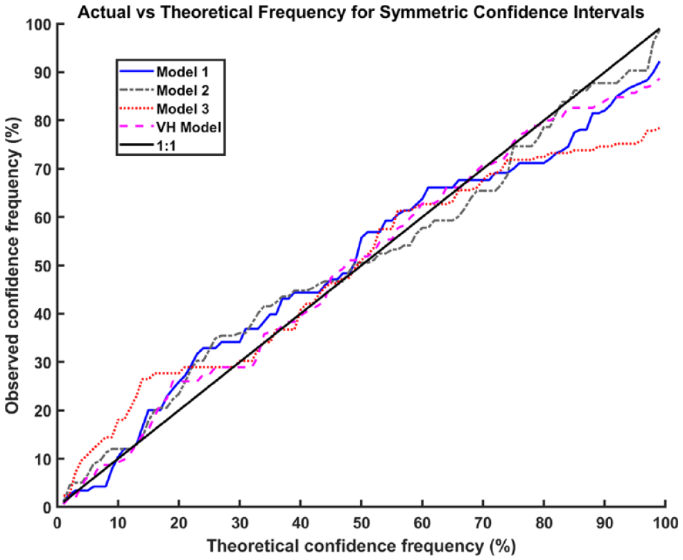
Agreement between symmetric confidence intervals of a theoretical width with the actual percentage of readings within the interval.

Table 4.

Root Mean Squared Error of Observed Frequency from Actual Frequency (%).

Model	RMSE (%)
Model 1	22
Model 2	17
Model 3	27
VH Model	14

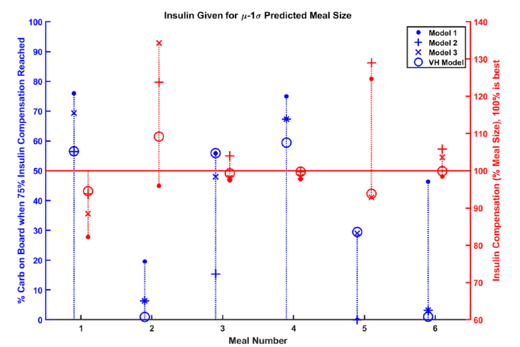
A simple implementation is considered in Figure 7. Since underestimation is preferred, we compensate with insulin assuming a meal size equal to the lower bound of predicted meal size $(m e a n - 1 S D)$ . The left axis represents the speed at which a model compensates for the meal, and quicker responses are desired. The right axis represents the maximum compensation from a model, and compensation close to 100% is desired.

Figure 7.

Since underestimation of meal sizes is preferred to overestimation, one may choose to deliver insulin assuming a meal size determined from the lower bound of predicted meal size (µ-1σ). Compensation for 75% of the meal is shown on the left axis and as blue data. The total insulin compensation is shown on the right axis and as red data.

In four out of six meals, the controller governed by the VH Model is the quickest to compensate for 75% of the meal. A controller that over-compensates is considerably handicapped because of the safety implications of hypoglycemia. In at least one meal, the controllers for Models 1-3 overcompensate by at least 25%, while the maximum overcompensation for the VH Model controller is 9%.

Increases in model capacity should be weighed against added computational burden since model predictions must be made online in an AP. The run-time required to make a prediction was: 0.0011 s, 0.0014 s, 0.0030 s, and 0.035 s for Models 1, 2, 3, and VH, respectively.

Discussion

The drawbacks of assuming a single meal shape are shown with Model 1, which yielded prediction performance comparable to the VH model on meals with simple carbohydrates (total MSE for Meals 2, 5, and 6: 8.00e5 vs 8.01e5, respectively) but not slow meals with complex carbohydrates (total MSE for Meals 1, 3, and 4: 5.16e6 vs 2.92e6, respectively). While Model 3 adapts to complex carbohydrate meals (MSE: 3.23e6), prediction accuracy is degraded on the simple carbohydrate meals (MSE: 1.54e6). Model adaptability clearly matters, but single models (Models 1-3) present a trade-off between prediction accuracy and adaptation.

Research suggests that gastroparesis affects 40% of individuals with Type 1 Diabetes.⁴⁶ This logically increases digestive variability, leading to varied postprandial BG responses. A model that can describe and adapt to a wide array of meal types, such as the VH Model, would be preferred in these cases.

Variability in the time of peak absorption is not captured when a fixed peak time is assumed. The VH model, which explicitly considers the peak, exhibits the largest degree of adaptation, as shown in Figure 5 and Table 3. The rounded peak in Meal 3 (Shepard Pie) appears as an outlier compared to the sharp peak transition characteristic of the other meals. The late peak combined with inter-individual variability of digestion speed might have exacerbated the difference in glucose absorption profiles, leading to a rounded peak after averaging. The VH model expects a sharp transition and initially estimates a peak absorption time at 34 minutes after the first bite of the meal. However, the VH Model has the capability to revert to pre-peak rise behavior and estimates a refined peak absorption time at 54 minutes while all other models estimate a peak time much earlier than what actually occurs (Figure 5).

Erroneous control decisions present severe consequences in BG control, particularly hypoglycemia. A model that correctly predicts its accuracy, such as the VH Model, is desired because a substantial amount of insulin is delivered following meal consumption.

Insulin needs to be fast and accurate to attenuate the effects of meals. By considering the possibility of different meal shapes while remaining uncertain until appropriate, the VH model excels at providing fast and accurate insulin in the potential implementation (Figure 7).

Conclusion

In conclusion, we introduced a model with increased capacity to describe varying meal shapes. The model infers both size and shape of the meal by adapting around the peak. To address the inherent uncertainty before the peak, the multiple model framework considers two disjoint regions that consist of coarse and fine-grain predictions of meal size, respectively. Using gold-standard data, we show improvement over simpler models in terms of (1) fit capacity, (2) prediction accuracy, (3) peak time estimation, (4) prediction of accuracy, and (5) a hypothetical control scenario. The small dataset limits this work to a proof of concept study, but a retrospective analysis of prediction accuracy on real data may reveal more benefits of this new approach.

Supplemental Material

sj-pdf-1-dst-10.1177_1932296821990111 – Supplemental material for A New Meal Absorption Model for Artificial Pancreas Systems

Supplemental material, sj-pdf-1-dst-10.1177_1932296821990111 for A New Meal Absorption Model for Artificial Pancreas Systems by Travis Diamond, Faye Cameron and B. Wayne Bequette in Journal of Diabetes Science and Technology

Footnotes

Acknowledgements

The authors would like to acknowledge Pranesh Navarathna for his helpful comments during the drafting process.

Abbreviations

AP, Artificial Pancreas; BG, Blood Glucose; CGM, Continuous Glucose Monitor; CDF, Cumulative Distribution Function; EKF, Extended Kalman Filter; FFM, Fat Free Mass; IID, Independent and Identically Distributed; MSE, Mean Square Error; MPC, Model Predictive Control; PID, Proportional-Integral-Derivative; PDF, Probability Density Function; RMSE, Root Mean Square Error; TT, Triple Tracer; VH, Variable Hump.

Declaration of Conflicting Interests

The author(s) declared no potential conflicts of interest with respect to the research, authorship, and/or publication of this article.

Funding

The author(s) disclosed receipt of the following financial support for the research, authorship, and/or publication of this article: This work was supported by NIH grant 1R01DK102188, and JDRF 1-SRA-2019-817-S-B.

ORCID iDs

Travis Diamond

B. Wayne Bequette

Supplemental Material

Supplemental material for this article is available online.

References

Bekiari

Kitsios

Thabit

, et al. Artificial pancreas treatment for outpatients with type 1 diabetes: systematic review and meta-analysis. BMJ. 2018;361:k1310. doi:10.1136/bmj.k1310

Crabtree

TSJ

McLay

Wilmot

. DIY artificial pancreas systems: here to stay? Pract Diabetes. 2019;36:63-68.

Kowalski

Pathway to artificial pancreas systems revisited: moving downstream. Diabetes Care. 2015;38(6):1036-1043.

Bequette

BW.

Challenges and recent progress in the development of a closed-loop artificial pancreas. Annu Rev Control. 2012;36(2):255-266.

Bequette

BW.

Algorithms for a closed-loop artificial pancreas: the case for model predictive control. J Diabetes Sci Technol. 2013;7(6):1632-1643.

Muske

Badgwell

TA.

Disturbance modeling for offset-free linear model predictive control. J Process Control. 2002;12(5):617-632.

Dassau

Bequette

Buckingham

, et al. Detection of a meal using continuous glucose monitoring. Diabetes Care. 2008;31(2):295-300.

Lee

Buckingham

Wilson

, et al. A closed-loop artificial pancreas using model predictive control and a sliding meal size estimator. J Diabetes Sci Technol. 2009;3(5):1082-1090.

Harvey

Dassau

Zisser

, et al. Design of the glucose rate increase detector: a meal detection module for the health monitoring system. J Diabetes Sci Technol. 2014;8(2):307-320.

10.

Xie

Wang

A variable state dimension approach to meal detection and meal size estimation: in silico evaluation through basal-bolus insulin therapy for type 1 diabetes. IEEE Trans Biomed Eng. 2017;64(6):1249-1260.

11.

Turksoy

Samadi

Feng

, et al. Meal detection in patients with type 1 diabetes: a new module for the multivariable adaptive artificial pancreas control system. IEEE J Biomed Health Inform. 2016;20(1):47-54.

12.

Samadi

Turksoy

Hajizadeh

, et al. Meal detection and carbohydrate estimation using continuous glucose sensor data. IEEE J Biomed Health Inform. 2017;21(3):619-627.

13.

Mahmoudi

Cameron

Poulsen

, et al. Sensor-based detection and estimation of meal carbohydrates for people with diabetes. Biomed Signal Process Control. 2019;48:12-25.

14.

Ramkissoon

Herrero

Bondia

, et al. Unannounced meals in the artificial pancreas: detection using continuous glucose monitoring. Sensors (Switzerland). 2018;18(3):1-18.

15.

Kölle

Biester

Christiansen

, et al. Pattern recognition reveals characteristic postprandial glucose changes: non-individualized meal detection in diabetes mellitus type 1. IEEE J Biomed Health Inform. 2020;24(2):594-602.

16.

Weimer

Chen

Peleckis

, et al. Physiology-invariant meal detection for type 1 diabetes. Diabetes Technol Ther. 2016;18(10):616-624.

17.

Chen

Paoletti

Smolka

Lin

Committed Moving Horizon Estimation for Meal Detection and Estimation in Type 1 Diabetes. Presentation at: Proceedings of the American Control Conference; July 10-12, 2019; Philadelphia, PA, pp. 4765-4772.

18.

Zheng

Kleinberg

Automated meal detection from continuous glucose monitor data through simulation and explanation. J Am Med Inform Assoc. 2019;26(12):1592-1599.

19.

Cameron

Niemeyer

Bequette

BW.

Extended multiple model prediction with application to blood glucose regulation. J Process Control. 2012;22(8):1422-1432.

20.

Holst

Gribble

Horowitz

, et al. Roles of the gut in glucose homeostasis. Diabetes Care. 2016;39(6):884-892.

21.

Brownlee

Gill

Wilcox

, et al. Starch digestion in the upper gastrointestinal tract of humans. Starch. 2017;70(9-10):1700111.

22.

Okabe

Terashima

Sakamoto

A comparison of gastric emptying of soluble solid meals and clear fluids matched for volume and energy content: a pilot crossover study. Anaesthesia. 2017;72(11):1344-1350.

23.

Fathi

Gingras

Boulet

The artificial pancreas and meal control. IEEE Control Systems. 2018;38(1):30-46.

24.

Slattery

Amiel

Choudhary

Optimal prandial timing of bolus insulin in diabetes management: a review. Diabet Med. 2018;35(3):306-316.

25.

Jones

Quarry

Caldwell-Mcmillan

, et al. Optimal insulin pump dosing and postprandial glycemia following a pizza meal using the continuous glucose monitoring system. Diabetes Technol Ther. 2005;7(2):233-240.

26.

Paterson

Bell

O’Connell

, et al. The role of dietary protein and fat in glycaemic control in type 1 diabetes: implications for intensive diabetes management. Curr Diab Rep. 2015; 15(9):1-9.

27.

van Bon

Jonker

Koebrugge

, et al. Feasibility of a bihormonal closed-loop system to control postexercise and postprandial glucose excursions. J Diabetes Sci Technol. 2012;6(5):1114-1122.

28.

Samadi

Rashid

Turksoy

, et al. Automatic detection and estimation of unannounced meals for multivariable artificial pancreas system. Diabetes Technol Ther. 2018;20(3):235-246.

29.

Hajizadeh

Rashid

Sevil

, et al. Adaptive model predictive control for nonlinearity in biomedical applications. IFAC-PapersOnLine. 2018;51(20):368-373.

30.

Dassau

Herrero

Zisser

, et al. Implications of meal library & meal detection to glycemic control of type 1 diabetes mellitus through MPC control. IFAC Proc Volumes. 2008;41(2):4228-4233.

31.

Basu

Schiavon

Petterson

, et al. A novel natural tracer method to measure complex carbohydrate metabolism. Am J Physiol Endocrinol Metab. 2019;317(3):E483-E493.

32.

Elleri

Allen

Harris

, et al. Absorption patterns of meals containing complex carbohydrates in type 1 diabetes. Diabetologia. 2013;56(5):1108-1117.

33.

Sathananthan

Shah

Edens

, et al. Six and 12 weeks of caloric restriction increases β cell function and lowers fasting and postprandial glucose concentrations in people with type 2 diabetes. J Nutr. 2015;145(9):2046-2051.

34.

Xia

Zhang

Zhu

Trace glucose fluxes in individuals with prediabetes using stable isotopes. Chin Med J (Engl). 2014;127(9):1726-1731.

35.

El-Khatib

Russell

Nathan

, et al. Bi-hormonal closed-loop glucose control for type 1 diabetes. Sci Transl Med. 2010;2(27):1-17.

36.

Dalla Man

Rizza

Cobelli

Meal simulation model of the glucose-insulin system. IEEE Trans Biomed Eng. 2007;54(10):1740-1749.

37.

Hovorka

Canonico

Chassin

, et al. Nonlinear model predictive control of glucose concentration in subjects with type 1 diabetes. Physiol Meas. 2004;25(4):905-920.

38.

Lee

Bequette

BW.

A closed-loop artificial pancreas based on model predictive control: human-friendly identification and automatic meal disturbance rejection. Biomed Signal Process Control. 2009;4(4):347-354.

39.

Lehmann

Deutsch

A physiological model of glucose-insulin interaction in type 1 diabetes mellitus. J Biomed Eng.1992;14(3):235-242.

40.

Dalla Man

Camilleri

Cobelli

. A system model of oral glucose absorption: validation on gold standard data. IEEE Trans Biomed Eng. 2006;53(12 Pt 1):2472-2478.

41.

Basu

di Camillo

Toffolo

, et al. Use of a novel triple-tracer approach to assess postprandial glucose metabolism. Am J Physiol Endocrinol Metab. 2003;284(1):E55-E69.

42.

Basu

Dalla

Basu

, et al. Effects of type 2 diabetes on insulin secretion, insulin action, glucose effectiveness, and postprandial glucose metabolism. Diabetes Care. 2009;32(5):866-872.

43.

Bock

Man

Campioni

, et al. Pathogenesis of pre-diabetes: mechanisms of fasting and postprandial hyperglycemia in people with impaired fasting glucose and/or impaired glucose tolerance. Diabetes. 2006;55(12):3536-3549.

44.

Hovorka

Kumareswaran

Harris

, et al. Overnight closed loop insulin delivery (artificial pancreas) in adults with type 1 diabetes: crossover randomised controlled studies. BMJ. 2011;342:d1855.

45.

Mazor

Averbuch

Bar-Shalom

, et al. Interacting multiple model methods in target tracking: a survey. IEEE T Aero Elec Sys. 1998;34(1):103-123.

46.

Lyrenäs

Olsson

EHK

Arvidsson

, et al. Prevalence and determinants of solid and liquid gastric emptying in unstable type I diabetes: relationship to postprandial blood glucose concentrations. Diabetes Care. 1997;20(3):413-418.

Supplementary Material

Please find the following supplemental material available below.

For Open Access articles published under a Creative Commons License, all supplemental material carries the same license as the article it is associated with.

For non-Open Access articles published, all supplemental material carries a non-exclusive license, and permission requests for re-use of supplemental material or any part of supplemental material shall be sent directly to the copyright owner as specified in the copyright notice associated with the article.

0.00 MB

0.13 MB