
Abstract
Background:
Many glycemic variability (GV) indices exist in the literature. In previous works, we demonstrated that a set of GV indices, extracted from continuous glucose monitoring (CGM) data, can distinguish between stages of diabetes progression. We showed that 25 indices driving a logistic regression classifier can differentiate between healthy and nonhealthy individuals; whereas 37 GV indices and four individual parameters, feeding a polynomial-kernel support vector machine (SVM), can further distinguish between impaired glucose tolerance (IGT) and type 2 diabetes (T2D). The latter approach has some limitations to interpretability (complex model, extensive index pool). In this article, we try to obtain the same performance with a simpler classifier and a parsimonious subset of indices.
Methods:
We analyzed the data of 62 subjects with IGT or T2D. We selected 17 interpretable GV indices and four parameters (age, sex, BMI, waist circumference). We trained a SVM on the data of a baseline visit and tested it on the follow-up visit, comparing the results with the state-of-art methods.
Results:
The linear SVM fed by a reduced subset of 17 GV indices and four basic parameters achieved 82.3% accuracy, only marginally worse than the reference 87.1% (41-features polynomial-kernel SVM). Cross-validation accuracies were comparable (69.6% vs 72.5%).
Conclusion:
The proposed SVM fed by 17 GV indices and four parameters can differentiate between IGT and T2D. Using a simpler model and a parsimonious set of indices caused only a slight accuracy deterioration, with significant advantages in terms of interpretability.
Keywords
The concept of glycemic variability (GV) encompasses the description of the dynamic properties of blood glucose (BG) concentration. With the advent of continuous glucose monitoring (CGM), the quantification of GV has become an established theme in the literature.1,2 For this purpose, a plethora of GV indices has been proposed, each emphasizing different characteristics of BG traces and showing relationships with an increased frequency and severity of complications and unfavorable outcomes.3-5 Recent studies have also investigated whether suitable sets of CGM-extracted GV indices can reflect different stages of diabetes progression, as detected by HbA1c, OGTT, or fasting glucose measurements. Particularly in Acciaroli et al, 6 the authors compute 25 literature GV indices from CGM traces, feed them to a cascade of logistic regression classifiers, and successfully distinguish (cross-validation accuracy of 91.4%) healthy subjects from those with either impaired glucose tolerance (IGT) or type 2 diabetes (T2D). In Longato et al, 7 the subsequent distinction between IGT and T2D has since been addressed by considering more GV indices, complementing them with basic individual parameters, and using a more complex model (accuracy of 87.1%). This satisfactory result, however, came at the cost of ease of interpretation, as it relied on a complex model—a support vector machine (SVM) with a polynomial kernel—that, by design, sacrifices a clear input-output relationship to boost performance.8,9 Furthermore, due to the lack of a definite consensus within the community1,10-12 on the best subset of GV indices for this task, the utilized feature set was extensive and prone to redundancy.
In the present article, we address these limitations and overcome them by working, in parallel, on two fronts: we reduce the number of GV indices by privileging those deemed of most immediate significance, and we forego the application of the kernel trick to our SVM. We demonstrate that these simplifications lead to comparable performance (82.3% accuracy) relative to the complex model presented in Longato et al, 7 arguably with a significant gain in terms of usability and interpretability.
Methods
Database
The present work considers the 62 subjects (31 male, 31 female; aged 44 to 75) affected by IGT or T2D previously analyzed in Longato et al. 7 These subjects participated in the Botnia Prospective Study and the Botnia PPP Study (approved by the ethics committee of Helsinki University Hospital) and were monitored during the EU FP7 Mosaic Project. 13 They were equipped with iPro CGM systems (Medtronic MiniMed, Inc, Northridge, CA, USA), which measured their blood glucose levels at a frequency of one sample every five minutes for two 6-day intervals, spaced one year apart (first semesters of 2014 and 2015; see Figure 1 for an example). During these annual visits, each subject also had his or her BMI and waist circumference recorded and was diagnosed with either IGT or T2D via an oral glucose tolerance test. 14 At the baseline, the two conditions respectively affected 36 and 26 subjects. After a year, two patients reverted from T2D to IGT, while one IGT patient developed full-fledged T2D. In total, 37 and 25 subjects were affected by IGT and T2D at the time of their second visit.
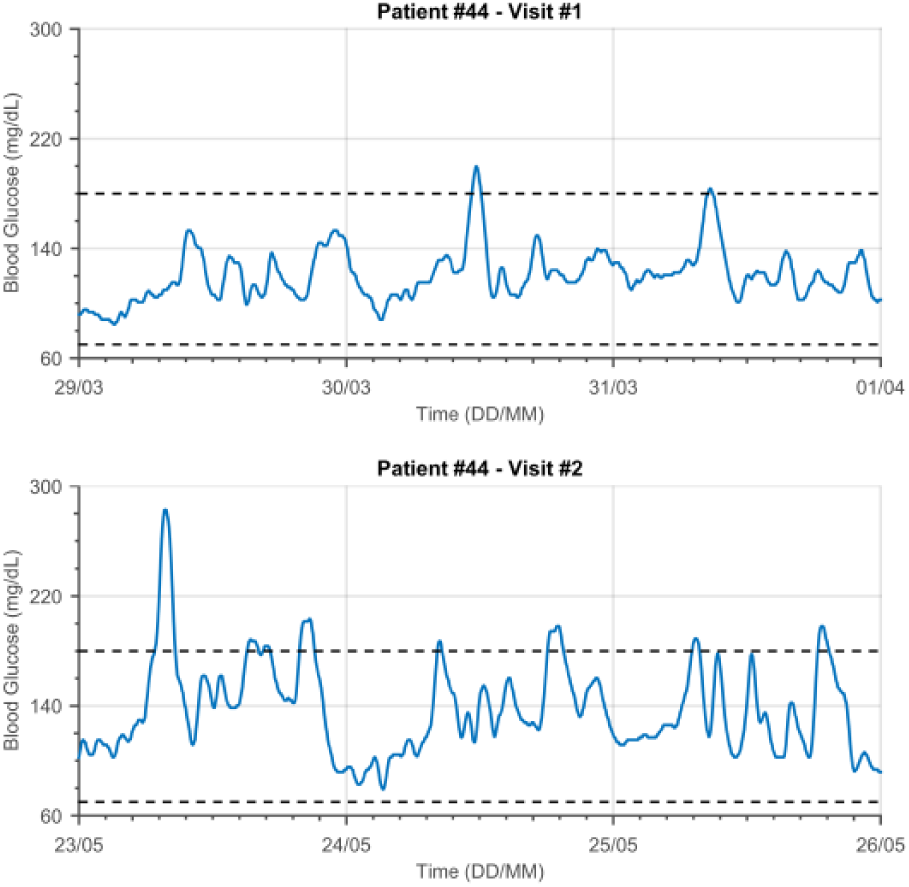
Exemplificative raw data. The top and bottom panel show the CGM traces of a 70-year-old woman, affected by T2D, relative to her first and second visits (March 2014, May 2015).
Glycemic Variability Indices
Initially, we extracted from the raw CGM signals the same set of 37 GV indices used in Longato et al. 7 Then, we selected a subset of 17 of them on the basis of the following two considerations: (1) the selected indices should have an intuitive interpretation, and (2) they should not be overly redundant, but, at the same time, their combination should describe several different aspects of CGM traces.
We used six indices to capture the general statistical properties of the CGM signal: mean and median glucose, standard deviation (SD), coefficient of variation (CV), range, and interquartile range (IQR).2,15 A second subset of two metrics (%BGwithin and %BGbelow)15,16 quantified the proportion of time spent in the euglycemic and hypoglycemic states. We summarized the amplitudes and rates of occurrence of peak-nadir excursions with the MAGE+, MAGE-,17,18 and excursion frequency (EF)19-21 indices. Finally, among the metrics that rely on empirical transformations of the glycemic scale to rescale and properly compare hypo- and hyperglycemia with the euglycemic state, we selected GRADEhypo, GRADEhyper, 22 Hypo Index, Hyper Index, 23 LBGI, and HBGI.24,25
Remark
Of the 37 GV indices used in Longato et al, 7 we excluded SDw, SDd, 26 CONGA, MODD, 27 ADRR,24,25 and Hu’s moment invariants 28 because their mathematical formulations detract from the immediacy of their interpretations and, at the same time, their assessment can, in some cases, prove challenging. To obtain a more parsimonious subset, we also excluded those indices that we expected to carry redundant information with respect to the selected ones: J-index (nonlinear combination of mean and SD), 29 %BGabove (it, %BGwithin, and %BGbelow sum to 100). MAGE (average of MAGE+ and MAGE-), GRADE and GRADEeu (GRADEhypo and GRADEhyper carry similar or complementary information), M-value (extremely similar to GRADE), 30 IGC (sum of Hypo Index and Hyper Index), and BGRI (sum of LBGI and HBGI).
As in Longato et al, 7 we used four “basic” individual parameters—age, sex, BMI, and waist circumference—as additional inputs of the classifier.
Classification Strategy
We split the dataset between a training and a test sets, following the natural subdivision in two annual visits of the data: the 62 data points acquired during the first visit were used in the training phase, and the remaining 62 for performance assessment. This is consistent with the observation reported in Longato et al 7 that, in practice, it would be unrealistic for our method to be usable only after a year-long clinical trial.
As a preprocessing step, we standardized the data, to make each feature have zero mean and unit variance. We estimated the means and standard deviations needed for this transformation on the training set and used them to normalize both it and the test data. In the following, especially regarding cross-validation, we will not explicitly mention normalization; it is implied that we compute the appropriate means and standard deviations to prevent information leak between portions of the data that should remain independent.
To distinguish between IGT and T2D based on the reduced subset of indices (including the four basic parameters) discussed in the Glycemic Variability Indices section, we trained a soft-margins SVM.8,9 SVMs are powerful linear classifiers that attempt to find the best hyperplane to separate the members of two classes (in this case, IGT and T2D). In this respect, they are comparable to the logistic regression used in Acciaroli et al; 6 however, the two techniques differ in their definition of the “best” separating hyperplane. Specifically, logistic regression maps the posterior probability to the feature space and places the hyperplane at an appropriate probability threshold (usually at P = .5), whereas, in SVMs, the objective is finding the hyperplane that correctly separates the data points while also remaining as far as possible from them. This process is called maximum-margin estimation and produces a set of weights that establishes a strictly linear relationship between each data point and its predicted class.
Formally, let
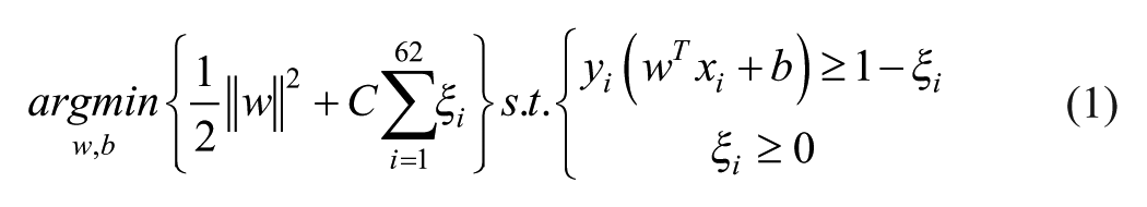
where
To solve the problem reported in Equation 1, one needs to know C beforehand. To estimate the best value of C, we used four-fold cross-validation and a grid search on 10 000 linearly spaced values in the interval
Performance Evaluation
After training, we evaluated model performance according to accuracy on the test set and cross-validation accuracy on the training set. 8 This choice of metrics allowed us to directly compare our results with the state of the art.6,7
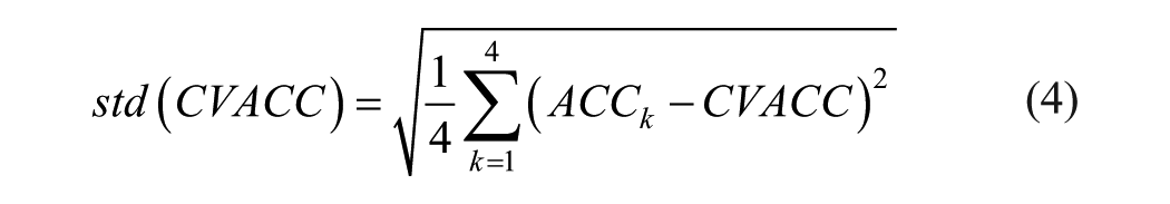
Cross-validation accuracy (

where

and
This way, we can quantify the estimated generalization accuracy, that is, the dependency of prediction quality on dataset composition. Given the limited starting cardinality of our training set, we can expect
This problem is exacerbated by the necessity of two nested cross-validation steps: to evaluate equations 3 and 4, first, we need to reproduce the entire model training and validation phases four times over, including the “inner” cross-validation to select the best value of the hyperparameter in each iteration. However,
Test set accuracy (

This metric summarizes the goodness of classification on the test set, that is, on completely new data that did not have any part in parameter estimation. Hence,
Results
The linear SVM model, based on 17 indices and four basic parameters, reached an
Classification Results.
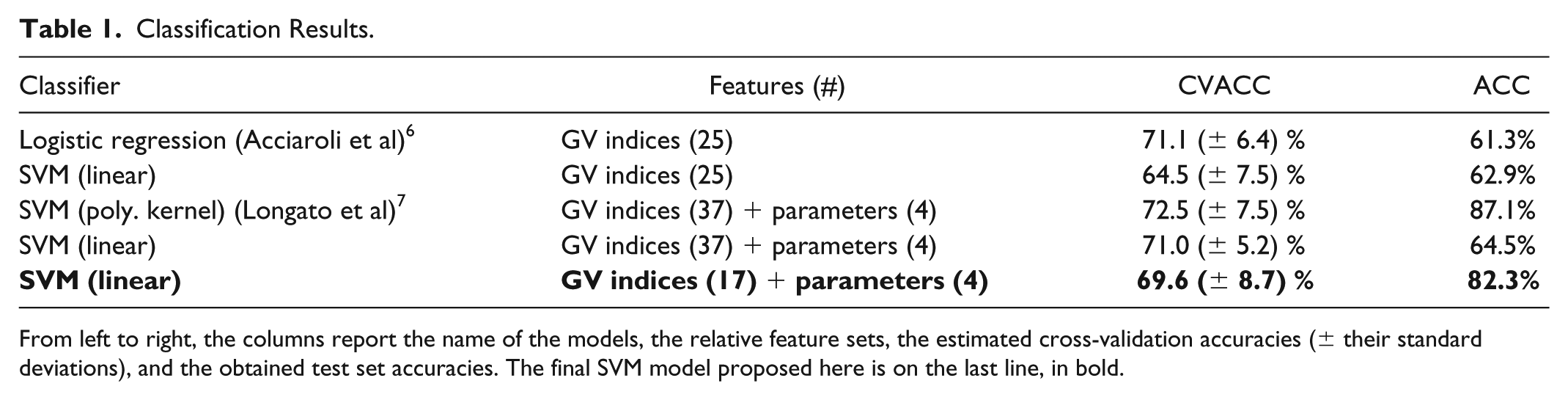
From left to right, the columns report the name of the models, the relative feature sets, the estimated cross-validation accuracies (± their standard deviations), and the obtained test set accuracies. The final SVM model proposed here is on the last line, in bold.
To better understand our final model and, at the same time, comprehensively compare it to the state of the art, we reimplemented it with different feature set configurations. Specifically, we ran it against the 25 GV indices used in Acciaroli et al,
6
and the full set of 37 indices and 4 parameters used in Longato et al.
7
As we can see in Table 1, both experiments yielded unsatisfactory
We also challenged our initial assumption of independence between the first and second visit data (first paragraph of the Classification Strategy section), and split the training and test set in two groups of 16 subjects with two visits each. Although we obtained extremely similar results (
Discussion
There is abundant evidence, in the literature, that diabetes progression and GV deterioration are linked.31-33 Previous works have addressed the problem of using GV indices computed from CGM data to identify different stages of T2D progression. Particularly, to the best of our knowledge, Acciaroli et al 6 is the first report of satisfactory accuracy (91.4%, in a cross-validation scheme) in distinguishing between healthy subjects and those affected by either IGT or T2D using a set of 25 GV indices. Then, Longato et al 7 demonstrated that a further subdivision between IGT and T2D cases, which the authors of Acciaroli et al 6 identified as a critical point of their study, was possible with an accuracy of 87.1%. This promising result, however, came at the cost of ease of interpretation, as it required the implementation of a SVM with a polynomial kernel and the inclusion of 37 GV indices, plus four basic individual parameters.
Here, we simplified the method proposed in Longato et al
7
with the aim of increasing ease of interpretation, while still obtaining comparable, if marginally less accurate, results (
The reduction of the feature space of GV indices is central to the present work, as evidenced by the 33% accuracy increase shown in Table 1 (compare the last and second-to-last rows). This is consistent with previous studies,6,15,34,35 which identified the high degree of correlation between GV indices as a source of detrimental redundancy.
Given the lack of a much-needed consensus on the best subset of indices, feature selection has been investigated in the literature. 19 However, automatic procedures often fail to generate stable results and, to the best of our knowledge, there is no evidence that the most appropriate subset of indices for a given task would translate just as well to another. In light of these considerations, we designed a self-consistent index subset, built with the explicit intention of simplifying the interpretation of our model, as opposed to one automatically generated with the sole purpose of blindly increasing accuracy. While it is true that this choice negatively impacted classification performance by roughly 5% compared to Longato et al, 7 it also removed two extra layers of complexity, that is, the great number of possibly opaque indices and the necessity of kernel-induced nonlinearity.
A limitation of our study is its dependence on the informed, but ultimately subjective, guidance of an expert diabetologist. To reduce this possible bias, the clinician evaluated all the GV indices in the same session, without seeing actual comparisons of IGT versus T2D CGM traces. In this way, he could focus on selecting a subset of indices based on their interpretability and not on the ramifications of his choices in terms of classification. Furthermore, we note that it is not uncommon to involve physicians in sensitive parts of the model development and performance evaluation phases (eg, in Marling et al, 21 the authors set the labels of their study based on the input from two medical practitioners).
Another limitation is the suboptimal duration of the CGM recordings at our disposal. Previous works have shown that, to obtain reliable GV index estimates, we would require 12-15 days of data.36,37 Nevertheless, given our satisfactory results, this issue did not seem to unduly influence classification performance.
Conclusion
The present research investigates whether a suitable subset of CGM-based GV indices can be used to recognize different stages of diabetes progression. In previous contributions, we showed that logistic regression can distinguish healthy subjects from those affected by either IGT or T2D (91.4% CVACC);
6
and that more indices, four basic parameters (age, sex, BMI, and waist circumference), and a complex machine learning technique enable to pinpoint the exact metabolic state between IGT and T2D.
7
In the present article, we aimed at streamlining the latter process by reducing the number of considered indices and using a simpler model. Particularly, after selecting a subset of 17 indices and the same four basic parameters used in Longato et al,
7
we demonstrated that a linear SVM can classify IGT and T2D cases with satisfactory accuracy (
Building a subset analogous to the one we used here could help avoid black-box approaches that might prove controversial, thus, possibly, narrowing the gap between complex state-of-the-art models and more approachable techniques. Hopefully, this would, in turn, favor the incorporation of such methods in routine clinical practice.
Future work will involve the analysis of a completely new dataset, comprising subjects across all stages of diabetes progression. Access to such data would be instrumental not only in validating this and other methods, but also in comparing automatic versus manual feature selection techniques to determine the relative importance of each GV index. Another possibility would be to combine CGM-extracted GV indices with other signals or laboratory tests, and evaluate the trade-off between model interpretability and acquisition cost.
Footnotes
Acknowledgements
Abbreviations
ACC, accuracy; ADRR, average daily risk range; BG, blood glucose; BGRI, blood glucose risk index; BMI, body mass index; CGM, continuous glucose monitoring; CONGA, continuous overlapping net glycemic action; CV, coefficient of variation; CVACC, cross-validation accuracy; EF, excursion frequency; GRADE, glycemic risk assessment diabetes equation; GV, glycemic variability; HBGI, high blood glucose index; IGC, index of glycemic control; IGT, impaired glucose tolerance; IQR, interquartile range; LBGI, low blood glucose index; MAGE, mean amplitude of glycemic excursions; MODD, mean of daily differences; SD, standard deviation; SDd, SD of daily means; SDw, mean of daily SD; SVM, support vector machine; T2D, type 2 diabetes.
Declaration of Conflicting Interests
The author(s) declared no potential conflicts of interest with respect to the research, authorship, and/or publication of this article.
Funding
The author(s) received no financial support for the research, authorship, and/or publication of this article.