
Abstract
Background:
Tens of glycemic variability (GV) indices are available in the literature to characterize the dynamic properties of glucose concentration profiles from continuous glucose monitoring (CGM) sensors. However, how to exploit the plethora of GV indices for classifying subjects is still controversial. For instance, the basic problem of using GV indices to automatically determine if the subject is healthy rather than affected by impaired glucose tolerance (IGT) or type 2 diabetes (T2D), is still unaddressed. Here, we analyzed the feasibility of using CGM-based GV indices to distinguish healthy from IGT&T2D and IGT from T2D subjects by means of a machine-learning approach.
Methods:
The data set consists of 102 subjects belonging to three different classes: 34 healthy, 39 IGT, and 29 T2D subjects. Each subject was monitored for a few days by a CGM sensor that produced a glucose profile from which we extracted 25 GV indices. We used a two-step binary logistic regression model to classify subjects. The first step distinguishes healthy subjects from IGT&T2D, the second step classifies subjects into either IGT or T2D.
Results:
Healthy subjects are distinguished from subjects with diabetes (IGT&T2D) with 91.4% accuracy. Subjects are further subdivided into IGT or T2D classes with 79.5% accuracy. Globally, the classification into the three classes shows 86.6% accuracy.
Conclusions:
Even with a basic classification strategy, CGM-based GV indices show good accuracy in classifying healthy and subjects with diabetes. The classification into IGT or T2D seems, not surprisingly, more critical, but results encourage further investigation of the present research.
Keywords
The concept of glycemic variability (GV) is broadly used in diabetes context to characterise the fluctuations of blood glucose (BG) profiles, which are often involved in the pathogenesis of diabetes-related complications.1-8 Tens of different metrics were proposed in the literature to quantify the GV, including indices derived from the distribution of glucose readings or the amplitude and duration of the glycemic excursions, indices based on risk and quality of glycemic control, just to name a few (see Ohara et al, 8 Rodbard, 9 Le Floch and Kessler, 10 Kovatchev and Cobelli 11 ).
The GV concept has become even more intriguing since the advent of continuous glucose monitoring (CGM) sensors. These sensors measure glucose concentration every 1-5 minutes for several consecutive days, allowing the characterization of the dynamic properties of BG profiles by capturing components otherwise invisible with the traditional self-monitoring of blood glucose (SMBG) management. 11 GV indices computable from CGM traces12-16 have been used in several studies to assess the impact of GV on the risk of developing some diabetes complications,17-19 to quantify the quality of the glycemic control, 20 and to stratify CGM traces in relation to the need of therapeutic actions. 21
Recently, several studies employed CGM technology not only in the population with diabetes,22,23 but also in subjects affected by states of prediabetes and in obese individuals,24,25 where a progressively increasing GV as moving from normal subjects to subjects with prediabetes has been observed. 26 Such progressive changes in glucose dynamics in different categories of subjects suggest that GV metrics extracted from CGM signals could be used to detect impaired glycemia in certain groups of subjects 27 much earlier than the standard techniques used for the diagnosis and classification of diabetes, based on oral glucose tolerance test (OGTT) and HbA1c values. 23
The problem of how to best exploit the plethora of GV indices to distinguish among different categories of subjects is still debated since there are unresolved issues like, for example, GV indices that carry on redundant information.28,29 In this context, even a basic question like using GV indices to automatically recognize if a subject is healthy rather than affected by a state of prediabetes, such as impaired glucose tolerance (IGT), or by type 2 diabetes (T2D), is still unaddressed in the literature to the best of our knowledge.
In the present work, we use a machine learning approach to distinguish healthy from IGT&T2D and IGT from T2D subjects using a set of 25 well established CGM-based indices.
Methods
Database
The data set consists of 102 subjects belonging to three different classes, preliminary determined for each individual by a standard OGTT: 34 healthy subjects, 39 IGT subjects, and 29 T2D subjects (IGT and T2D subjects participated in the Botnia Study in Finland, approved by the Ethics committee of the Helsinki University Hospital with informed consent from all study participants). Each subject was monitored by either the Guardian Real Time or the iPro CGM systems (Medtronic MiniMed, Inc, Northridge, CA) under normal life conditions for an average period of 5 days. Figure 1 shows an exemplificative CGM trace for each of the three categories (healthy subject in the first panel, IGT subject in the second panel, and T2D subject in the third panel).
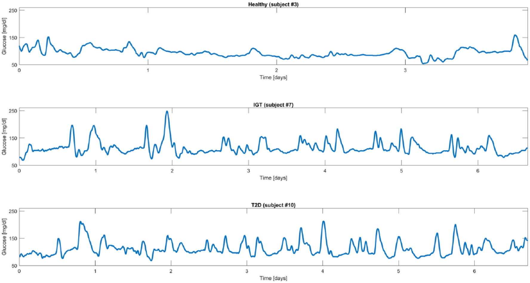
Representative CGM traces from representative healthy (first panel), IGT (second panel), and T2D (third panel) subjects.
Indices Used for Classification
The 102 CGM traces were first processed to extract the set of well-established 25 indices already considered in two recent studies by Fabris et al.28,29 Each GV index has been mean-centered and scaled before entering the classification procedure. The pool of indices comprises metrics based on statistical properties, that is, standard deviation (SD), coefficient of variation (CV), range, interquartile range (IQR), and J-index, 30 indices based on interday variability of statistical properties, that is, mean of daily SD (SDw) and SD of daily means (SDdm), 14 indices based on the permanence in the euglycemic target range, that is, percentages of values below the target range (<70 mg/dL), above the target range (>180 mg/dL) and within the target range ([70, 180] mg/dL), indices related to significant glycemic excursions, that is, mean amplitude of glycemic excursions (MAGE) index,31,32 and measures derived from nonlinear transformations of glucose values, that is, low and high blood glucose indices (LBGI, HBGI),33,34 blood glucose risk index (BGRI), 35 average daily risk range (ADRR), 36 hypoglycemic index, hyperglycemic index and index of glycemic control (IGC), 15 glycemic risk assessment diabetes equation (GRADE) score with its three different glycemic states (%GRADEhypo, %GRADEeu, %GRADEhyper), 37 and, finally, the M100 index. 38 In addition, the pool of indices comprises mean and median glucose. While, from a certain point of view, these two indices are not exactly related with the concept of “variability,” they are normally included in the tools used for glucose time-series analysis.28,29 Therefore, for the sake of reasoning, in the reminder of the present work all the above-mentioned indices will be referred to as GV indices. The correlation among the indices in the considered sample of subjects is briefly commented at the end of the appendix.
Classification Strategy Overview
The proposed classification system is based on a logistic regression model. 39 In particular, to assign each subject to a class, a two-step binary logistic regression model is implemented. The first step aims to distinguish healthy from subjects with diabetes (obtained merging IGT and T2D classes). At the second step, all subjects assigned to the IGT&T2D group at the previous step are classified into IGT or T2D.
The two classifiers are trained on a subset of the 25 GV indices (specific for each of the two classification steps) that best distinguish between classes, that is, the subset of features that guarantee higher classification performance, as determined by a feature-selection algorithm. In particular, the subset of indices that best correlate with classification performance automatically selected by the feature selection procedure is composed of 8 over 25 indices for the first classification step, and 5 over 25 indices for the second classification step (see the appendix for details).
In our experiments, the classifier is trained using a stratified 5-fold cross-validation approach in which the data set is subdivided into five equally sized folds where the proportion of heathy, IGT and T2D subjects in each fold reflects the distribution in the entire data set. Iteratively, one of the five folds composes the test set, used to evaluate classification performance, while the remaining four folds are used to train the classifier. In this way, we guarantee independence between training and test of the classifier and fairness of the results. Training and test phases are briefly described in the following sections.
Training Phase
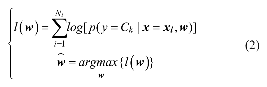
During the training phase, the set of 25 GV indices and the class label of each subject are used to build the classifier. The logistic regression model we used in the experiments can be expressed by the following formula:
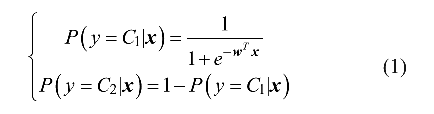
where
where
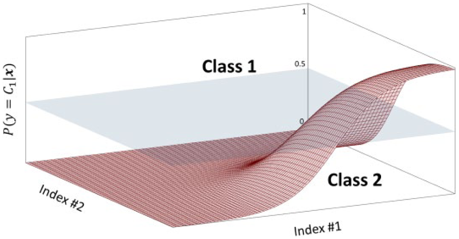
Simplified representation of sigmoid function with n = 2 dimensions. The sigmoid surface divides the probabilistic space into two areas, corresponding to the two classes.
Test Phase
The test phase is used to evaluate classification performance on an unseen subset of subjects, that is, the test group. In particular, the set of GV indices
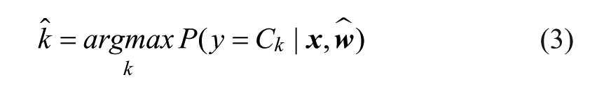
Practically, in relation to the graphical representation of Figure 2, solving Equation 3 corresponds to: look at the vector of coordinates
Assessment Criteria
Classification performance is quantified by comparing the class predicted by the classifier,
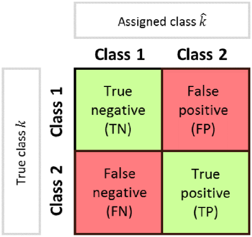
Scheme of confusion matrix for the evaluation of classification performance.
Accuracy:
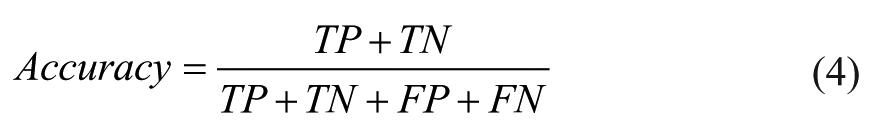
that represents the fraction of subjects correctly classified among the total number of subjects examined.
Precision:
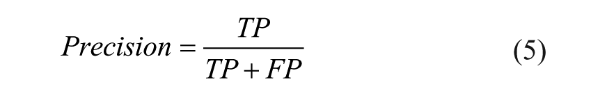
that is, the fraction of TP among the total number of positives. It gives intuitively the ability of the classifier not to label as positive a sample that is negative.
Recall:
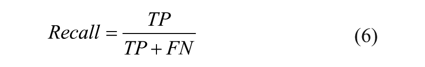
that is, the fraction of TP among the sum of TP and FN (the total number of elements of that class), which intuitively measures the ability of the classifier to detect all the positive samples.
F1 score:
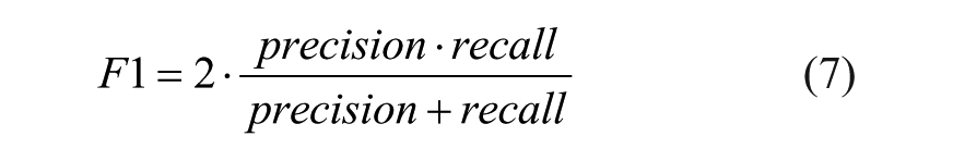
that represents the harmonic mean of precision and recall. Its value is between 0 and 1, where 0 and 1 indicate, respectively, poor and good classification performance.
Results
Attained 5-fold cross-validation results are shown in terms of accuracy in Table 1, where we reported mean and SD among the five cross-validation folds. In particular, the first classification step distinguishing healthy from subjects with diabetes (comprising both IGT and T2D classes) has mean accuracy of 91.4% with 9.8% SD, whereas the second classification step, which further distinguishes between IGT and T2D, has mean accuracy of 79.5% with 15.9% SD. The global classification into the three classes shows mean accuracy among the five folds of 86.6% with 11.7% SD.
Classification Accuracy (First and Second Classification Steps and Global Result).
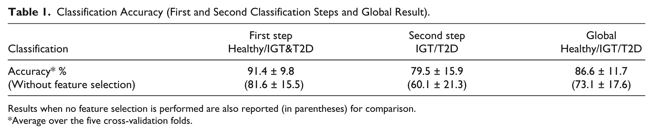
Results when no feature selection is performed are also reported (in parentheses) for comparison.
Average over the five cross-validation folds.
A deeper analysis of classification performance is done by quantifying the number of subjects correctly and wrongly classified at each step. At the first classification step, 4 healthy subjects are wrongly classified as subjects with diabetes (IGT&T2D) and 7 subjects with diabetes are wrongly classified as healthy, while all other 91 subjects are correctly classified. At the second classification step, that is applied in cascade to the first one, 5 IGT subjects are wrongly classified as T2D, 7 T2D subjects are wrongly labeled as IGT, while all the other 49 subjects are correctly classified.
In Table 2, we reported precision, recall, and F1 score for each of the three classes: healthy (second column), IGT (third column), and T2D (fourth column). Precision and recall are computed in percentage, showing values above 80% for all the three classes, whereas the F1 score, which can vary between 0 and 1, is greater than 0.8 for all the three classes.
Precision, Recall, and F1 Score (Healthy, IGT, and T2D Classes).
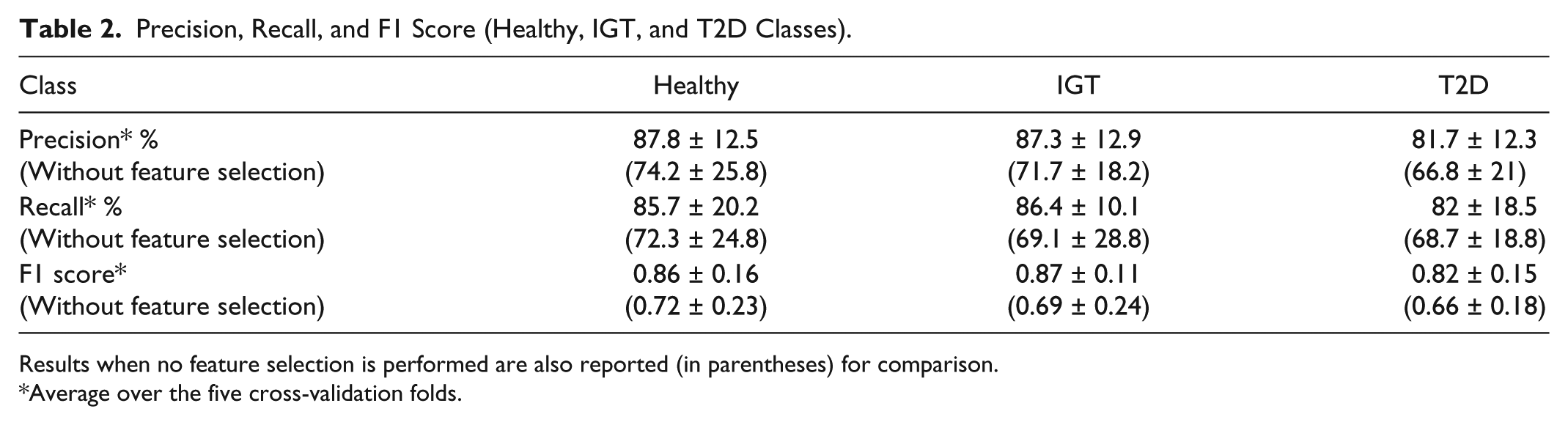
Results when no feature selection is performed are also reported (in parentheses) for comparison.
Average over the five cross-validation folds.
In both Table 1 and Table 2, we also reported the classification performance obtained when no feature selection is performed, that is, when the classifiers are trained on the complete set of 25 GV indices. This analysis is performed and documented to emphasize the relevance of the feature selection process. Indeed, all performance metrics result lower when compared to that obtained after the feature selection process.
Discussion
A first aspect to be noted from Table 1 is that the subdivision of the subjects between healthy and subjects with diabetes (comprising both IGT and T2D classes) is much more accurate than the subsequent subdivision of IGT&T2D into IGT or T2D. Results of the first classification step ensure that we are able to correctly distinguish between normal and pathologic condition in nine cases over ten. This result appears even more interesting if one notes that the subjects of the healthy group present a mean BMI of 30.01 kg/m2 at limit with obese status. On the other hand, the further classification between IGT and T2D subjects appears less effective, with mean accuracy of 79.5%. Analyzing the structure of the classification problem, which is a two-step procedure, we note that the second classification step suffers from error propagation. Indeed, subjects that are wrongly classified by the first classification step, that is, healthy subjects that are labeled as subjects with diabetes will obviously result in errors also in the second classification step. However, all the other metrics shown in Table 2 (precision, recall, and F1 score) are substantially stable among the three classes with values always above 80%.
The second interesting aspect is the outcome of the feature selection, which, for the first classification step, is composed of the following 8 indices: mean, CV, range, percentage of values below target, percentage of values within target, HBGI, ADRR, and BGRI; and for the second classification step is composed of the following 5 indices: median, SD, CV, MAGE, LBGI. In fact, on one hand, the analysis of these two subsets of indices confirms the high redundancy carried by the original set of 25 GV indices, as already observed in Fabris et al,28,29 whereas, on the other hand, evidences the specificity of each index in describing particular characteristics of the glucose dynamics. Indeed, the two subsets have no overlap, with the exception of CV, a standard statistical feature that is powerful to assess glucose variability 40 and appears useful for both classification steps when combined with more specific GV metrics. This aspect suggests that more class-specific indices could be included in the set of features that serves as input to the machine-learning algorithm, with the aim of improving class-to-class subdivision.
Conclusions
Tens of GV indices were proposed in the literature, even more since the advent of CGM sensors, and used for several purposes, such as to quantify the quality of glycemic control or to assess the risk of developing diabetes-related complications, but their usability and reliability for classification problems is still scarcely investigated.
In the present work, given a data set of 102 subjects, we analyzed the performance of an automatic classifier that distinguishes between healthy, IGT, and T2D subjects using GV metrics extracted from CGM traces. Results confirm that CGM-based GV indicators can effectively distinguish CGM traces of healthy and subjects with diabetes (IGT&T2D), with an overall mean classification accuracy of 91.4%. The subdivision of subjects into IGT or T2D appears, not surprisingly, more critical, but results (79.5% accuracy) encourage further investigation of the present research. Furthermore, the global subdivision into the three classes shows 86.6% accuracy.
Future developments will consider the application of the classification algorithm to different and possibly larger data sets that could permit the construction of more robust classifiers, as well as the implementation of different, more sophisticated machine-learning techniques. Possibly, inputs of the classification algorithms could also be extended by adding other different GV indices and, if available, some basic clinical parameters (eg, age, height, weight) that could further improve the GV indices-based classification performance.
Footnotes
Appendix
When dealing with classification problems, it is important to check whether all available information is actually needed to efficiently solve the problem. In general, it is good practice to reduce the set of features that describe the object by removing the “noisy” features that are not crucial (or even that influence negatively) for distinguishing between the considered classes.
Here, we analyze if the whole set of features, that is, the complete set of 25 GV indices, is actually needed to distinguish between classes, or if it is instead possible to reduce it by selecting a specific subset of indices. This problem can be solved through many feature selection methods. In this article, we used a forward sequential feature selection (SFS) approach.
41
The forward SFS method finds the best subset
This procedure is run at each of the five cross-validation iterations by subdividing the training set into actual training part and validation part (following an 80% to 20% partition rule). The training part is used to build the different classifiers (point 2.1.1 in the algorithm above) and the validation part is used to compute the performance measure (here given by the F1 score on the validation group). The features selected by the SFS nested in the cross-validation scheme are quite stable among the folds, that is, many features recur in the five subsets while few others appear to depend on the training set. The global output of the SFS reported in the Discussion section is instead obtained on the entire data set.
For sake of completeness, we report in Table A1 the correlation matrix of the 25 GV indices estimated from the considered data set. It clearly shows that indices are somehow mutually related. Interestingly, compared to the same matrix reported by Fabris et al 29 for a homogeneous population of T2D subjects, here lower correlation coefficients are found, because of the greater heterogeneity of the subjects (healthy, IGT, and T2D).
Acknowledgements
Abbreviations
ADRR, average daily risk range; BG, blood glucose; BGRI, blood glucose risk index; CGM, continuous glucose monitoring; CV, coefficient of variation; GRADE, glycemic risk assessment diabetes equation; GV, glucose variability; HBGI, high blood glucose index; IGC, index of glycemic control; IGT, impaired glucose tolerance; IQR, interquartile range; LBGI, low blood glucose index; MAGE, mean amplitude of glycemic excursions; OGTT, oral glucose tolerance test; SD, standard deviation; SDw, mean of daily SD; SDdm, SD of daily means; SFS, sequential feature selection; SMBG, self-monitoring of blood glucose; T2D, type 2 diabetes.
Authors’ Note
The present study has been presented in preliminary form at the 16th Annual Diabetes Technology Meeting, November 10-12, 2016, Bethesda, MD, with the work titled “Good Accuracy of CGM-Based Glucose Variability Indices for IGT and T2D Classification,” by Acciaroli et al, winning the Gold Prize of the Diabetes Technology Society Student Research Award.
Declaration of Conflicting Interests
The author(s) declared no potential conflicts of interest with respect to the research, authorship, and/or publication of this article.
Funding
The author(s) disclosed receipt of the following financial support for the research, authorship, and/or publication of this article: This study was performed as part of the FP7-MOSAIC project funded by the European Union under the 7th framework program (grant agreement FP7-600914). The Botnia Study has also been financially supported by grants from the Sigrid Juselius Foundation, Folkhälsan Research Foundation, Ollqvist Foundation, Signe and Ane Gyllenberg Foundation, Swedish Cultural Foundation in Finland, Finnish Diabetes Research Foundation, Foundation for Life and Health in Finland, Helsinki University Central Hospital Research Foundation, Närpes Health Care Foundation, and Ahokas Foundation.