Sage Journals: Discover world-class research

Abstract

Background:

Current methods used to assess glycemic control use averaged measures and provide little information on the glycemic pathology of the patients. In this article we propose visual tools and their related mathematical formulas that allow for improved characterization of the glycemic behavior and achieve better glycemic control.

Methods:

We present a reanalysis of published data, based on SMBG measurements from clinical trials of both men and women older than 18 years who were either healthy volunteers, prediabetes, or type 1 or type 2 diabetes. New graphic visualizations of glycemia as well as mathematical formulas that describe the glycemic behavior are presented and described, as well as suggested methods for their use to improve glycemic control.

Results:

Patients with different problems in their glycemic control had different histogram shapes. In addition, patients who had the same HbA1c level at the time of the trial revealed significantly different glucose histograms with different shapes, variability and glycemic burden. The derived graphic visualizations provided information about the temporal evolution of the glycemic control.

Conclusions:

A paradigm change of the existing model of diabetes control is proposed, shifting from standardized treatment algorithms based on HbA1c follow-up to a new controlling approach that is based on the personal glucose density histogram. The histogram is an informative, detailed tool for the current patient glycemic behavior, and a future histogram can be targeted for a successful treatment. In addition, the glucose burden and the glucose severity index are proposed as informative markers for successful treatment. This is applicable to any glycemic data, by means of invasive and noninvasive glucometers.

Keywords

glycemic burden glycemic severity index glucose histograms personalized medicine diabetes care Hb-A1c

Once a patient is having diabetes, the clinical outcome is inherently linked to the patient’s lifestyle, especially in type 2 diabetes; together with the large variability of individual metabolism, it is being increasingly recognized that effective treatments need to evolve beyond our current treatment models toward personalized ones, in order to provide improved quality of life and better long-term outcomes.^1,2 One of the most appealing approaches to meet this goal within health care economic constrains and in light of the evolution of our societies into the digital age is to implement informatics into our diabetes care systems. When digital modalities are used as add-ons to the current system their contribution to outcomes and costs seems to be only modest.^3,4 When digital approaches are part of an integrated care system they provide better outcomes, and the lower the baseline level of health care (for different reasons—attitude, knowledge, economics, access, etc), the more there is to gain.^5,6 In order to obtain the benefits of telemedicine and computerized decision aids, these need to be customized around the specific problem, in the specific setting, for the specific population.⁷ Patient empowerment as a general intervention alone does not seem to be enough;⁸ the digitalization of diabetes care needs to be coupled to the patients’ actual data and care specifics, in order to provide a relevant, positive feedback loop that encourages further engagement.^9,10 Therefore, for diabetes care to successfully embrace digital health technologies, evolution is not enough; we need a revolution of our paradigms of delivery and utilization of care. In this context, the provision of patient-level data emerges as a crucial point in the quest for better, personalized diabetes care that makes economic sense.

The most commonly used method for detecting and controlling diabetes status is by measuring HbA1c. However, as an average value, it doesn’t give the full picture of the patient glycemic behavior¹¹ or give an indication on the individual patient’s metabolism, among other problems,¹² such as different rates of glycosylation in different people,¹³ ethnic variability in the correlation between glycemic burden and HbA1c levels.¹² Thus, it stands to reason that analyzing the actual glycemic behavior using data from intensive (self-) monitoring would be preferable. Indeed, the frequent self-monitoring of blood glucose has been shown to improve diabetes management,¹⁴ but intensive self-monitoring using invasive procedures (ie, finger lancets and glucose strips) is impractical on the long term. The use of continuous glucose monitors, which have been shown to improve outcomes,¹⁵ is an appealing alternative, but they also have drawbacks such as having been tested mainly in type 1 diabetes, requiring high compliance to show significant benefit, having biocompatibility problems, requiring the attachment of implantable sensors, and having significant economic costs.^16-21

Noninvasive glucose measuring technologies are coming of age, among them the TensorTip Combo Glucometer (CoG) developed by our company.²² Noninvasive devices allow patients to measure themselves with less discomfort or pain, as well as being able to do repeated, frequent measurements for intensive monitoring. Still, obtaining the data is not enough, since the large amounts of data generated by frequent monitoring is not always interpreted and exploited properly, and physicians and patients alike can struggle to make practical use of it.^17,19,20

This article presents a novel way to analyze and interpret longitudinal glycemic data, centered on the use of a temporal density glucose histogram together with the novel metrics, glycemic burden (GB) and glycemic severity index (GSI), as the measures and control indexes for diabetes.

Materials and Methods

Study Device

All data and histograms in this study are based on the measurements of the CoG (Cnoga Medical Ltd, Caesarea, Israel) device which is approved in Europe (CE), Brazil, China, Israel, and other countries, and is intended for invasive and noninvasive glucose monitoring for domestic use or as an additional support in clinics.²² In this article the invasive readings of the CoG were in the range of 40-500mg/dL and were obtained from lancing a fingertip. This add-on invasive module is identical to the Okmeter match device K090609 (OK Biotech Co, Ltd, Hsinchu City, Taiwan). The noninvasive unit is based on the TensorTip optical technology developed by Cnoga. The device uses 4 light-emitting diodes of different wavelengths for excitation and a high speed CMOS color image sensor, using Cnoga’s proprietary algorithms, it measures instantaneously and noninvasively the tissue glucose.

Statistical Methods

The glycemic data were obtained from men and women older than 18years that were either healthy volunteers, prediabetes, type 1 or type 2 diabetes, using the CoG. The data were prepared using Excel (Microsoft, WA, USA); the statistical analysis and figures were prepared using Python (version 3.5) and JMP Pro (version 13.2.1, SAS Institute, NC, USA). All data have been deidentified.

The raw data used for Figures 2, 3, and 6 come from a previously published report. Briefly, the participants were tested during an open label, prospective, single-center trial, which was conducted in Germany according to local regulations, including informed consent.²³ The data were collected for 10 to 45days, depending on the arm of the trial, during which the patients checked their glucose levels several times per day. Figure 4 was prepared using data from a home clinical trial; it was freely provided by users with type 2 diabetes who provided writteninformed consent allowing the use of their data in an anonymous way for research and development purposes. Figures 1 and 5 were computer generated.

The mathematical measures GB and GSI were developed to objectively characterize the histograms. Their formal definitions and all detailed calculations are presented in the supplementary materials and methods. Briefly, without using mathematical definitions, the GB in its simplest form is the glucose average; it has a specific name since it is defined in such a way that it can be manipulated to give different weights to different parts of the glucose scale. For simplicity, throughout this article, the GB is equivalent to the average. The GSI represents glycemic severity, and is composed of four different measures of variability. The $\bar{G B}$ (“GB bar”) is the weighted distance of the GB from an optimal GB of 100mg/dL; it serves to measure how far is the GB (the average glucose) from the ideal glucose average. $φ$ (phi) is the weighted average deviation of each measure from 100mg/dL. That is, every glucose reading is compared to 100mg/dL, weighted, and all of the readings are averaged. This is a sensitive measure of the deviation of the individual values from the norm, and serves as a complement to the deviations of the averages, represented by $\bar{G B}$ as described above. This is important because a person with high and low glucose readings would have an average that underestimates the severity of his derangement, that is, his $\bar{G B}$ would be better than his $φ$ . $φ$ can be thought of as roughly similar to the variance ( $φ$ also has the potential to be scaled for different patients, but that is beyond the scope of this article). F_H is a measure of how many peaks are there in the histogram. Finally, F_T is a measure of the temporal frequency of the glucose readings over time, that is, how many times the glucose readings change direction over time; it represents the “jumpiness” of the data, as in brittle diabetes for example. Thus, the GSI, which includes of all these four metrics, incorporates the most important measures of glycemic variability: on average ( $\bar{G B}$ ), per individual reading ( $φ$ ), cumulatively (F_H), and over time (F_T). Given that glycemic variability has been shown to be an independent risk factor for diabetes complications^24,25 and a target for diabetes care,^26,27 the GSI is an important measure for diabetes control.

Results

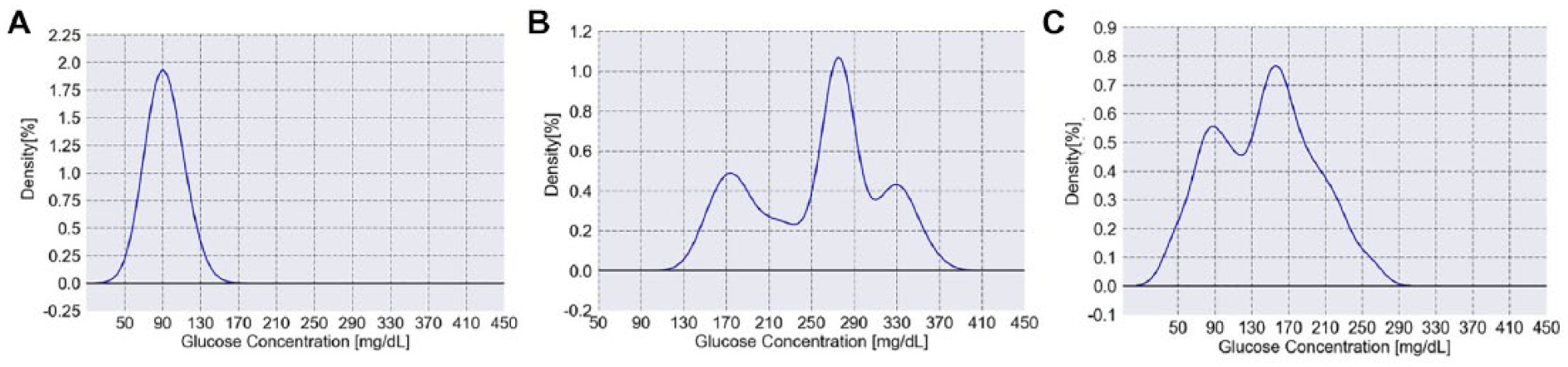
To better understand the glycemic behavior of the patients, the glucose levels can be plotted using a histogram, which allows to discern the underlying distribution of the glucose values. For example, Figure 1A shows a computer-generated histogram that represents the expected behavior of a healthy individual with a GB of 92mg/dL and a GSI of 1.45. Figure 1B represents a severely unbalanced type 2 patient having a GB of 256mg/dL and a GSI of 6.33, with overall elevated glucose levels and a tri-modal distribution. Figure 1C represents a labile type 1 patient having a GB of 144mg/dL and a GSI of 3.76. This patient suffers from several episodes of both hypo- and hyper-glycemia (22% of the readings are equal to or below 80mg/dL and 19% of the readings are equal to or above 200mg/dL).

Figure 1.

Typical histograms representing the glucose distribution of (A) healthy individual with a GB of 92mg/dL and GSI of 1.45 ( $φ$ =1.13, $\bar{G B}$ =1.08, $F_{T}$ =1.39, $F_{H}$ =1). (B) An uncontrolled type 2 patient with GB of 256mg/dL and GSI of 6.33 ( $φ$ =1.59, $\bar{G B}$ =1.61, $F_{T}$ =1.49, $F_{H}$ =1.67). (C) A labile type 1 patient with GB of 144mg/dL and GSI of 3.76 ( $φ$ =1.34, $\bar{G B}$ =1.30, $F_{T}$ =1.44, $F_{H}$ =1.5).

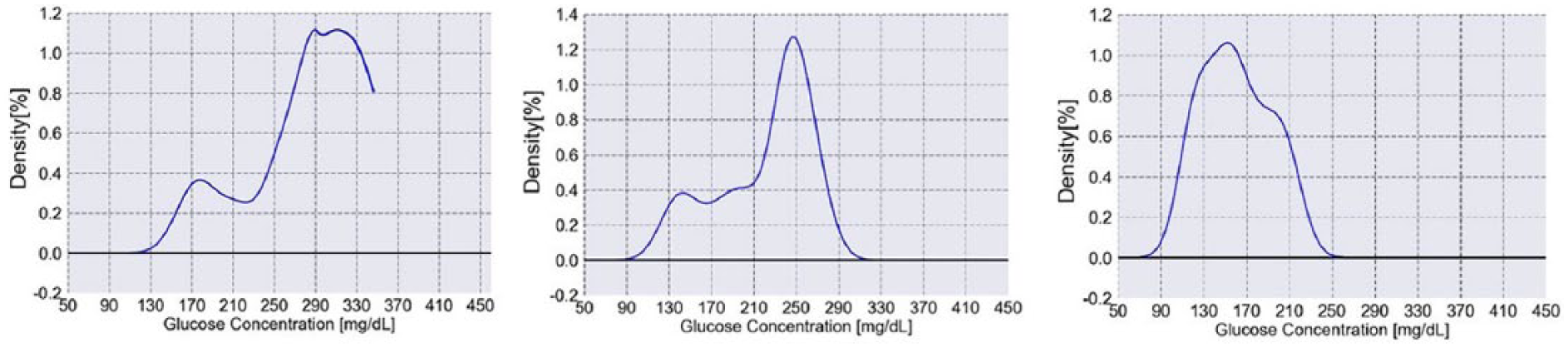
Supplemental Figure 3s shows more examples of glucose distributions corresponding to different conceptual patients, all based on observations from clinical trials previously conducted. These theoretical histograms have a direct relation to the ones obtained when using data from actual patients. For example, Figure 2A shows the distribution of glucose values from an actual patient, that is relatively Gaussian in shape, with a GB of 145mg/dL and three values that are above 180mg/dL; this patient has slightly elevated glucose levels overall but the distribution shape is not abnormal. Figure 2B shows a patient with a bimodal distribution, with the first peak having relatively normal levels and a second peak at 209mg/dL. Figure 2C shows a Gaussian distribution that is both broad, with a high variability, and shifted to the right with a GB of 252mg/dL. Finally, Figure 2D shows an almost flat distribution with GB of 250mg/dL. The detailed parameters of Figure 2 are shown in Supplemental Table 1. Evidently, the patients shown in Figure 2 have very different problems in their glycemic control; such detailed information cannot be observed from a single HbA1c level. Thus, the temporal density glucose histogram is a useful and intuitive way to describe and understand a patient’s glycemic behavior. It is important to note that these histograms are representative when they are obtained using at least five glucose readings per day and optimally eight glucose readings per day: at awakening, before breakfast, after breakfast, before lunch, after lunch, before dinner, after dinner, and before bed time, for at least two weeks, as suggested for other applications.^27,28

Figure 2.

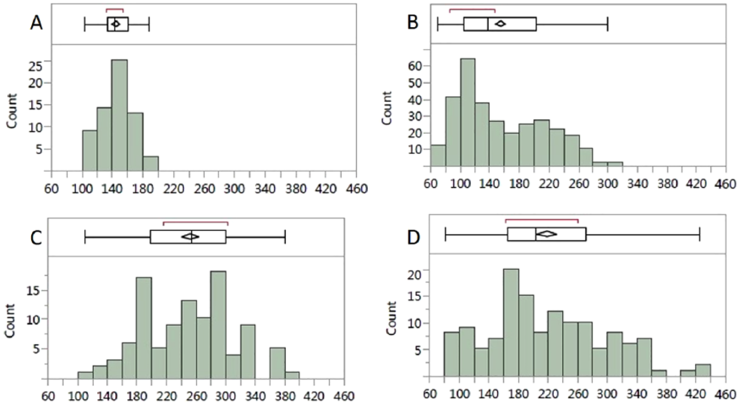
Glucose histograms of actual patients with type 2 diabetes over two weeks of measurements (A-D). The vertical line within the box represents the median sample value. The confidence diamond shows the mean value (the middle of the diamond), while the right and left points of the diamond represent the upper and lower 95% confidence of the mean estimate. The ends of the box represent the first (25th) and third (75th) quartiles, encompassing between them the interquartile range. The whiskers extend from left to right from the first quartile − 1.5. (interquartile range) to the third quartile + 1.5. (interquartile range). The points outside represent to outlying values. The red bracket outside of the box identifies the shortest half, which is the most dense 50% of the observations. The detailed measurements are shown in Supplemental Table 1.

Figure 3A presents three different patients who had the same HbA1c level at the time of the trial, 6.5%, yet their glucose histograms are significantly different, with different shape, GB, and GSI. Similarly, Figure 3B shows three different patients with an HbA1c level of 8.8% to 9% but very different histograms.

Figure 3.

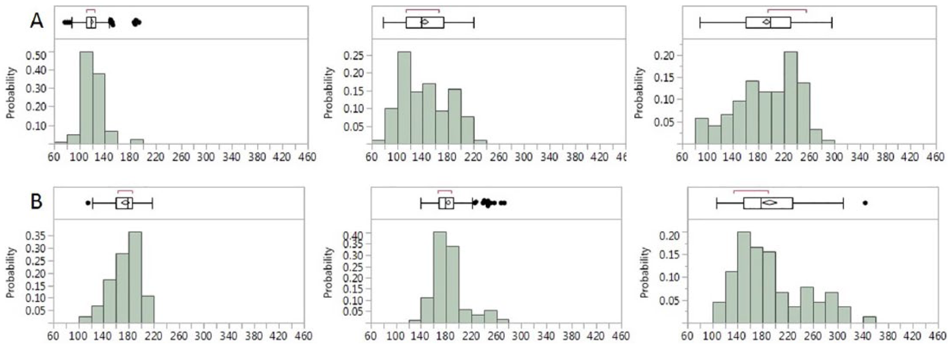
Three representative patients with type 2 diabetes with very different glucose histogram but the same HbA1c level of (A) 6.5% and (B) 8.8% to 9%. The box and whiskers plot are the same as in Figure 2. The detailed parameters are shown in Supplemental Table 2. Measurements done over two weeks.

Figure 4A illustrates the dramatic change in the glycemic behavior of a patient as she entered an intensive glucose control program with the help of the CoG (a change too fast to be reflected in the HbA1c). Figure 4B illustrates a second patient’s histogram four months apart; although at first glance the two histograms look similar, the statistics clearly show a loosening of glycemic control, with all measures shifting 20mg/dL higher. Supplemental Figure 4s demonstrates examples of the evolution over time of the glycemic control of six other patients, as shown through their glucose histograms. The detailed parameters of Figure 4 and Supplemental Figure 4s are shown in Supplemental Table 3. These results imply that the temporal density glucose histogram can be used as a tool to design a desired, target glucose histogram and implement the therapeutic options accordingly. Achieving this desired shape might take a few target cycles, with interim evaluations at every stage. For example, Figure 5 presents a theoretical progression of an uncontrolled type 2 diabetes patient after beginning therapy. At the first stage the GB is 260mg/dLand the GSI is 5.94.

Figure 4.

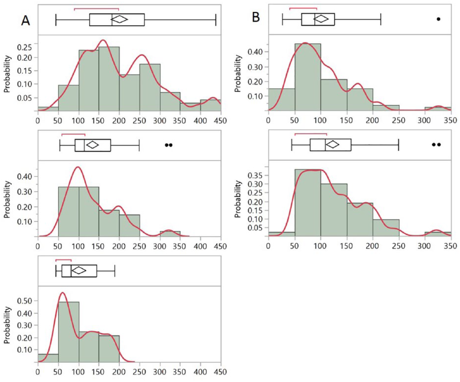
Glucose histograms of type 2 diabetes patients. (A) The top histogram shows the data from one month. Three months later, the patient entered an intensive glucose control program; the middle histogram shows the data from the first two weeks of the program and the bottom histogram shows the data from the second two weeks of the program. (B) The top histogram shows the data from one month. The bottom histogram shows the data from one month, four months later. As the patient relaxes his glycemic control, the mean, median, and interquartile range increase from 89, 101, and 64-127mg/dL, to 109, 124, and 80-159mg/dL respectively. The box and whiskers plot are the same as in Figure 2. The red line is fitted to the actual glucose values underlying the histogram columns. The detailed parameters are shown in Supplemental Table 3.

Figure 5.

Glucose histograms of a prototypical type 2 diabetes patient as he improves his glycemic control. The left histogram shows a skewed distribution with a GB of 260mg/dL and a GSI of 5.94 ( $φ$ =1.59, $\bar{G B}$ =1.60, $F_{T}$ =1.56, $F_{H}$ =1.5), with an estimated HbA1c level of 10.7%. The middle histogram is shifted to the left with a GB of 220mg/dL and a GSI of 5.88 ( $φ$ =1.52, $\bar{G B}$ =1.55, $F_{T}$ =1.67, $F_{H}$ =1.5) with an estimated HbA1c level of 9.29%. The right histogram shows a more Gaussian distribution with fair control of glucose levels, a GB of 160mg/dL and a GSI of 2.93 ( $φ$ =1.36, $\bar{G B}$ =1.38, $F_{T}$ =1.56, $F_{H}$ =1) with an estimated HbA1c level of 7.2%.

The main target of the interventions is to improve the shape of the glucose histogram from a skewed distribution to a more normally shaped one, improving glycemic homeostasis, while also bringing a general reduction of glucose levels. This stage leads to a different histogram shape, together with small improvements in GB that was reduced to 220mg/dL and slight reduction of GSI to 5.88. It is important to note that small change in GSI may still represent a significant progress since it is composed of four separate measures. A second intervention is aimed at shifting the whole distribution toward a lower glucose range and improving the histogram frequency F_H (ie, total peaks) into a single maximum, while avoiding the occurrence of hypoglycemia. In this stage GB was reduced to 160mg/dL and the GSI to 2.93. This stage reflects a major improvement in the severity of his diabetes. Thus, the shape of the histogram and the parameters associated with it (GB and GSI) provide personalized information that can be used to individualize treatment targets and choose between different possible strategies to reach those targets.

The temporal density glucose histogram, as well as other visualizations of glycemic behavior, can help us understand how the glucose levels behave during daily life. This allows us to focus on the most problematic times of the day and target them specifically with behavioral and pharmacological interventions. For example, Figure 6A depicts the distribution of glucose levels for a single type 2 patient during the 24hour daily cycle, encompassing 351 measurements over 2months. It can be clearly seen that the glycemic control is best in the morning, and as the day advances, the glucose histogram becomes more and more skewed. The scatter plot in Figure 6B shows the same data in a different way: as the morning progresses the glucose levels increase up to a peak around lunchtime, with a continuation of these high levels throughout the remainder of the day. The large dispersion of the measures is also noteworthy. Figure 6C depicts a density plot of the same data set, binned into 15minute slots, in what some may find is a more visually intuitive way. This plot focuses on four clear clusters of glucose levels: A, early morning, showing fasting glucose levels of 167mg/dL; B, morning, where glucose levels increase steadily after breakfast; C, a high peak after lunchtime; and finally D, continually high levels from afternoon through the night. Finally, Figure 6D shows a histogram with the different times of day color-coded, allowing us to get a rough sense of the dispersion of values during the day.

Figure 6.

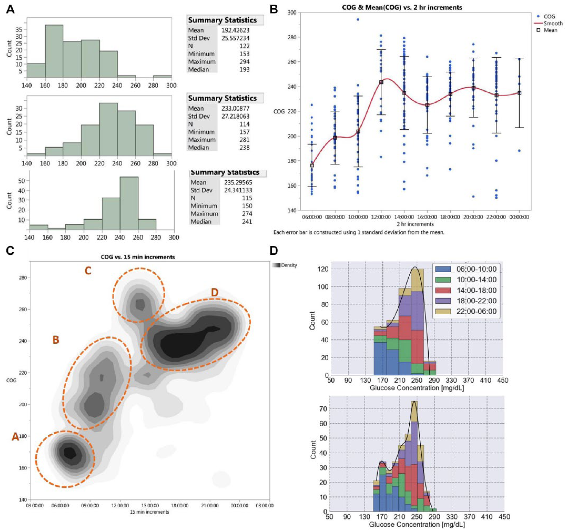
Different distributions of a type 2 diabetes patient over two months. (A) Histograms divided by times of the day, encompassing 351 measurements over two months. The morning histogram (06:00 to 12:00) is on top, the afternoon histogram (12:00 to 18:00) in the middle, and the evening histogram (18:00 to the next morning) at the bottom. The detailed measurements are shown in Supplemental Table 4. (B) The same data are shown, in two-hour increments. The blue dots represent the individual measures, the squares represent the mean glucose value, and the trend is shown in red. The error bars represent ±1 SD from the mean. (C) The same data are shown using a density plot with 15minute increments in the X axis. The density of measurements is shown over 8 gray levels, with the darker areas representing higher density. (D) The same data are shown with stacked histograms, color coded by different hours during the day. The lower histogram shows how the representation changes when the data are plotted using smaller histogram bins.

Discussion

In this article, we explore the use of temporal density glucose histograms as a way to characterize glycemic homeostasis and the therapeutic options afforded by using the histograms, related data visualization, and analysis tools. While histograms have been mentioned in the past²⁹ and some continuous glucose monitors (CGMs) can show a histogram of some of their data, glucose histograms have never been discussed or proposed as a central tool in understanding or managing diabetes. Moreover, tools for their analysis have not been proposed in the past. Therefore, the novelty of our proposed approach is reflected by the elaboration of histograms utilization and their actual implementation, together with their mathematical analysis, as tools for diagnosis, glycemic follow-up, and, importantly, for designing the therapeutic plan for glycemic control. The glucose histogram and derived parameters are device agnostic, being applicable to any scenario where personal glucose data are recorded. The use of these tools allows for significant gains, which feed upon and reinforce each other: improvement upon the use of HbA1c; provision of detailed information on actual glycemic behavior for the personalization care; and ease of understanding and implementing in digital care models.

Beyond HbA1c

The temporal density glucose histogram can improve upon the HbA1c by providing a picture of the actual glycemic derangements. Figure 3 highlights how problematic it is to use the HbA1c as the main indicator of glycemic control in patients with diabetes. Similar HbA1c values can be obtained from very different underlying glycemic behaviors, and “normal” HbA1c levels can be obtained from patients with deranged glucose metabolism. Although useful as a general follow-up measure, the HbA1c is only a very rough estimate of a patient’s state and it is questionable as a reliable way to compare among patients. In contrast, the GB and GSI are standardized and based on the actual glucose measurements, bypassing the “biological interface” that is involved in the creation of the HbA1c molecule. Thus, they are better suited for objective follow-up and epidemiological studies, as well as providing more information than what is represented by the HbA1c.

Personalization of Care

Patients with diabetes are heterogeneous, comprising a spectrum of pathophysiologic configurations,³⁰ requiring therapy tailored to their specific diabetes subtype. A prerequisite to perform this personalization of treatment is to have the individual’s data presented at a level that is detailed enough, a requisite that can be fulfilled by using the temporal density glucose histogram, the GB and the GSI. In principle, the insulin resistance (or an indexed form of it) may also be computed from the glucose histogram if additional information related to medications, food and physical activity is provided. Moreover, it is not only the different histogram shapes but also their change in response to treatment that can greatly help understanding the underlying problems of the patients. The dynamic representation of a patient’s glycemic behavior analyzed over time, as shown in Figure 4 and Supplemental Figure 4s, exemplifies this. These tools can help a clinician devise specific interventions, reinforce a good strategy or modify an inadequate one. The period of analysis can be much faster than is common with HbA1c, as dynamics can be monitored as soon as every two weeks. This allows clinicians to provide relevant, real time feedback and adjust the pharmacologic intervention as the patient changes into a new equilibrium. Figure 5 in turn demonstrates the relation between the GB and GSI values to the severity of the disease. This approach stands in contrast with current treatment guidelines that look at the HbA1c, propose general lifestyle changes mostly for un-medicated type 2 patients and prescribe medications according to a standard flowchart or table when it comes to medicated patients.

The power of graphical tools for glucose data visualization and analysis is further demonstrated when looking at daily glucose patterns, as in Figure 6. These intuitive graphs show the actual glycemic control in the day to day and can be used as the basis for improving glycemic control in relation to patient-specific problem areas. Other types of analyses of daily glycemic data have been described before, prominently the ambulatory glucose profile;^11,29 while some of our tools bear resemblance to it by necessity, since we also show the glycemic behavior over 24hrs, our overall approach is broader, providing several ways to visualize the data and analyze it. From a patient-centered perspective, the proposed glucose visualizations (with the histogram at the center) coupled with the GB and GSI, provide the patients a clear view of the specific areas that need better control (as opposed to general recommendations), and this type of educational interventions have been shown to reduce mortality among patients with diabetes.³¹

Glycemic Variability

Other measures of glycemic variability have been proposed in the past, such as SD, CV%, MAGE, MODD and others.^32,33 The GSI provides several advantages over them: (1) It does not assume normality, since once glycemic homeostasis is lost to diabetes, the glucose distribution quickly loses normality. (2) It incorporates four different measures, each one related to different domains of the variability (as described above). This provides a fuller description of the variability that adds to the ability to correlate it to pathophysiological processes. (3) When used for a specific patient, it can be manipulated to adapt it to the patient’s pathophysiology and reflect more accurately his specific goals of care. (4) Most of the glycemic variability measures existing in the literature are appropriate for continuous, high-resolution data (like what is obtained from CGMs), or for sparser data obtained (such as from flash glucose monitors, SMBG, or noninvasive monitors). In contrast, the GSI can be used for any one of them, as long as enough data points are obtained, regardless of the period of time involved.

Implementation and Health Care Delivery

The temporal density glucose histogram and the associated measures are simple yet powerful tool that can facilitate the implementation of informatics for the care of patients with diabetes.³ By converting data into information and then help extract from the information clinically actionable insights, they can be of use for both health care personnel and patients.

This approach to diabetes control should not be restricted to insulin users. For example, a patient with type 2 diabetes not treated with insulin might, nonetheless, use a noninvasive monitor and do intensive self-monitoring in a convenient way for a couple of weeks. The data obtained could then be used to guide specific recommendations in medications and habits, repeating this process until suitable control is achieved.

Shifting the Paradigm of Diabetes Care

Like most other chronic diseases, diabetes care does not end but just begins with the professional medical recommendations. The difficulty implementing those recommendations by patients into their lives is a major barrier which is as complex and multifactorial as the diseases themselves.^16,19,20 Thus, presenting the data in the patient’s actual context, engaging the patient with analyses that he can understand and obtain actionable insights, as well as providing solutions that he can integrate as smoothly as possible in the daily routine can be no less effective than a change of medication, and perhaps even more so.¹⁰ The scientific literature on CGMs actually provides evidence for this problem: the large trials on CGM clinical effectiveness have been performed in selected patient populations, and patients needed to have a high level of compliance in order to obtain significant benefit, which was found to be modest.¹⁷ In that respect, it is possible that eight daily measurements at appropriate times is as good clinically as more frequent measuring.²⁸ Therefore, perhaps the reason for the modest results from CGM trials is that the answer to better diabetes control does not lie with more and more data, but rather with its analysis and the implementation of the conclusions reached, two areas where the glucose histogram and its analysis over time can significantly improve.

In light of all these arguments, we propose a paradigm shift moving forward, where the high-density glycemic data obtained with current technologies is not the center of attention but rather the starting point. We propose that the basis for therapeutic interventions be targeting the temporal density glucose histogram, the GB and the GSI, as the measures of glycemic derangement. This approach has several advantages, among them: monitoring the response to treatment more dynamically than with HbA1c; following up the actual glucose values and not just HbA1c, accounting for hypo- and hyper-glycemia; assessing measures of glycemic variability; and all this in a personalized, patient-specific manner. Above all, using the histogram as the basis for therapeutic decision making means that we are targeting the actual expression of the individual patient’s pathophysiology, as opposed to surrogate markers (HbA1c) or general measures (as in a standard guideline). A treatment approach based on the glucose histogram would target shifting the current glucose histogram shape into a new, desired, shape, using the following steps:

An initial stage where glucose levels are intensively monitored, optimally eight times a day as described above, for a minimal duration of two weeks. During this stage the initial (or current) temporal glucose density histogram shape is produced and the GB and GSI are computed.

Based on the initial temporal density glucose histogram shape, a desired histogram is targeted using a suitable combination of diabetes treatments (ie, diet, physical activity, medications) chosen specifically to address the glycemic derangements identified.

Steps A and B are repeated until a satisfactory glucose density histogram shape is reached together with improvements in the GB and GSI.

The last stage is the maintenance one, keeping the new shape, GB and GSI steady—a new standard for personal glycemic control.

This process should be easy and intuitive, performed using a software package that automatically analyzes the glucose readings and includes associated information such as nutrition, physical activity, drugs, insulin, and so on. Furthermore, it should generate proposed target histograms and propose treatment alternatives.

In summary, we propose a new paradigm for glycemic control that goes beyond the HbA1c into a treatment algorithm that aims at controlling the actual glycemic distribution, analyzed through the glucose histogram and associated metrics. This would result in a personalized treatment plan, designed to achieve homeostasis by changing the shape of the glycemic distribution (ie, the temporal density glucose histogram) into a desired shape and maintaining it in a steady state. Such program is currently under development.

Supplemental Material

supplemental_materials_and_methods_03.09.18 – Supplemental material for New Paradigm of Personalized Glycemic Control Using Glucose Temporal Density Histograms

Supplemental material, supplemental_materials_and_methods_03.09.18 for New Paradigm of Personalized Glycemic Control Using Glucose Temporal Density Histograms by Uriel Trahtemberg, Tova Hallas, Yehonatan Segman, Ella Sheiman, Michal Shasha, Kobi Nissim and Yosef (Joseph) Segman in Journal of Diabetes Science and Technology

Footnotes

Abbreviations

CGMs, continuous glucose monitors; CoG, TensorTip Combo Glucometer; GB, glycemic burden; GSI, glycemic severity index.

Declaration of Conflicting Interests

The author(s) declared the following potential conflicts of interest with respect to the research, authorship, and/or publication of this article: YS is the inventor of the presented TensorTip CoG technology, and founder and a shareholder of Cnoga Medical Ltd, the company commercializing the related product. The rest of the authors are salaried workers at Cnoga Medical, Ltd.

Funding

The author(s) received no financial support for the research, authorship, and/or publication of this article.

Supplemental Material

Supplemental material for this article is available online.

ORCID iDs

Uriel Trahtemberg

Yosef (Joseph) Segman

References

Subramanian

Hirsch

IB.

Personalized diabetes management: moving from algorithmic to individualized therapy. Diabetes Spectr. 2014;27:87-91.

Reddy

SSK

. Evolving to personalized medicine for type 2 diabetes. Endocrinol Metab Clin North Am. 2016;45:1011-1020.

Cahn

Akirov

Raz

Digital health technology and diabetes management. J Diabetes. 2018;10:10-17.

Tao

Wang

Liu

Effects of consumer-oriented health information technologies in diabetes management over time: a systematic review and meta-analysis of randomized controlled trials. J Am Med Inform Assoc. 2017;24:1014-1023.

Lim

Lau

ESH

Kong

APS

et al . Aspects of multicomponent integrated care promote sustained improvement in surrogate clinical outcomes: a systematic review and meta-analysis. Diabetes Care. 2018;41:1312-1320.

Heitkemper

Mamykina

Travers

Smaldone

Do health information technology self-management interventions improve glycemic control in medically underserved adults with diabetes? A systematic review and meta-analysis. J Am Med Inform Assoc. 2017;24:1024-1035.

Flodgren

Rachas

Farmer

Inzitari

Shepperd

Interactive telemedicine: effects on professional practice and health care outcomes. Cochrane Database Syst Rev. 2015;9:CD002098.

Aquino

Baldoni

Flor

et al . Effectiveness of individual strategies for the empowerment of patients with diabetes mellitus: a systematic review with meta-analysis. Prim Care Diabetes. 2018;12:97-110.

Greenwood

Gee

Fatkin

Peeples

A systematic review of reviews evaluating technology-enabled diabetes self-management education and support. J Diabetes Sci Technol. 2017;11:1015-1027.

10.

Mamykina

Heitkemper

Smaldone

et al . Personal discovery in diabetes self-management: discovering cause and effect using self-monitoring data. J Biomed Inform. 2017;76:1-8.

11.

Beck

Connor

Mullen

Wesley

Bergenstal

RM.

The fallacy of average: how using HbA1c alone to assess glycemic control can be misleading. Diabetes Care. 2017;40:994-999.

12.

Dagogo-Jack

Pitfalls in the use of HbA₁(c) as a diagnostic test: the ethnic conundrum. Nat Rev Endocrinol. 2010;6:589-593.

13.

Wilson

Xing

Cheng

et al . Persistence of individual variations in glycated hemoglobin: analysis of data from the Juvenile Diabetes Research Foundation Continuous Glucose Monitoring Randomized Trial. Diabetes Care. 2011;34:1315-1317.

14.

Yeh

H-C

Brown

Maruthur

et al . Comparative effectiveness and safety of methods of insulin delivery and glucose monitoring for diabetes mellitus: a systematic review and meta-analysis. Ann Intern Med. 2012;157:336-347.

15.

Rodbard

Continuous glucose monitoring: a review of recent studies demonstrating improved glycemic outcomes. Diabetes Technol Ther. 2017;19:S25-S37.

16.

Pickup

Ford Holloway

Samsi

Real-time continuous glucose monitoring in type 1 diabetes: a qualitative framework analysis of patient narratives. Diabetes Care. 2015;38:544-550.

17.

Mariani

Layden

Aleppo

Continuous glucose monitoring: a perspective on its past, present, and future applications for diabetes management. Clin Diabetes. 2017;35:60-65.

18.

Acciaroli

Vettoretti

Facchinetti

Sparacino

Calibration of minimally invasive continuous glucose monitoring sensors: state-of-the-art and current perspectives. Biosensors. 2018;8. doi:10.3390/bios8010024.

19.

Lawton

Blackburn

Allen

et al . Patients’ and caregivers’ experiences of using continuous glucose monitoring to support diabetes self-management: qualitative study. BMC Endocr Disord. 2018;18:12.

20.

Tanenbaum

Adams

Hanes

et al . Optimal use of diabetes devices: clinician perspectives on barriers and adherence to device use. J Diabetes Sci Technol. 2017;11:484-492.

21.

Berg

Olsen

Thyssen

et al . High frequencies of dermatological complications in children using insulin pumps or sensors. Pediatr Diabetes. 2018;19:733-740.

22.

Segman

YJ.

Device and method for noninvasive glucose assessment. J Diabetes Sci Technol. 2018;12:1159-1168. doi:10.1177/1932296818763457.

23.

Pfützner

Strobl

Demircik

et al . Evaluation of a new noninvasive glucose monitoring device by means of standardized meal experiments. J Diabetes Sci Technol. 2018;12:1178-1183. doi:10.1177/1932296818758769.

24.

Brownlee

Hirsch

IB.

Glycemic variability: a hemoglobin A1c-independent risk factor for diabetic complications. JAMA. 2006;295:1707-1708.

25.

Nusca

Tuccinardi

Albano

et al . Glycemic variability in the development of cardiovascular complications in diabetes. Diabetes Metab Res Rev. 2018;34:e3047.

26.

Kovatchev

BP.

Metrics for glycaemic control—from HbA1c to continuous glucose monitoring. Nat Rev Endocrinol. 2017;13:425-436.

27.

Danne

Nimri

Battelino

et al . International consensus on use of continuous glucose monitoring. Diabetes Care. 2017;40:1631-1640.

28.

Fiallo-Scharer

, Diabetes Research in Children Network Study Group. Eight-point glucose testing versus the continuous glucose monitoring system in evaluation of glycemic control in type 1 diabetes. J Clin Endocrinol Metab. 2005;90:3387-3391.

29.

Rodbard

Display of glucose distributions by date, time of day, and day of week: new and improved methods. J Diabetes Sci Technol. 2009;3:1388-1394.

30.

Ahlqvist

Storm

Käräjämäki

et al . Novel subgroups of adult-onset diabetes and their association with outcomes: a data-driven cluster analysis of six variables. Lancet Diabetes Endocrinol. 2018;8587:1-9.

31.

Wang

et al . Diabetes self-management education reduces risk of all-cause mortality in type 2 diabetes patients: a systematic review and meta-analysis. Endocrine. 2017;55:712-731.

32.

Monnier

Colette

Owens

DR.

The application of simple metrics in the assessment of glycaemic variability. Diabetes Metab. 2018;44:313-319.

33.

Rodbard

Interpretation of continuous glucose monitoring data: glycemic variability and quality of glycemic control. Diabetes Technol Ther. 2009;11.

Supplementary Material

Please find the following supplemental material available below.

For Open Access articles published under a Creative Commons License, all supplemental material carries the same license as the article it is associated with.

For non-Open Access articles published, all supplemental material carries a non-exclusive license, and permission requests for re-use of supplemental material or any part of supplemental material shall be sent directly to the copyright owner as specified in the copyright notice associated with the article.

0.00 MB

0.76 MB