Reporting Insulin Pump Accuracy: Trumpet Curves According to IEC 60601-2-24 and Beyond

Abstract

Accuracy of insulin pump basal rate delivery, if tested according to the standard IEC 60601-2-24 for infusion pumps, shall be presented as a trumpet curve. This way of graphical presentation is common; however, it is often misunderstood and misinterpreted by people. It is often assumed that a trumpet curve shows the error rate as a function of time, thus implying an increasing accuracy in the course of time. On the contrary, the horizontal axis of a trumpet curve shows increasingly long observation windows. In addition, trumpet curves display only extreme values, that is, those windows with minimal and maximal deviation, which might not be representative for the total deviation. This commentary provides information regarding the calculations and the interpretation of trumpet curves and proposes alternative approaches.

When characterizing medical devices in the field of diabetes technology, accuracy is always an aspect of interest. People with diabetes have to rely on their glucose monitoring system to display accurate results to adequately calculate insulin doses, but also on their insulin application device to actually deliver the intended dose. Therefore, accuracy of both devices is crucial to ensure a safe and effective therapy. Insulin pumps, as opposed to other types of insulin delivery systems, allow automatic infusion of minimal amounts of insulin on a nearly continuous basis, the so-called basal rate, in addition to manual bolus injections.

To graphically display accuracy of insulin pump basal rate accuracy, trumpet curves—nicknamed after their shape and defined, for example, in the International Electrotechnical Commission’s (IEC) standard IEC 60601-2-24 ¹ —are used in various sources, such as publications or product presentations.^2-5 However, this most common way of presenting accuracy data is often misinterpreted.

It is often assumed (and reported) that these curves show how accuracy of basal rate delivery improves over time, resulting in decreasing deviation from the target. This would imply that each pump needs a certain run-in-time until the basal rate is delivered constantly with a sufficient level of dosing accuracy. Although insulin pumps may have such a property, this is not what is displayed in trumpet curves. According to an informative annex of IEC 60601-2-24, insulin pumps are classified as pumps that provide a variable bolus upon request combined with a variable continuous infusion. For continuously infusing pumps, however, increasingly long observation windows—and not the running time—are displayed on the horizontal axis of trumpet curves. Observation windows have a defined length (duration), so that a specific number of individual flow rate measurements fall into an observation window. For each observation window, the mean flow rate error of these flow rate measurements is calculated. The vertical axis of a trumpet curve then shows the minimal (E_p(min)) and maximal (E_p(max)) mean flow rate error in these observation windows. Connection of these values typically results in a trumpet-shaped curve, because with increasing length of the observation window, and therefore averaging over increasing numbers of individual flow rate measurements, the more likely it is that individual flow rate errors compensate each other.

This commentary aims to explain the interpretation of trumpet curves providing some clarifying examples, and to propose different approaches that might be more suitable for insulin pumps.

Dosing Accuracy According to IEC 60601-2-24

For trumpet curves and the calculation of the total flow error, the international standard IEC 60601-2-24 ¹ neglects the first 24 hours of delivery, and measurements only start after the so-called “stabilization period.” The following 25 hours (or less, if the insulin reservoir is too small to allow for 49 hours of insulin delivery) are defined as the “analysis period.” Therefore, trumpet curves do not include information about any kind of run-in phase. For the stabilization period, IEC 60601-2-24 requires a start-up graph, which is an entirely different analysis.

The above-mentioned misinterpretation of the trumpet curve seems to be common. Some publications^2-4 about insulin pump accuracy show trumpet curves or other trumpet-shaped curves that deviate from IEC 60601-2-24 prerequisites to a varying degree which might cause some confusion in those unfamiliar with the underlying formulae. In addition, description of trumpet curve calculation, as well as discussion and interpretation of the shown graphs is frequently missing in publications. Another source of possible confusion is IEC 60601-2-24 itself, because it provides inconsistent information, for example, four different types of infusion pumps are defined, but some tables and paragraphs mention five types of pumps.

Trumpet curves that are shown in manuals of insulin pumps might also lead to misinterpretation. In a small survey of nine insulin pump manuals of different pumps, only one manual described how the trumpet curve should be interpreted.

It is important to know the difference between this usage of trumpet curves, and what they are intended to report: basal rate delivery does not necessarily become more accurate after specific run-in intervals, but rather, averaging over increasingly long intervals leads to decreasing average errors in basal rate delivery. The calculation and interpretation of trumpet curves for type 1 pumps, as intended by IEC 60601-2-24, is highlighted in the following examples.

Calculation of Trumpet Curves

In short, according to IEC 60601-2-24, ¹ basal rate data shall be measured by infusing insulin into a water-filled beaker on a balance, and presented in trumpet curves. These trumpet curves show the minimal (E_p(min)) and maximal (E_p(max)) relative flow rate compared to the set rate on the vertical axis within different observation windows (eg, 15, 60, 150, 330, 570, and 930 min, or depending on the frequency with which basal insulin is delivered) on the horizontal axis after a 24 hour stabilization period. A horizontal line shows the total flow error (A_T2) during the analysis period.

The formulae provided by IEC 60601-2-24 can be explained as follows: The experimental data with a total duration (analysis period) is divided into equally sized, overlapping observation windows with a given duration. For each observation window within the analysis period, the mean flow rates are calculated. Out of all mean flow rates the minimum and maximum mean flow rates are assessed and reported as E_p(min) and E_p(max), respectively, for each observation window duration (15, 60, 150, 330, 570 and 930 min).

In the following two examples, the calculations for a specific data set of flow rates that have to be performed for all observation window durations are described in some detail for the shortest and the longest observation window durations as defined in IEC 60601-2-24 (15 minutes and 930 minutes, respectively).

Example 1:

Analysis period T = 1500 minutes (25 hours)

sample interval S = 5 minutes

observation window duration P₁ = 15 minutes

resulting in

number of observation windows m₁ = $\frac{\left(1500-15\right)}{5}$ + 1 = 298

each containing 3 $\left(=\frac{15}{5}\right)$ individual flow rate measurements

In example 1, one would have to calculate means of 3 successive flow rate measurements for each of the 298 overlapping observation windows that fit into the analysis period of 1500 minutes: 0 minutes to 15 minutes (ie, first, second, and third flow rate measurements); 5 minutes to 20 minutes (ie, second, third, and fourth flow rate measurements); 10 minutes to 25 minutes (ie, third, fourth, and fifth flow rate measurements); . . . 1485 minutes to 1500 minutes (ie, third-to-last, second-to-last, and last flow rate measurements). The total number of observation windows (n = 298) is in this case lower by 2 than the number of samples (n = 300), because of the duration of the observation windows: the second-to-last and last flow rates cannot be the start of an observation window. Then minimum and maximum of these 298 mean flow rates are calculated. By subtracting the expected flow rate from the mean flow rates, flow rate errors are obtained.

The resulting minimum and maximum mean flow rate errors then have to be plotted as E_p(min) and E_p(max), respectively, in a graph at the x-value of 15 minutes.

Example 2:

Analysis period and sample interval are identical to example 1, but the duration of the observation windows is at the maximum specified duration of 930 minutes.

Analysis period T = 1500 minutes (25 hours)

sample interval  S = 5 minutes

observation window duration P₂ = 930 minutes (15.5 hours)

resulting in

number of observation windows m₂ = $\frac{\left(1500-930\right)}{5}$ + 1 = 115

each containing 186 $\left(=\frac{930}{5}\right)$ individual flow rate measurements

In example 2, means of 186 successive flow rate measurements would have to be calculated for each of 115 overlapping 930-min-long observation windows that fit into the analysis period of 1500 minutes would have to be calculated: 0 minutes to 930 minutes (ie, 1st through 186th flow rate measurements); 5 minutes to 935 minutes (ie, 2nd through 187th flow rate measurement); 10 minutes to 940 minutes (ie, 3rd through 188th flow rate measurement); . . . 570 minutes to 1500 minutes (186th-to-last through last flow rate measurement). The total number of observation windows (n = 115) is in this case lower by 185 than the number of samples (n = 300), because of the duration of the observation windows: the 185th-to-last through last flow rates cannot be the start of an observation window. The minimum and maximum of these 115 mean flow rates would then have to be calculated. By subtracting the expected flow rate from the mean flow rates, flow rate errors are obtained.

The resulting minimum and maximum mean flow rate errors then have to be plotted as E_p(min) and E_p(max), respectively, at the x-value of 930 minutes.

From examples 1 and 2 it becomes apparent that trumpet curves do not show increasing accuracy after certain run-in times, but rather increasing accuracy when averaging over longer periods of time. This increase would be expected, as over longer periods of time, under-delivery and over-delivery are more likely to compensate each other.

An example flow rate experiment is shown in Figure 1. Flow rates were measured at a sample interval of S = 5 minutes. Figure 2 shows the mean flow rates for P = 15 minutes, whereas Figure 3 shows mean flow rates for 930 minutes. In Figure 4 these observation windows are directly compared. Figure 5 then shows the trumpet curve based on the respective minimum and maximum values for each observation window duration as intended by IEC 60601-2-24, and also the distribution of individual mean flow rates for each observation windows is displayed in box plots (showing mean, median, minimum, maximum, and interquantile ranges).

Figure 1.

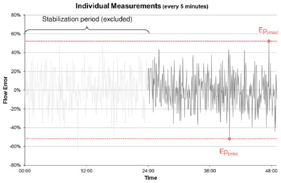
Individual flow rate measurements (5-minute intervals) after stabilization phase (n = 300 values, as recorded by the balance). Minimum and maximum deviation of single measurements are marked. As required by IEC 60601-2-24, ¹ the stabilization period is excluded.

Figure 2.

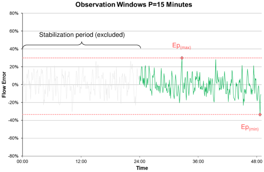
Means of flow rate errors (ie, differences between expected mean flow rate and mean of flow rate measurements) for observation windows duration P = 15 minutes after stabilization phase (n = 298 means from 3 values each). Compared to Figure 1, amplitude has decreased due to averaging several single measurements. E_p(min) and E_p(max) for P = 15 minutes are marked. Because each data point represents a mean of 3 values (ie, 15 minutes), and because the second-to-last and the last flow rate measurements cannot be the start of observation windows, the line is 2 data points shorter than in Figure 1.

Figure 3.

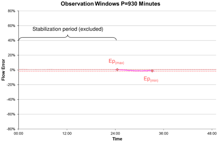
Means of flow rate errors for observation windows duration P = 930 minutes after stabilization phase (n = 115 means from 186 values each). Compared to Figure 1, amplitude has decreased due to averaging several single measurements. E_p(min) and E_p(max) for P = 930 minutes are marked. Because each data point represents a mean over 930 minutes (ie, 186 values), and because the 185th-to-last through the last flow rate measurements cannot be the start of observation windows, the line is 185 data points shorter than in Figure 1.

Figure 4.

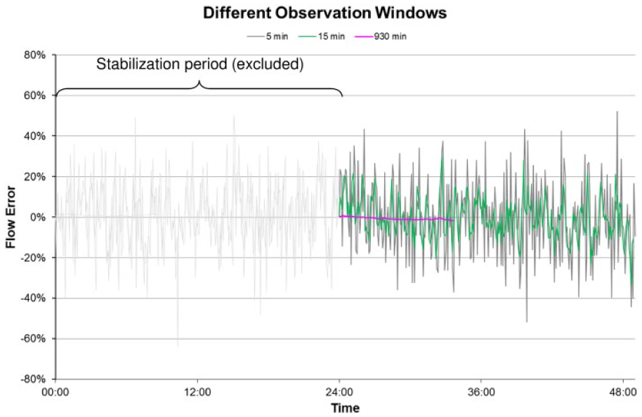
Comparison of same data in different observation windows. Single measurements (every 5 minutes, grey), 15 minutes observation windows (green) and 930 minutes observation windows (purple) are shown. As each observation window represents averaging several single measurements, amplitude and length of the lines decrease with increasing durations of the observation window.

Figure 5.

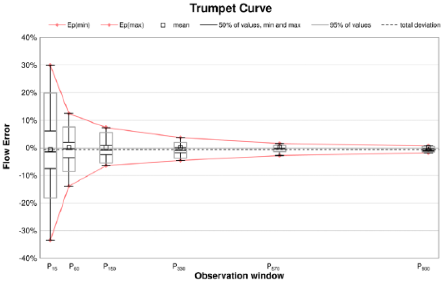
Trumpet curve as intended by IEC 60601-2-24 (E_p(min) and E_p(max) for each observation window). Additional box plots were added to highlight distribution of mean flow rate errors for each observation window. Box plots show minimum and maximum values (black antennae), interquantile range Q_25% to Q_75% (50% of all values inside black box), mean (black square), median (black line) and interquantile range Q_2.5% to Q_97.5% (95% of all values inside grey box). The box plots are based on 298, 289, 271, 235, 187, and 115 mean flow rates for P₁₅, P₆₀, P₁₅₀, P₃₃₀, P₅₇₀, and P₉₃₀, respectively.

As shown in Figures 2 and 5, the minimum flow rate for P = 15 minutes equals approximately -30% and the maximum flow rate equals approximately +30%. This means that, independent from the duration for which the pump was running, in any 15-min-long time span after a 24-hour run-in phase, basal delivery is expected to be anywhere between −30% and +30% of the flow rate set in the insulin pump. The trumpet curve (Figure 5) does not provide any information whether this was immediately after 24 hours of run-in time or, in case of the example above, around the 33-hour mark and the 49-hour mark, respectively. For some value of P between 60 and 150 minutes, both minimum and maximum flow rate are within ±10% of the set flow rate. This, again, does not mean that it takes the pump between 60 and 150 minutes to achieve ±10% deviation of the set flow rate, but rather that when averaging over time spans of at least 60 to 150 minutes, the minimum and maximum flow rate error decreases below ±10% of the set flow rate. Furthermore, the trumpet curve shows only the extreme values that do not necessarily represent general accuracy for the respective observation window. The ranges, in which 95% and 50% of values were found, as displayed in Figure 5 in boxplots, might give a more representative picture.

It may be argued that IEC 60601-2-24 does not fully appreciate the context in which insulin pumps are used. Every time a part of the insulin pump system is changed, for example, the insulin cartridge or the infusion set, the pump’s accuracy may be impacted. Current manufacturer recommendations on how often to change insulin infusion sets range from 24 hours to 72 hours. Excluding a stabilization period of 24 hours therefore seems excessive, because this amounts to 33% to 100% of the recommended wear time. In addition, patients use basal rate profiles of different rates according to their diurnal requirements rather than one constant rate. Accuracy based on a constant flow might not be meaningful anymore, especially with regard to the availability of hybrid closed-loop systems, where the basal rate is adjusted every few minutes. IEC 60601-2-24 also neglects potential effects of a mixed basal/bolus delivery, which is how insulin pumps are commonly used. From a clinical point of view, regarding dynamics and kinetics of insulin, the required observation windows could be reconsidered. Nonetheless, given that IEC 60601-2-24 is a standard of technical rather than clinical nature, the trumpet curve is an instrument to reveal the bias of basal insulin delivery.

Assessment of Insulin Dosing Accuracy beyond IEC 60601-2-24

Our proposal for the presentation of accuracy data for insulin pumps for a clinical purpose first includes all measurements over the whole experiment phase without differentiating between a stabilization period and an analysis period. A separate analysis of starting artifacts, whether caused by the pump or the test setting, may be performed. In addition, apart from showing the total flow error over the whole testing period (as percentage error from target rate), shorter time ranges should be observed. Considering the kinetics of subcutaneous insulin administration ⁶ and that insulin pumps usually enable the setting of basal rate profiles that are divided into up to 24 segments of 1 hour each, time ranges of 1 and 2 hours appear adequate. Different calculations and graphical presentations should be chosen to show on the one hand variations of accuracy and variability of the selected windows in summary, but on the other hand also accuracy in the course of time. To summarize the results and to be able to compare different insulin pumps, box plots displaying mean and median error of the individual windows of a given duration (eg, one hour) together with the 95% range (to exclude measurement artifacts that are likely to happen, eg, due to air bubbles) might be helpful. ⁵ Jahn and colleagues ⁷ presented additional analyses beyond IEC 60601-2-24 in their 2013 publication, that may facilitate comparison of different pumps’ accuracy.

Conclusion

When calculated according to IEC 60601-2-24, trumpet curves cannot show any information about required run-in times, that is, the time until the deviation from the set flow rate falls below a certain threshold. This is also due to IEC 60601-2-24 specifically excluding the first 24 hours of these experiments, because IEC 60601-2-24 requires run-in time to be addressed in a different fashion.

While IEC 60601-2-24 may not be the ideal standard regarding insulin infusion pumps, it still provides standardized requirements for testing infusion pumps. Using these standardized experimental protocols and reports as intended by IEC 60601-2-24 can make accuracy data more consistent and, subsequently, avoid confusion or misrepresentation. A standard that also defines minimum requirements to the flow rate error considering the clinical use of insulin pumps could supplement such procedural requirements.