Sage Journals: Discover world-class research

Abstract

Background:

Hyperglycemia and glucose variability in the hospital environment are associated with higher rates of complications, longer lengths of stay, and mortality. Standardized metrics are needed to assess the efficacy and safety of glucose management interventions.

Methods:

Glucometric data were collected from 2024 inpatients in a San Diego hospital between 2009 and 2011. As a complementary measure of glucose control, individual patient excursion rates were calculated using counts of distinct excursions from normal to critical glucose ranges >180 or <70 mg/dL. Prediction models for excursion rates were devised, based on patient demographic and clinical characteristics.

Results:

Patients were predominantly male (51.2%), Caucasian (86.0%), and elderly (median age 72 years). Obesity was prevalent: 32% were overweight and 33% were obese. Median length of hospitalization was 5.0 days (range, 0.8-139.4 days). Unadjusted rate of excursions >180 mg/dL was 0.456 per 24 hours. The proportion of zero excursions decreased as severity of illness decreased, but was unrelated to age. Excursion rates were slightly smaller for major and extreme severity of illness compared to mild or moderate illness severity. Excursion rates did not vary in a monotone fashion with age, although the general pattern reflected a reduction in excursion rates from the first age quartile (19 to 59) through the last age quartile (83 to 100). Using the Akaike information criterion, zero-inflated negative binomial models were identified as appropriate for analyzing glucose excursion rates.

Conclusions:

Systematic approaches to glucose reporting and management in the hospital environment offer “windows of opportunity” to improve diabetes care.

Keywords

diabetes glucometrics hospital health systems point of care testing statistical modeling

The diabetes population is expected to at least double in the next 25 years, and the cost of treating the disease will nearly triple as hospitalizations associated with diabetes continue to rise.^1,2 Hyperglycemia in the hospital environment is associated with higher rates of complications, longer lengths of stay, and higher mortality rates.^3-10 Improved glucose management has been demonstrated to reduce length of stay and improve morbidity and mortality outcomes, although reports vary on the intensity with which inpatient glucose control should be maintained.^11-16 In the current environment of increased reporting of quality outcomes, it remains critically important for health care systems to have the capacity to monitor glucose management and to set appropriate targets to minimize complications and costs. Health care systems across the nation face serious challenges when managing blood glucose levels in high-risk, hospitalized patients, and often this care is suboptimal.^17,18 Although standardized, evidence-based protocols and team management models have the potential to improve care delivery and quality outcomes in glucose management, there nevertheless remain formidable barriers to the systemwide implementation of these approaches. Moreover, a standardized metric is needed to assess and compare the efficacy and safety of these glucose management interventions.

The Society for Hospital Medicine provides guidelines for tracking glucose control in the hospital environment, but these have not been adopted consistently across health systems.^19,20 The most commonly used metrics include a day- or stay-weighted mean of glucose values using point-of-care (POC) measurements.²¹ These averages provide summaries of glucose control, but may fail to fully capture important aspects of individual patient experiences, such as hyper- or hypoglycemic events, and/or glucose variability. Indeed, glucose variability has been linked with mortality, and thus has been proposed as an important indicator of blood glucose management.²² Nevertheless, as Eslami et al²² point out, commonly used measures of variability (eg, standard deviation [SD], mean amplitude of glycemic excursions [MAGE], glycemic lability index) also have limitations, due variously to underlying asymmetric distributions of blood glucose values, sampling frequency, or severity of illness.

Scripps, one of the largest health systems in San Diego County, manages 4 hospitals on 5 campuses and 2 integrated medical groups, and is affiliated with over 1500 primary care physicians and specialists. In partnership with the Scripps Whittier Diabetes Institute (SWDI), Scripps has invested significant resources to developing a systemwide glucose management program.^23,24 In 2009, Scripps established a robust glucometric data reporting system that included the ability to determine rates of “well-managed days” (ie, days in which no more than 1 reading is outside the window of 70 to 180 mg/dL) based on hospital POC glucose testing. Adding a measure of rate to identify frequent glucose excursions can provide added information on where to target intervention efforts to provide support mechanisms and fine-tune algorithms to more rapidly bring blood glucose values into well-managed ranges. The purpose of this article is to introduce a simple metric of glucose variability: glucose excursion rate. This metric is examined using data from a 2-year observational study of glucose management conducted at Scripps. For exploratory purposes, we also examine age, gender, ethnicity, and illness severity as predictors of glucose variability.

Methods

Participants and Setting

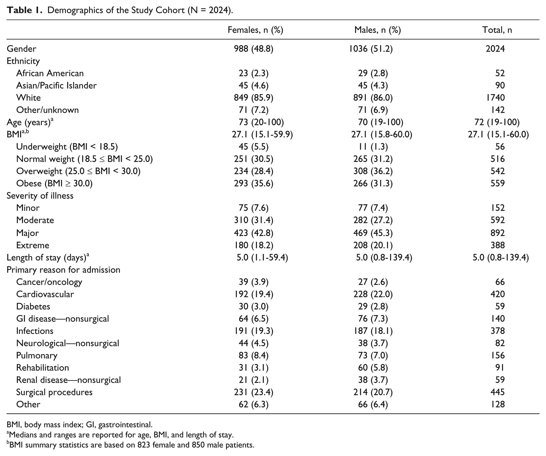
Glucometric data from Scripps Memorial Encinitas Hospital were collected from 2009 to 2011. Located in north-coastal San Diego, Scripps Memorial Encinitas has 158 beds, over 1260 employees, and 680 physicians and serves an average of 7000 unique admissions per year. The admission rate for ICD-9 codes of diabetes (250.xx) was 21% in 2010. Standard approaches to glucose management were in place during the data collection period, and no new interventions were introduced. Specifically, the target glucose range was 70 mg/dL to 180 mg/dL; excursions <70 mg/dL or >180 mg/dL triggered active intervention. Interventions included use of a standardized hypoglycemia protocol or changes to insulin regimen as directed by the attending physician to return glucose levels to the target range. All patients admitted between 2009 and 2011 and who underwent POC glucose testing over at least a 24-hour period were included in this study (N = 2024).

Data Collection

Patients’ glucose levels were monitored an average of 4 times/day in the hospital using Sure Step Hospital System, LifeScan Inc (Milipitas, CA). A Telcor interface transferred data to the Sunquest lab reporting system, and then data were sent to the electronic medical records (EMRs) to be extracted. The first 24 hours of glucose measurements were excluded from the analysis to reduce the influence of preadmission glucose control on excursion rate calculations. Predictor variables (ie, age, gender, ethnicity, severity of illness index), BMI, and primary reason for admission (both for descriptive purposes) were extracted from the Electronic Data Warehouse, which aggregates data from the EMR (GE Centricity).

Measures

Glucose Excursion Rate

Figure 1 depicts the time course of glucose levels of 2 prototypical patients monitored over the course of a 3-day hospitalization. The day-weighted mean of glucose values²¹ can be conceptualized as an area under the curve (AUC) determination, as extensively used in pharmacology: in the absence of a parametric model of glucose measurements over time, the AUC may be calculated from the trapezoid rule, which intrinsically provides the appropriate weighting of the measurements over time. Judged solely by weighted mean glucose levels, patient B evinces glucose control (weighted mean = 148.1 mg/dL), whereas patient A does not (weighted mean = 170.8 mg/dL) (see Figure 1). Note, however, that patient B’s glucose levels are widely variable, including 3 excursions > 180 mg/dL, and 1 < 70 mg/dL. If we rely on measures of variability, then the (unweighted) SD of patient A’s glucose values is 2.84, with interquartile range (IQR) 169.2 to 173.0 mg/dL, compared to patient B’s (unweighted) SD of 42.9, and IQR 124.8 to 161.8 mg/dL. This information about glucose variability is clinically relevant, but would not be captured with an exclusive reliance on mean levels. On the other hand, even these measures of spread will not necessarily reflect the frequency of excursions of glucose levels into hyper- or hypoglycemic ranges.

Figure 1.

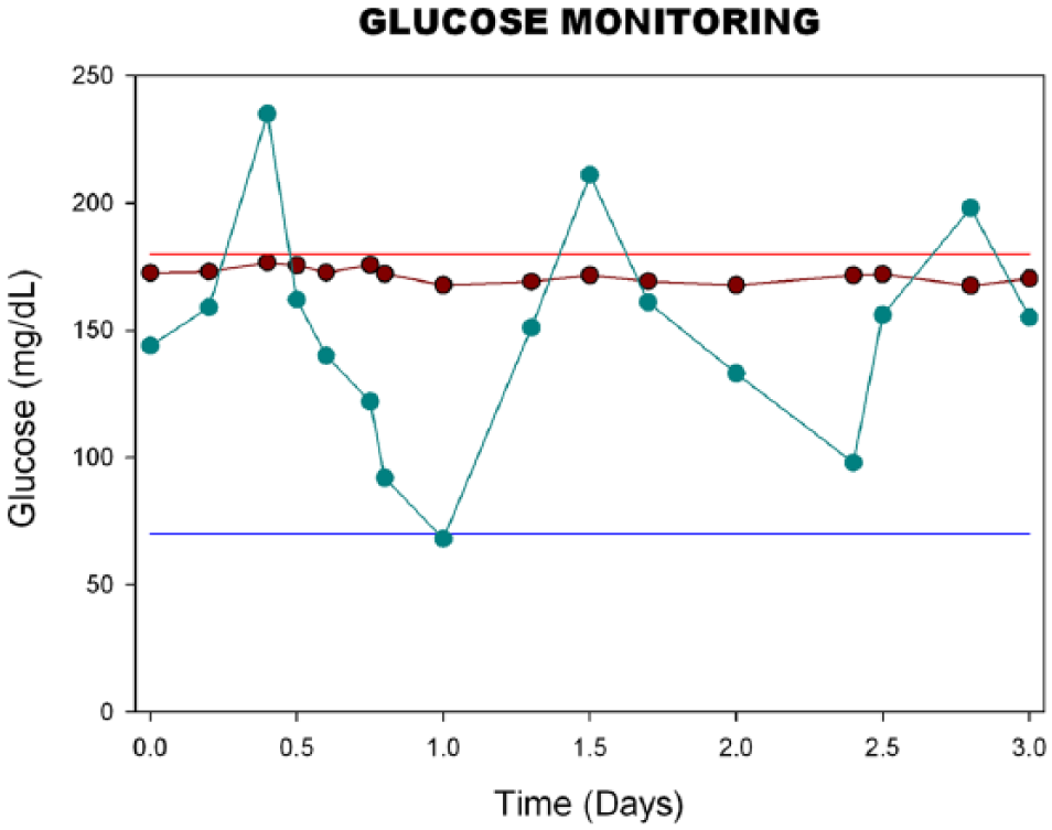
Time course of glucose levels of 2 patients, each monitored over a hospitalization period of 3 days. The solid dots indicate the times of glucose monitoring, and the patient’s glucose level at that time. Horizontal lines at reference levels 70 mg/dL (blue line) and 180 mg/dL (red line) are also depicted. Patient A (maroon line) maintained glucose levels between 70 and 180 mg/dL over the course of hospitalization, whereas patient B experienced 3 distinct excursions of glucose levels > 180 mg/dL and 1 excursion of glucose levels < 70 mg/dL over this 3-day period.

We therefore suggest counts of distinct excursions in glucose levels from the normal range to critical ranges (eg, >180 or <70 mg/dL) as a complementary measure of glucose control. Formally, an excursion is defined as a transition from the target zone to the hyper- or hypoglycemic range. Following an excursion, a subsequent reading in the hyper- or hypoglycemic zone reflects a continuation of the same excursion—that is, if 2 consecutive measurements are >180 mg/dL (or both <70 mg/dL), this is considered 1 excursion. However, once values return to the target range (70-180 mg/dL), a subsequent reading in the hyper- or hypoglycemic zone is considered a separate excursion. Note, comparing patients’ counts of excursions can be misleading if patients are monitored for dramatically different lengths of time (as might occur if lengths of hospitalization are quite disparate across patients). Hence we also extract from Figure 1 another critical source of information—that is, length of time that the patient was monitored. Numbers of excursions and length of observation time lead naturally to the determination of excursion rate. Patient A has an observed rate of zero excursions either >180 mg/dL or <70 mg/dL per 24 hours, whereas patient B has an observed rate of 1 excursion per 24 hours >180 mg/dL, and an observed excursion rate of .33 excursions per 24 hours <70 mg/dL.

Descriptive and Predictor Variables

At time of hospital admission, gender, age, ethnicity, BMI, and primary reason for admission were obtained for all patients and were coded as depicted in Table 1. Severity of illness was quantified using the 4-level all patient-refined diagnosis-related groups (APR-DRGs). The APR-DRGs expand the basic DRG structure by adding 2 sets of subclasses to each base APR-DRG. Each subclass set consists of 4 subclasses: 1 addresses patient differences relating to severity of illness and the other addresses differences in risk of mortality. Severity of illness is defined as the extent of physiologic decompensation or organ system loss of function. Risk of mortality is defined as the likelihood of dying. Statistical techniques that accommodate categorical data are appropriate when incorporating the APR-DRG severity and risk of mortality subclasses as covariates in statistical analyses. The severity of illness is assigned by the APR-DRG grouper software once the necessary data have been entered by Health Information (see http://hcup-us.ahrq.gov/db/nation/nis/grp031_aprdrg_meth_ovrview.pdf, accessed September 21, 2014).

Table 1.

Demographics of the Study Cohort (N = 2024).

	Females, n (%)	Males, n (%)	Total, n
Gender	988 (48.8)	1036 (51.2)	2024
Ethnicity
African American	23 (2.3)	29 (2.8)	52
Asian/Pacific Islander	45 (4.6)	45 (4.3)	90
White	849 (85.9)	891 (86.0)	1740
Other/unknown	71 (7.2)	71 (6.9)	142
Age (years)^a	73 (20-100)	70 (19-100)	72 (19-100)
BMI^a,b	27.1 (15.1-59.9)	27.1 (15.8-60.0)	27.1 (15.1-60.0)
Underweight (BMI < 18.5)	45 (5.5)	11 (1.3)	56
Normal weight (18.5 ≤ BMI < 25.0)	251 (30.5)	265 (31.2)	516
Overweight (25.0 ≤ BMI < 30.0)	234 (28.4)	308 (36.2)	542
Obese (BMI ≥ 30.0)	293 (35.6)	266 (31.3)	559
Severity of illness
Minor	75 (7.6)	77 (7.4)	152
Moderate	310 (31.4)	282 (27.2)	592
Major	423 (42.8)	469 (45.3)	892
Extreme	180 (18.2)	208 (20.1)	388
Length of stay (days)^a	5.0 (1.1-59.4)	5.0 (0.8-139.4)	5.0 (0.8-139.4)
Primary reason for admission
Cancer/oncology	39 (3.9)	27 (2.6)	66
Cardiovascular	192 (19.4)	228 (22.0)	420
Diabetes	30 (3.0)	29 (2.8)	59
GI disease—nonsurgical	64 (6.5)	76 (7.3)	140
Infections	191 (19.3)	187 (18.1)	378
Neurological—nonsurgical	44 (4.5)	38 (3.7)	82
Pulmonary	83 (8.4)	73 (7.0)	156
Rehabilitation	31 (3.1)	60 (5.8)	91
Renal disease—nonsurgical	21 (2.1)	38 (3.7)	59
Surgical procedures	231 (23.4)	214 (20.7)	445
Other	62 (6.3)	66 (6.4)	128

BMI, body mass index; GI, gastrointestinal.

Medians and ranges are reported for age, BMI, and length of stay.

BMI summary statistics are based on 823 female and 850 male patients.

Statistical Analyses

The comparison of glucose excursion rates can be effected by means of a straightforward statistical technique, Poisson regression. Poisson regression is similar to linear regression, except that the dependent variable is a count (here, number of excursions) rather than a continuous variable, and there is a quantity called an “offset” (in our setting, the natural logarithm of the length of observation time) that is incorporated into the regression scheme, so as to adjust the counts for differing lengths of observation. As with linear regression, Poisson regression easily incorporates both continuous variables (eg, age) and categorical variables (eg, ethnicity, gender, severity of illness) as predictors.

Poisson regression is naturally invoked with count data as the dependent variable. Nevertheless, generalizations of Poisson regression exist, if counts exhibit “extra-Poisson variability.” Such would exist, for example, if individual counts are Poisson-distributed, but the Poisson parameter varies across individuals according to a gamma distribution. The resulting counts have a negative binomial distribution, and, accordingly, negative binomial regression would be utilized for subsequent analyses assessing how counts vary with potential predictor variables.

In settings where there are an excess of zero counts, 2 further generalizations of regression with count outcomes are available, namely, zero-inflated Poisson regression and zero-inflated negative binomial inflation.

For each fitted model, we determined log likelihoods and used the Akaike information criterion (AIC)²⁵ as a rigorous model selection criterion. Likelihoods [and log likelihoods] are numerically maximized during model fitting, whereas the AIC is a measure of information loss with a given model. Hence preferred models have larger likelihoods, or minimal AIC values. To aid further with model selection, we also calculated Vuong statistics²⁶ for assessing whether the zero-inflated models were significant improvements over their non-zero-inflated counterparts. All models were fitted in Stata version 12 (StataCorp, College Station, TX).

We fit 4 regression models to the individual patient excursion counts: Poisson regression, negative binomial regression, zero-inflated Poisson regression, and zero-inflated negative binomial regression. Our putative predictors (main effects) were gender, ethnicity, illness severity, and age, both for the counts and for the inflation variables in the cases of the zero-inflated models. We also incorporated an offset variable to accommodate variance in length of stay. Optimal model selection was determined by AIC measures as explained above, supplemented with Vuong statistics.

Results

Descriptives

Descriptive statistics for the 2024 patients included in this study are shown in Table 1. Patients were predominantly male (51.2%), Caucasian (86.0%), and elderly (median age 72, range 19-100 years). Obesity was prevalent: about 32% of patients were overweight (BMI = 25.0-29.9), and 33% of patients were obese (BMI ≥ 30). Median length of hospitalization was 5.0 days (range, 0.8-139.4 days).

Glucose Excursion Rates

Across the 2024 patients, the unadjusted (crude) rate of excursions <70 mg/dL was 0.043/24 hours (430 excursions / 10 044.96 patient-days), and the unadjusted rates of excursions > 180 mg/dL was 0.456/24 hours (4583 excursions / 10 044.96 patient-days). Due to the relative paucity of excursions <70 mg/dL, we will henceforth focus on excursions >180 mg/dL, and investigate suitable models for these excursions.

The crude rates obscure significant patient-to-patient variability in individual excursion rates. In Figure 2 we present a histogram of individual excursion rates for all 2024 patients. From this figure, it should be immediately apparent that there are an excess of zero rates in our cohort, the implication being that zero-inflated models are likely to be more appropriate than their non-zero-inflated counterparts.

Figure 2.

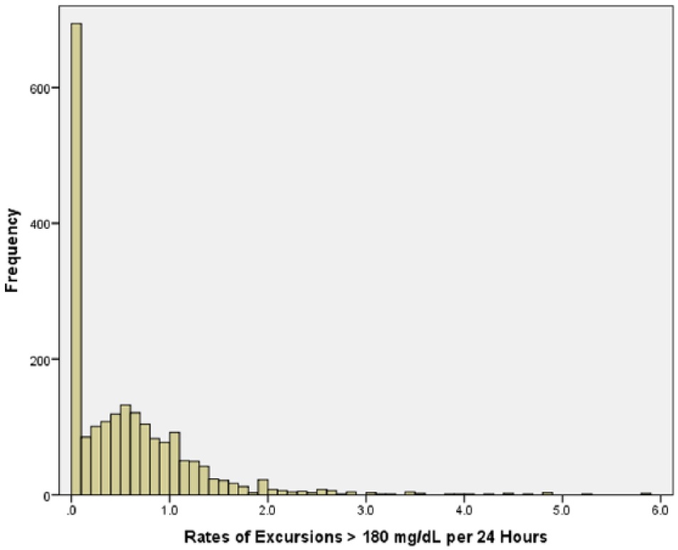
Histogram of individual excursion rates (# excursions > 180 mg/dL per 24 hours) for the entire cohort of 2024 patients. There were 677 patients (33.4%) with no excursions, and 1347 (66.6%) with 1 or more excursions.

Prediction Models

We present summary statistics from these 4 models in Table 2. In general, models with larger log likelihoods (smaller negative log likelihoods) and smaller AICs are preferable. In addition, we calculated Vuong tests for comparing the Poisson model with the zero-inflated Poisson model (z = 5.78, P < .0001), and for comparing the negative binomial model with the zero-inflated negative binomial model (z = 4.12, P < .0001). From these statistics as well as Figure 2, the zero-inflate negative binomial model best fit the clinical data; hence we chose to limit consideration to this model, and examined parameter estimation within this model more closely.

Table 2.

Summary Statistics for Model Selection Among 4 Different Models.

Model	Log likelihood	df	AIC
Poisson	−3892.9	9	7803.8
Negative binomial	−3545.6	10	7111.1
Zero-inflated Poisson	−3666.0	16	7368.0
Zero-inflated negative binomial	−3493.3	18	7024.7

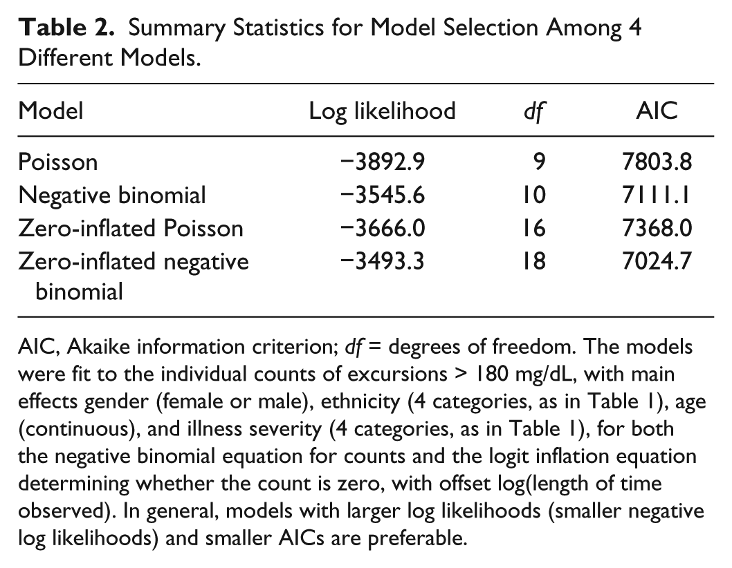
AIC, Akaike information criterion; df = degrees of freedom. The models were fit to the individual counts of excursions > 180 mg/dL, with main effects gender (female or male), ethnicity (4 categories, as in Table 1), age (continuous), and illness severity (4 categories, as in Table 1), for both the negative binomial equation for counts and the logit inflation equation determining whether the count is zero, with offset log(length of time observed). In general, models with larger log likelihoods (smaller negative log likelihoods) and smaller AICs are preferable.

In the statistical appendix, we present details concerning our final zero-inflated negative binomial model: of the initial variables we had entered into consideration, we found that only severity of illness was a significant predictor of inflation (excess zeros), and both age and severity of illness were significant predictors of excursion rates. To illustrate the associations of age and severity of illness with excursions, we present histograms of excursion rates in Figures 3 and 4, and summary statistics in Tables 3 and 4. With regard to excess zeros, note the monotone trend in Table 3: as severity of illness increases, the proportion of zero excursions decreases. In contrast, the proportion of zero excursions appears unrelated to age (Table 4). Excursion rates evince a different pattern: excursion rates do not increase with increasing severity of illness, but tend to be slightly smaller for major and extreme severity of illness compared to mild or moderate illness severity. Nor do excursion rates vary in a monotone fashion with age, although the general pattern is a reduction in excursion rates from the first age quartile (19 to 59) through the last age quartile (83 to 100).

Figure 3.

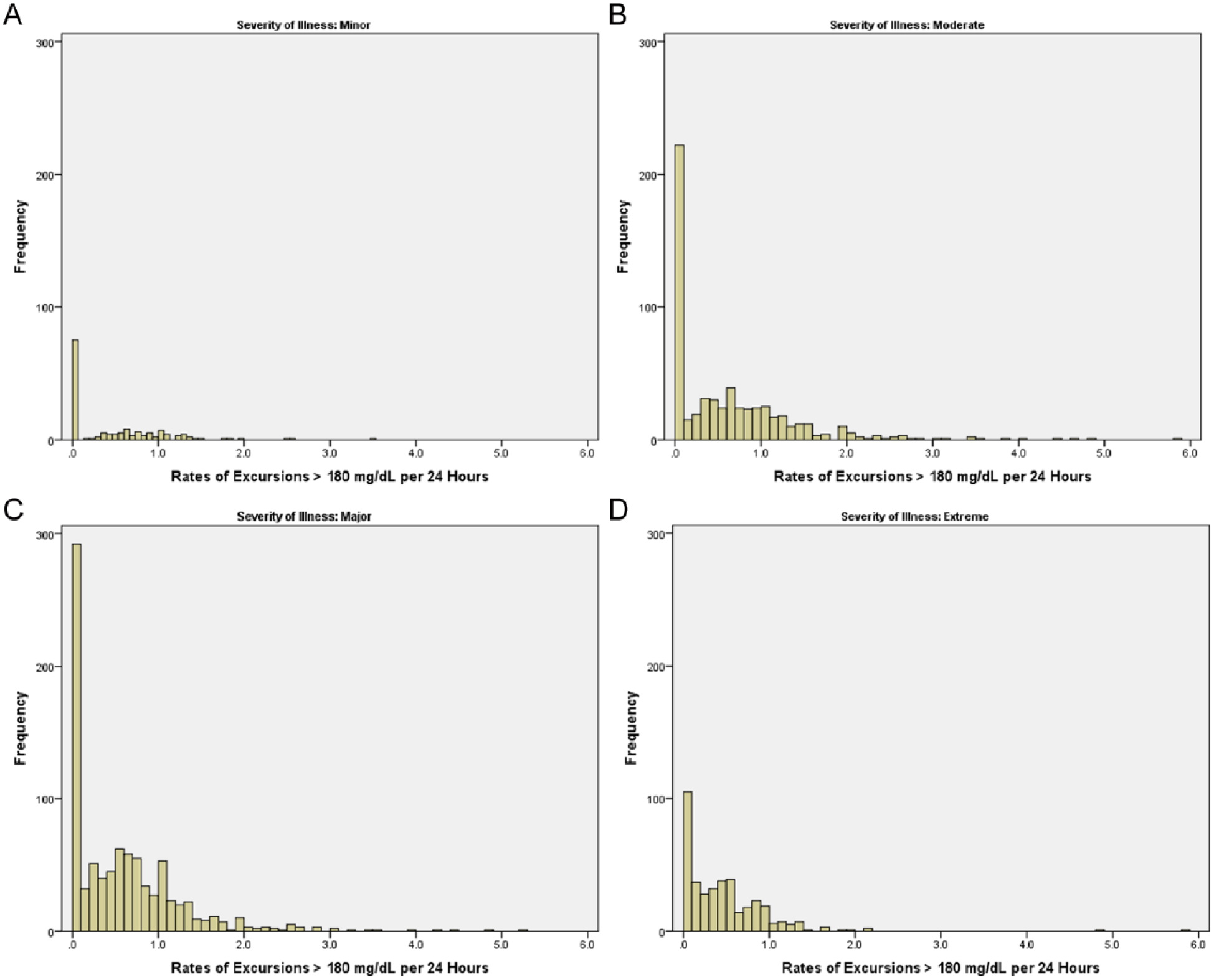
Histograms of individual excursion rates (# excursions > 180 mg/dL per 24 hours) for the entire cohort of 2024 patients, grouped by severity of illness. (A) Mild severity of illness, n = 152. There were 75 patients (49.3%) with no excursions, and 77 (50.7%) with 1 or more excursions. (B) Moderate severity of illness, n = 592. There were 220 patients (37.2%) with no excursions, and 372 (62.8%) with 1 or more excursions. (C) Major severity of illness, n = 892. There were 285 patients (32.0%) with no excursions, and 607 (68.0%) with 1 or more excursions. (D) Extreme severity of illness, n = 388. There were 97 patients (25.0%) with no excursions, and 291 (75.0%) with 1 or more excursions.

Figure 4.

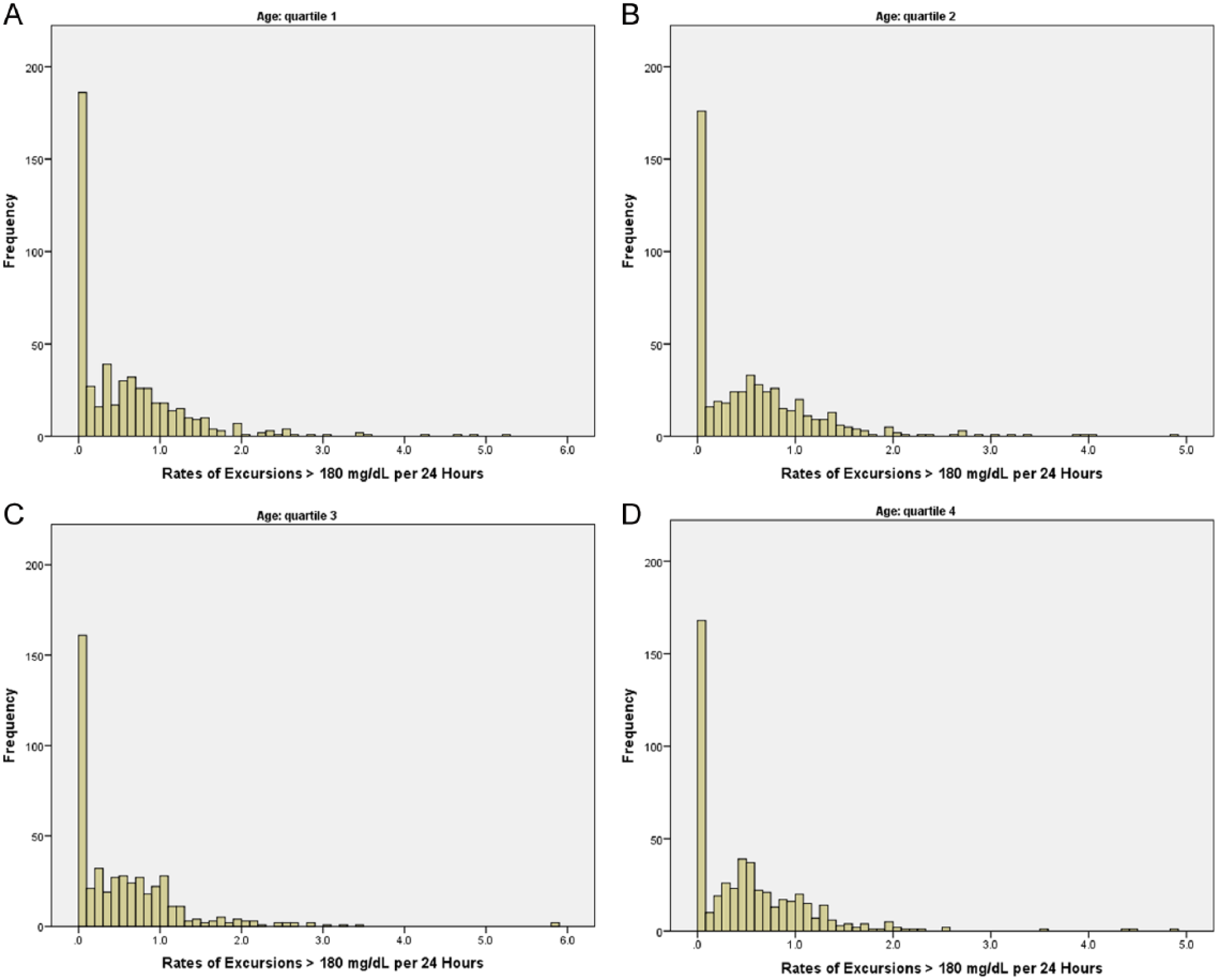
Histograms of individual excursion rates (# excursions > 180 mg/dL per 24 hours) for the entire cohort of 2024 patients, grouped by age quartiles. (A) Ages 19 to 59, n = 528. There were 180 patients (34.1%) with no excursions, and 348 (65.9%) with 1 or more excursions. (B) Ages 60 to 72, n = 520. There were 172 patients (33.1%) with no excursions, and 348 (66.9%) with 1 or more excursions. (C) Ages 73 to 82, n = 472. There were 159 patients (33.7%) with no excursions, and 313 (66.3%) with 1 or more excursions. (D) Ages 83 to 100, n = 504. There were 166 patients (32.9%) with no excursions, and 338 (67.1%) with 1 or more excursions.

Table 3.

Rates of Excursions > 180 mg/dL per 24 Hours, by Severity of Illness Classification.

Severity of illness	No excursions, n (%)	Excursions, n (%)	Excursion rate (mean, SD)
Mild (n = 152)	75 (49.3)	77 (50.7)	0.913, 0.551
Moderate (n = 592)	220 (37.2)	372 (62.8)	0.991, 0.776
Major (n = 892)	285 (32.0)	607 (68.0)	0.866, 0.662
Extreme (n = 388)	97 (25.0)	291 (75.0)	0.614, 0.551

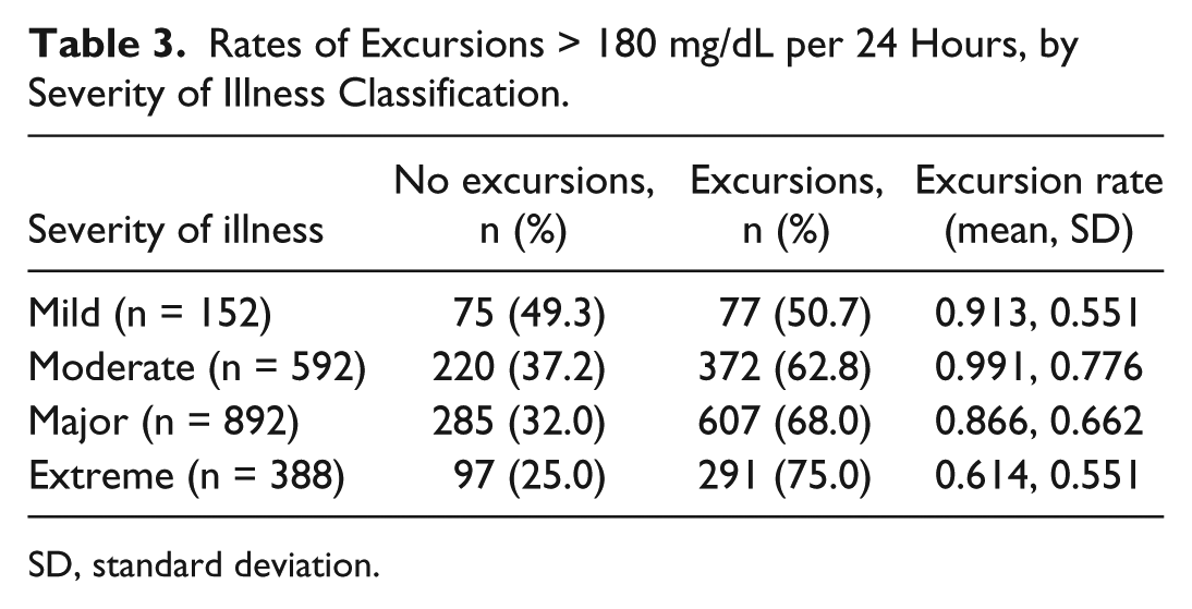
SD, standard deviation.

Table 4.

Rates of Excursions > 180 mg/dL per 24 Hours, by Age Quartiles.

Age	No excursions, n (%)	Excursions, n (%)	Excursion rate (mean, SD)
19 to 59 (n = 528)	180 (34.1)	348 (65.9)	0.895, 0.738
60 to 72 (n = 520)	172 (33.1)	348 (66.9)	0.848, 0.660
73 to 82 (n = 472)	159 (33.7)	313 (66.3)	0.856, 0.715
83 to 100 (n = 504)	166 (32.9)	338 (67.1)	0.794, 0.605

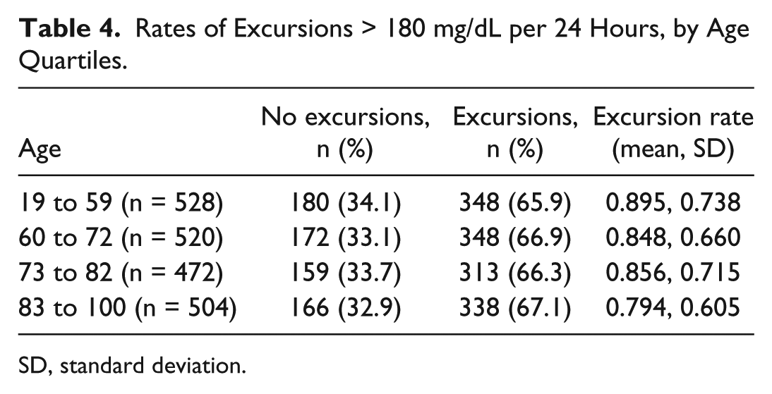
SD, standard deviation.

Discussion

Despite an increased awareness of the importance of effective inpatient diabetes management, little is known about glucose control in hospitals. Furthermore, many hospitals across the nation have developed glucose management protocols, yet are unable to determine their effectiveness. This article examined “glucose excursion rate” as a metric of glucose variability that might be used systematically and in a complementary fashion with day-weighted glucose means across patients and health systems to evaluate interventions established to improve glucose management. In contrast to a day- or stay-weighted mean, an excursion indicates an event that may trigger an intervention (see Figure 1). Some literature has indicated that acute fluctuations of glucose around a mean value activates the oxidative stress cascade and may contribute to longer-term deleterious effects.^27-33 Excursion rates also offer advantages over existing variability indices (eg, MAGE, IQR, SD, glycemic lability), in that the latter do not capture the frequency of unique excursions into hyper- or hypoglycemic ranges. Previous research also indicates that current glucose variability indicators are sensitive to the asymmetric distribution of blood glucose values and sampling frequency, and/or may merely reflect illness severity.²² Thus, utilizing a metric that better captures glucose variability may allow more consistent analysis of patient outcomes across hospitals and health systems.

Findings suggested that zero-inflated negative binomial models are appropriate for regression analyses of glucose excursion rates. An immediate implication of this model is that there is a subset of patients who are not at risk for excursions during hospitalization; the other patients evince heterogeneity in excursion rates, overdispersed relative to a Poisson distribution of excursions. Exploratory analyses of these models indicated that severity of illness was a significant predictor of inflation (“zero excursion”); as expected, patients with higher severity of illness were more likely to exhibit 1 or more excursion(s) than those with relatively lower illness severity. However, the story is less clear among the subset of patients with 1 or more excursion(s). Contrary to predictions, in this group, the rate of excursions decreased with increasing age and increasing illness severity. Associations of sex and ethnicity with excursion rate were not statistically significant. Although the direction of these findings complicates interpretation, it is possible that patients admitted with type 1 diabetes and diabetic ketoacidosis were younger and exhibited higher excursion rates. Another potential explanation is that, on average, as age increases diabetes becomes easier to manage. For illness severity, it is possible that the more severe patients will be monitored more closely in the hospital, thus leading to lower excursion rates. Nonetheless, further research is needed to better understand these unexpected findings.

Several limitations should be considered in the interpretation of these findings. First, due to the observational nature of this study, blood glucose monitoring was not necessarily comprehensive, and we may have missed individual patient excursions. Future studies should consider more systematic daily monitoring schemes, for example through the use of continuous glucose monitors. Next, this analysis was based on 1 hospital sample and examined a single metric of glucose variability. Moving forward, research should examine the utility of the glucose excursion rate metric in other (diverse) health care systems for cross-validation purposes. Studies that investigate the additive value of glucose excursion rates over and above the information conveyed by patient-day-weighted means, and/or compare the proposed glucose excursion rate metric against other measures of glucose variability would also represent valuable additions to the literature. Additional predictors of glucose variability (eg, diabetes diagnosis) also warrant consideration as well as evaluating the hospital and longer-term outcomes related to the glucose excursion rates. Identifying an association between glucose excursion rates and clinical outcomes was beyond the scope of this article but should be included in subsequent studies. Moreover, investigating these research questions across multiple inpatient sites and validating this metric separately in type 1 and type 2 diabetes would add value to the findings.

Conclusions

The overwhelming majority of hospitalizations for patients with diabetes occur for treatment of comorbid conditions, and frequently, abnormal glucose trends are missed or masked during the hospitalization. Patients with newly recognized hyperglycemia, poorly controlled glucose levels, and/or or high glucose variability have a higher rate of mortality during their hospitalization.³ Although further research is needed, available findings suggest that minimizing glucose variability may have positive implications for micro- and, to some extent, macrovascular diabetic complications (for a review, see Krishna et al³⁴). Using glucometrics reports with complementary measures will identify these patients more accurately and potentially flag them as higher risk patients requiring more intensive follow up. The proposed metric, glucose excursion rate, depicts the frequency of hypo- or hyperglycemic events—that is, an aspect of blood glucose management that is not captured by current indicators of average glucose or glucose variability. This metric may better inform our care, but more research is needed before it can be used to leverage improvements in clinical care. Having a glucose management team and protocols in place to lower glucose levels during the hospitalization and, possibly even more important, educating the patient on the fact that he or she has diabetes and must follow up the care of his or her diabetes postdischarge are support systems that can be added as resources for the identified higher risk patients and may have an impact on the morbidity and mortality outcomes of the associated conditions. Systematic approaches to glucose reporting and management in the hospital environment offer “windows of opportunity” to improve diabetes care when patients with diabetes are hospitalized for other conditions, to improve diabetes self-care instruction before discharge, and to address important knowledge deficits in the patient and his or her family.

Footnotes

Statistical Appendix

In this appendix, we describe our model fitting in Stata 12. We begin with the command executed in Stata for fitting our summary zero-inflated negative binomial regression model:

.zinb CntExcGT180 c.Age##i.SevIllness, inflate(i.SevIllness, offset(day_offset)) offset(day_offset) irr vuong zip allbaselevels

Let us parse this command, as follows.

Our data set contains variables

With zinb, we are requesting a zero-inflated negative binomial regression model for counts of excursions > 180 (dependent variable) with an offset, the day_offset variable; effectively, we are analyzing rates of excursions over 24 hours as our dependent variable.

The term c.Age##i.SevIllness in the command is denoting a model for the rates with main effects Age (continuous), Severity of Illness (categorical variable, 4 levels), as well as interaction terms between Age and the levels of SevIllness.

The term inflate(i.SevIllness, offset (day_offset)) is specifying a logit model for the inflated zeros, with 1 main effect (severity of Illness, categorical) and the offset day_offset.

We are also requesting rate ratios with irr (incidence rate ratio, in Stata’s terminology). In this regard, the rate ratios are determined relative to the base levels of the factors. Other options include zip, the likelihood ratio test for comparing the zero-inflated Poisson with the zero-inflated negative binomial, and vuong, the Vuong statistic for comparing the zero-inflated negative binomial model with the standard negative binomial model (no inflation).

Here is some Stata output.

Initially, Stata presents a model summary, as follows:

Zero-inflated negative binomial regression

Number of obs = 2024

Nonzero obs = 1347

Zero obs = 677

Inflation model = logit

LR chi2(7) = 42.82

Log likelihood = -3488.156

Prob > chi2 = 0.0000

Stata has fit a zero-inflated negative binomial regression model with 2024 observations (patients), of whom 677 had no excursions > 180 mg/dL, and 1347 had 1 or more excursions. The inflation model (model for the excess zeroes) is a logit model for predicting whether a patient will be a zero (no excursions) or not. The log likelihood for the fitted model is −3488.156, and the log likelihood for the null model (no predictors) is −3509.564 (not shown); the likelihood ratio chi-square statistic for assessing whether the fitted model is an improvement over the null model is −2 * (–3509.564 – (–3488.156)) = 42.82 with 7 degrees of freedom; the P value associated with this likelihood ratio test is < .0001. The fitted model represents a significant improvement over the null model.

Next, Stata outputs parameter estimates, as follows:

The top part of this table relates to the full model for rates of excursions > 180 mg/dL. IRR denotes the incidence rate ratio, as before. Stata is presenting the rate ratios (IRR), the standard errors of these estimates, the corresponding z statistics (IRR/st.err.), the 2-sided P values attending these z statistics (denoted P>|z|), and 95% confidence intervals for the IRR coefficients.

The IRR corresponding to Age is .98, indicating a decrease in excursion rates with increasing age: for each unit (1 year) increase in age, the rate of excursions is estimated as .98 the previous year’s rate.

Recall that Sevillness is treated as a categorical variable in this model, with mild severity of illness ( category 1) as the baseline, followed by moderate (category 2), major (category 3), or extreme (category 4). In the full model, the estimated rate of excursions > 180 mg/dL for moderate severity is .74 the baseline rate, .38 of the baseline rate for major severity, and .19 the baseline rate for extreme severity.

We have also included interaction terms, SevIllness#Age, in the regression model, as these allow fine-tuning of rate estimates.

The constant term, denoted cons, is the predicted rate of excursions if all of the other predictor variables in the model are evaluated at 0.

The second part of this table, with the heading inflate, refers to the logistic model predicting whether a patient is an excess zero. Here, there is only 1 predictor, severity of illness, and the coefficients represent factor changes in the log odds of being an excessive zero (no excursions). That is, the log odds of being an excessive zero would decrease by 1.42 for moderate severity relative to mild severity (baseline), by 1.01 for major severity relative to baseline, and by 2.19 for extreme severity relative to baseline. Informally, a patient is more likely to have excursions as severity of illness increases.

At the bottom of the output, the likelihood ratio test of alpha = 0 is assessing whether there is a significant improvement of fit with a zero-inflated negative binomial model compared to a zero-inflated Poisson model (alpha = 0). The likelihood ratio test is a chi-square statistic, with 1 degree of freedom. Clearly, the negative binomial represents a significant improvement over the Poisson.

Also at the bottom, the Vuong test suggests that the zero-inflated negative binomial model is a significant improvement over a standard (non-zero-inflated) negative binomial model.

Acknowledgements

We thank the reviewers for their thoughtful comments, which led to material improvements in the manuscript.

Abbreviations

AIC, Akaike information criterion; APR-DRGs, all patient-refined diagnosis-related groups; AUC, area under the curve; DF, degrees of freedom; EMR, electronic medical record; IQR, interquartile range; MAGE, mean amplitude of glycemic excursions; POC, point of care; SD, standard deviation; SWDI, Scripps Whittier Diabetes Institute.

Declaration of Conflicting Interests

The author(s) declared no potential conflicts of interest with respect to the research, authorship, and/or publication of this article.

Funding

The author(s) disclosed receipt of the following financial support for the research, authorship, and/or publication of this article: Support for this work came from Scripps Health, an educational grant from Sanofi, and a research grant from Novo Nordisk.

References

Huang

Basu

O’Grady

Capretta

. Projecting the future diabetes population size and related costs for the U.S. Diabetes Care. 2009;32:2225-2229.

Centers for Disease Control and Prevention. Number (in thousands) of hospital discharges with diabetes as any-listed diagnosis, United States, 1988-2009. http://www.cdc.gov/diabetes/statistics/dmany/fig1.htm.

Umpierrez

Isaacs

Bazargan

You

Thaler

Kitabchi

. Hyperglycemia: an independent marker of in-hospital mortality in patients with undiagnosed diabetes. J Clin Endocrinol Metab. 2002;87:978-982.

Falciglia

Freyberg

Almenoff

D’Alessio

Render

. Hyperglycemia-related mortality in critically ill patients varies with admission diagnosis. Crit Care Med. 2009;37(12):3001-3009.

Krinsley

. Association between hyperglycemia and increased hospital mortality in a heterogeneous population of critically ill patients. Mayo Clin Proc. 2003;78(12):1471-1478.

Norhammar

Tenerz

Nilsson

. Glucose metabolism in patients with acute myocardial infarction and no previous diagnosis of diabetes mellitus: a prospective study. Lancet. 2002;359:2140-2144.

Matz

Keresztes

Tatschl

. Disorders of glucose metabolism in acute stroke patients: an underrecognized problem. Diabetes Care. 2006;29:792-797.

Capes

Hunt

Malmberg

Gerstein

. Stress hyperglycaemia and increased risk of death after myocardial infarction in patients with and without diabetes: a systematic overview. Lancet. 2000;355:773-778.

Meier

Deifuss

Klamann

Launhardt

Schmiegel

Nauck

. Plasma glucose at hospital admission and previous metabolic control determine myocardial infarct size and survival in patients with and without type 2 diabetes: the Langendreer Myocardial Infarction and Blood Glucose in Diabetic Patients Assessment (LAMBDA). Diabetes Care. 2005;28:2551-2553.

10.

McAlister

Majumdar

Blitz

Rowe

Romney

Marrie

. The relation between hyperglycemia and outcomes in 2,471 patients admitted to the hospital with community-acquired pneumonia. Diabetes Care. 2005;28:810-815.

11.

Van den Berghe

Wouters

Weekers

. Intensive insulin therapy in critically ill patients. N Engl J Med. 2001;345(19):1359-1367.

12.

Umpierrez

Hellman

Korytkowski

. Management of hyperglycemia in hospitalized patients in non-critical care setting: an Endocrine Society clinical practice guideline. J Clin Endocrinol Metab. 2012;97:16-38.

13.

Umpierrez

Smiley

Jacobs

. Randomized study of basal-bolus insulin therapy in the inpatient management of patients with type 2 diabetes undergoing general surgery (RABBIT 2 surgery). Diabetes Care. 2011; 34:256.

14.

Griesdale

de Souza

van Dam

. Intensive insulin therapy and mortality among critically ill patients: a meta-analysis including NICE-SUGAR study data. CMAJ. 2009;180(8):821-827.

15.

Wiener

Larson

. Benefits and risks of tight glucose control in critically ill adults: a meta-analysis. JAMA. 2008;300(8):933-944.

16.

Kansagara

Freeman

Wolf

Helfand

. Intensive insulin therapy in hospitalized patients: a systematic review. Ann Intern Med. 2011;154(4):268-282.

17.

Cook

Kongable

Potter

Abad

Leija

Anderson

. Inpatient glucose control: a glycemic survey of 126 U.S. hospitals. J Hosp Med. 2009;4:E7-E14.

18.

Swanson

Potter

Kongable

Cook

. Update on inpatient glycemic control in hospitals in the United States. Endocr Pract. 2011;17(6):853-861.

19.

Society of Hospital Medicine. http://www.hospitalmedicine.org/ResourceRoomRedesign/html/06Track_Perf/02_Introducing_Gluco.cfm. Accessed May 15, 2014.

20.

Schnipper

Magee

Larsen

. Society of Hospital Medicine Glycemic Control Task Force summary: practical recommendations for assessing the impact of glycemic control efforts. J Hosp Med. 2008;3(suppl 5):66-75.

21.

Goldberg

Bozzo

Thomas

. “Glucometrics”—assessing the quality of inpatient glucose management. Diabetes Technol Therap. 2006;8:5;560-569.

22.

Eslami

Taherzadeh

Schultz

Abu-Hanna

. Glucose variability measures and their effect on mortality: a systematic review. Intensive Care Med. 2011;37:583-593.

23.

Morrisey

Decker

Finger

. Implementation of a standardized glucose management program across a large hospital system-1 year results. Paper presented at the ADA 72nd Scientific Sessions; 2012; Philadelphia, PA.

24.

Decker

Morrisey

Finger

Deutzer

Philis-Tsimikas

. Standardized curriculum and education pathway supports the implementation of systemwide hospital glucose management. Paper presented at the ADA 72nd Scientific Sessions; 2012; Philadelphia, PA.

25.

Akaike

. A new look at the statistical model identification. IEEE Trans Automatic Control. 1974;19:716-723.

26.

Vuong

. Likelihood ratio tests for model selection and non-nested hypotheses. Econometrica. 1989;57:307-334.

27.

Monnier

Mas

Ginet

. Activation of oxidative stress by acute glucose fluctuations compared with sustained chronic hyperglycemia in patients with type 2 diabetes. JAMA. 2006;295:1681-1687.

28.

Esposito

Nappo

Marfella

. Inflammatory cytokine concentrations are acutely increased by hyperglycemia in humans: role of oxidative stress. Circulation. 2002;106:2067-2072.

29.

Egi

Bellomo

Stachowski

French

Hart

. Variability of blood glucose concentration and short-term mortality in critically ill patients. Anesthesiology. 2006;105:244-252.

30.

Krinsley

. Glycemic variability: a strong independent predictor of mortality in critically ill patients. Crit Care Med. 2008;36:3008-3013.

31.

Krinsley

. Glycemic variability and mortality in critically ill patients: the impact of diabetes. J Diabetes Sci Technol. 2009;3:1292-1301.

32.

Dossett

Cao

Mowery

Dortch

Morris

Jr May

. Blood glucose variability is associated with mortality in the surgical intensive care unit. Am Surg. 2008;74:679-685; discussion 685.

33.

Lipska

Venkitachalam

Gosch

. Glucose variability and mortality in patients hospitalized with acute myocardial infarction. Circ Cardiovasc Qual Outcomes. 2012;5:550-557.

34.

Krishna

Kota

Modi

. Glycemic variability: clinical implications. Ind J Endocrinol Metab. 2013;17(4):611-619.

Novel Approach to Inpatient Glucometric Monitoring and Variability in a Community Hospital Setting

Abstract

Background:

Methods:

Results:

Conclusions:

Keywords

Methods

Participants and Setting

Data Collection

Measures

Glucose Excursion Rate

Descriptive and Predictor Variables

Statistical Analyses

Results

Descriptives

Glucose Excursion Rates

Prediction Models

Discussion

Conclusions

Footnotes

Statistical Appendix

Acknowledgements

Abbreviations

Declaration of Conflicting Interests

Funding

References