
Abstract
Background:
One way of constructing a control algorithm for an artificial pancreas is to identify a model capable of predicting plasma glucose (PG) from interstitial glucose (IG) observations. Stochastic differential equations (SDEs) make it possible to account both for the unknown influence of the continuous glucose monitor (CGM) and for unknown physiological influences. Combined with prior knowledge about the measurement devices, this approach can be used to obtain a robust predictive model.
Method:
A stochastic-differential-equation-based gray box (SDE-GB) model is formulated on the basis of an identifiable physiological model of the glucoregulatory system for type 1 diabetes mellitus (T1DM) patients. A Bayesian method is used to estimate robust parameters from clinical data. The models are then used to predict PG from IG observations from 2 separate study occasions on the same patient.
Results:
First, all statistically significant diffusion terms of the model are identified using likelihood ratio tests, yielding inclusion of
Conclusions:
This study shows that SDE-GBs and a Bayesian method can be used to identify a reliable model for prediction of PG using IG observations obtained with a CGM. The model could eventually be used in an artificial pancreas.
Keywords
The use of continuous glucose monitors (CGMs) on patients with type 1 diabetes mellitus (T1DM) has a positive effect on glycemic control.1-5 The advantages of continuous glucose monitoring are many, but there are also several well-documented problems.6-8 These include time delay between plasma glucose (PG) and interstitial glucose (IG),3-5 the drift of sensor sensitivity, 9 and vulnerability to calibrations during rapidly increasing or decreasing glucose levels.10,11 For optimal use of CGMs in the management of T1DM, for example, for closed-loop control, it is necessary to know the relationship between PG and IG. 12 Due to the well-known issues with the sensor, the main challenge related to automatic control of the glucose is to predict PG from IG observations measured by a CGM. To do this, the dynamical relation between the PG and IG levels needs to be well described.
Modeling glucose dynamics using observations from CGMs is challenging. As described by Facchinetti et al., three of the major problems are (1) PG observations have to be collected parallel with IG observations, (2) a precise model for PG-IG dynamics is needed, and (3) sensor errors should be modeled as stochastic processes. 13
When using real-life data obtained with a CGM, the autocorrelation of data becomes an issue, requiring specific modeling techniques. This is discussed in this article. As the observations are closely sampled (e.g., 5-minute sample rate), interdependence between data points or autocorrelation is present.14-16 Several approaches to overcome sensor issues, including autocorrelation, have been investigated.17-19 Data-driven autoregressive models have been used by Reifman et al. 16 Chase et al. modeled sensor errors using Gaussian processes. 20 Breton and Kovatchev used a non-Gaussian Johnson distribution and autoregressive (AR(1) processes). 21 One suggestion by Guerra et al. is to use deconvolution-based enhancement algorithms that, in real time, improve CGM accuracy. 22
In this study we use stochastic-differential-equation-based gray-box (SDE-GB) models and a Bayesian method to address all 3 issues described by Facchinetti et al.
When investigating the glucose-insulin dynamics (e.g., in closed-loop studies), patients receive inputs to excitate glucose values, such as meals, giving a positive excitation and insulin, giving a negative excitation. This article accommodates the need for an understanding of the dynamics with no external positive excitation. The negative excitation is provided by a continuous subcutaneous insulin infusion (CSII).
Glucose-insulin dynamics are a part of the complex, partly unknown fuel metabolism. 23 Stochastic behavior should therefore be considered in the modeling. One way of doing this is to apply SDE-GB models. Such models are established using a combination of physiological knowledge and statistical information from data. In general a SDE-GB model can be written as,
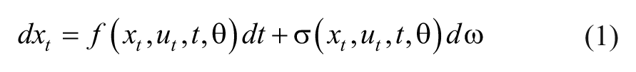
where the states are described by the vector
The advantage of using SDE-GB models as compared to ordinary differential-equations-based models, is that noise is included in the state equations in terms of
Methods
The data used in this study originate from an overnight closed-loop study, conducted as a part of the DIACON project. 34 The patient was studied on 2 overnight hospital admissions from 17:30 to 07:00. At 18:00, an evening meal was served. The size of the meal was determined by patient weight (1 g carbohydrate/kg body weight) and was identical on the 2 study nights. The bolus calculator in the patient’s own insulin pump was used to determine the size of the meal bolus. At 22:00 the study initiated. No further food or insulin boluses were given. 34 PG and plasma insulin were sampled every 30 minutes. PG was analyzed using YSI2300 STAT Plus (Yellow Springs Instruments, Yellow Springs, OH). Every 5 minutes a subcutaneous glucose value was obtained using a Dexcom SEVEN PLUS (Dexcom, San Diego, CA) CGM. Insulin Aspart (Novorapid, Novo Nordisk, Bagsværd, Denmark) was administered using a Paradigm Veo (Medtronic, Northridge, CA) insulin pump. Patients were euglycemic (PG level 70-144 mg/dl) at study start. It is assumed that an evening meal given 4 hours before study start does not influence the glucose dynamics. For this study, data from on 1 patient on 2 independent nights at least 2 weeks apart were used. The first data set, Data1, originates from a closed-loop study night, and the second data set, Data2, originates from an open-loop study night.
The Initial Model
The MVP model was used as the basis for formulating the SDE-GB model. In essence, the model is based on the Bergman minimal model.35,36 Fisher modified the model, replacing insulin secretion with insulin infusion. 37 In this study, we focus on the kinetics and dynamics when patients are at rest. This reduces the model to the 5 equations below describing glucose-insulin dynamics with no meal input.
The insulin dynamics are described by,
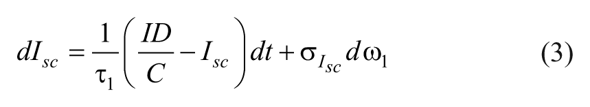
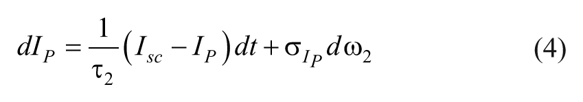
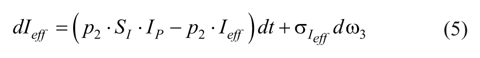
where
The glucose dynamics are described as,
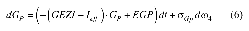
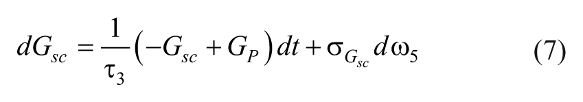
where
Identifiable Parameters in Medtronic Virtual Patient on SDE-GB Form.
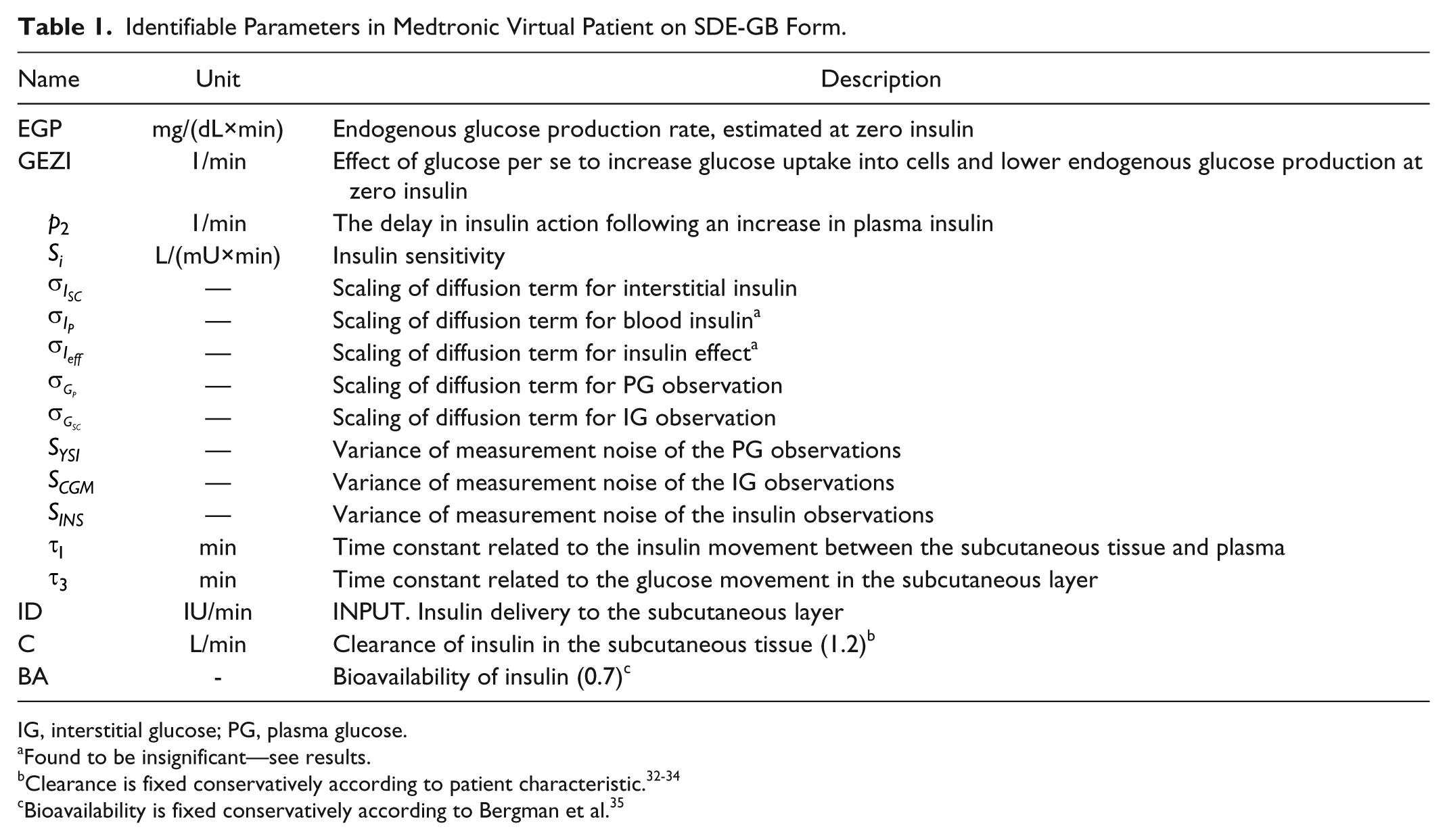
IG, interstitial glucose; PG, plasma glucose.
Found to be insignificant—see results.
Bioavailability is fixed conservatively according to Bergman et al. 35
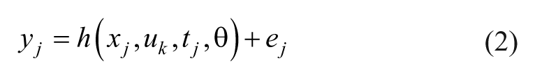
For our study the observation equations are,

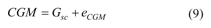
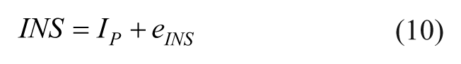
where
The Maximum Likelihood Principle
The likelihood function captures all the information in the data about the parameters. For time-series data, the likelihood function is a product of 1-step conditional densities. Due to the Gaussian increments of the Wiener processes, it is assumed that the conditional densities are Gaussian. To evaluate this, 1-step conditional predictions are needed. These are calculated using an extended Kalman filter,26,27 and the likelihood function has been identified as the key inferential quantity conveying all information in statistical modeling including uncertainty.32,39
Using the 1-step prediction error,
where
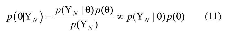
Assuming Gaussian distributions, the posterior probability density function becomes,
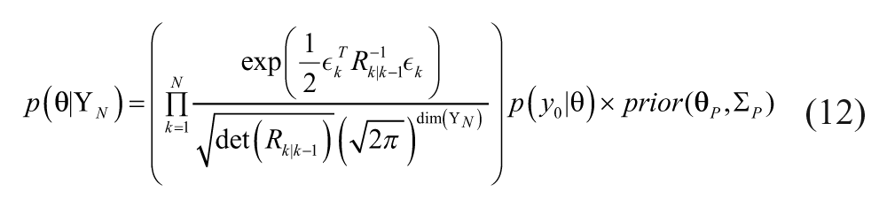
where
where
To mimic potential future applications, 3 different setups for the prior knowledge have been considered:
A theoretical prior knowledge for the variance of the measuring devices:
A prior knowledge formed by the estimate and covariance
A prior knowledge formed by the estimate and covariance
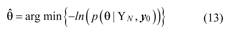
Modeling Process
All computations are performed using the statistical software R (version 2.15.1) and the CTSM-R package. 42 The identified models are cross-validated by analyzing the predictions from 2 study nights from the same patient. The following steps are followed for both data sets (see Table 2).
Flow of the Modeling Process.
IG, interstitial glucose; PG, plasma glucose.
All observations in the data set are used for estimation.
Only IG observations are used in the prediction of PG in this step.
Step 1 (Diffusion Term Identification and Maximum Likelihood)
In the initial model building process for diffusion step inclusion, forward selection and Likelihood ratio tests are used.26,27 (a) The parameters of the initial ordinary differential equation model,
Steps 2-6 (A Bayesian Method)
Step 2
For Data1 and Data2, each respective Bayesian estimate,
Step 3
With the estimates obtained in step 2, the predictions of PG for Data1 and Data2, are calculated using only the respective IG to verify the prediction capabilities.
Step 4
The new prior knowledge
Step 5
From Data1,
Step 6
With the obtained estimates
Results
For all estimates presented, identifiability has been established by testing different starting points of the estimation. The forward selection method gave statistical reason for diffusion term inclusion and resulted in the terms
Maximum Likelihood (Step 1)
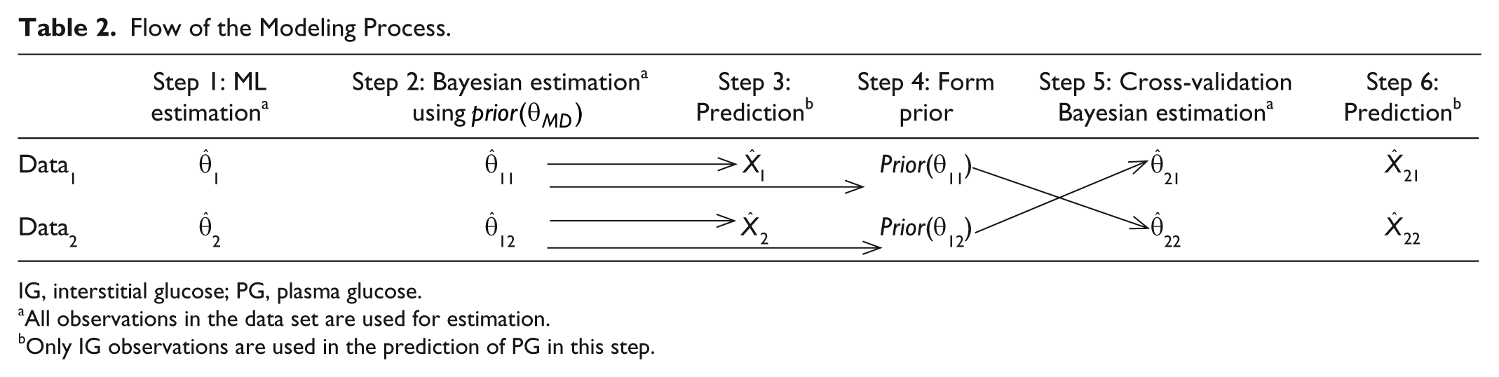
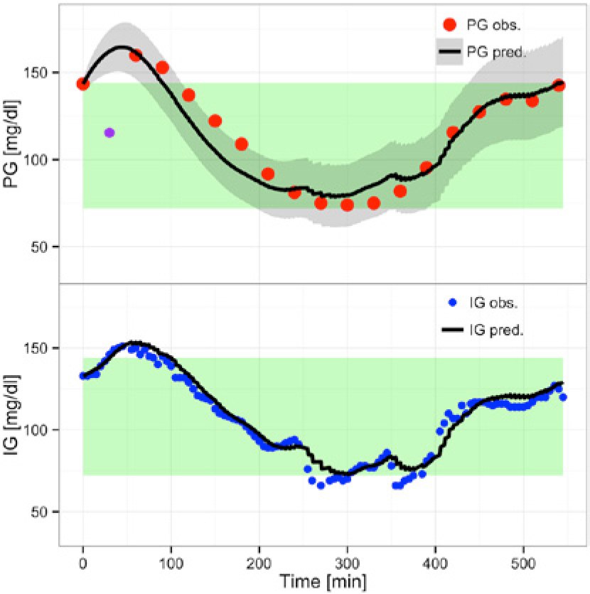
For the maximum likelihood investigation only the results from Data1 are presented. Results from Data2 show identical modeling behavior. Using CTSM-R, the 1-step-ahead prediction of PG and IG is obtained with calibration at each data point. As seen in Figure 1, the maximum likelihood estimate,
(Overall) Predicting with
It is evident that the overall prediction of PG follows the dynamic of the IG observations. Steep transitions in the prediction of PG are a direct result of a steep transition in IG observations. These transitions and the overall dynamic behavior are attributed to the maximum likelihood estimate, visualizing the challenge of the estimation technique. The parameter estimates are not presented, as the visual inspection shows suboptimal predictions. This is most easily seen by the persistent deviation between the predictions and the data over longer periods for the PG observations.
A Bayesian Method (Step 2)
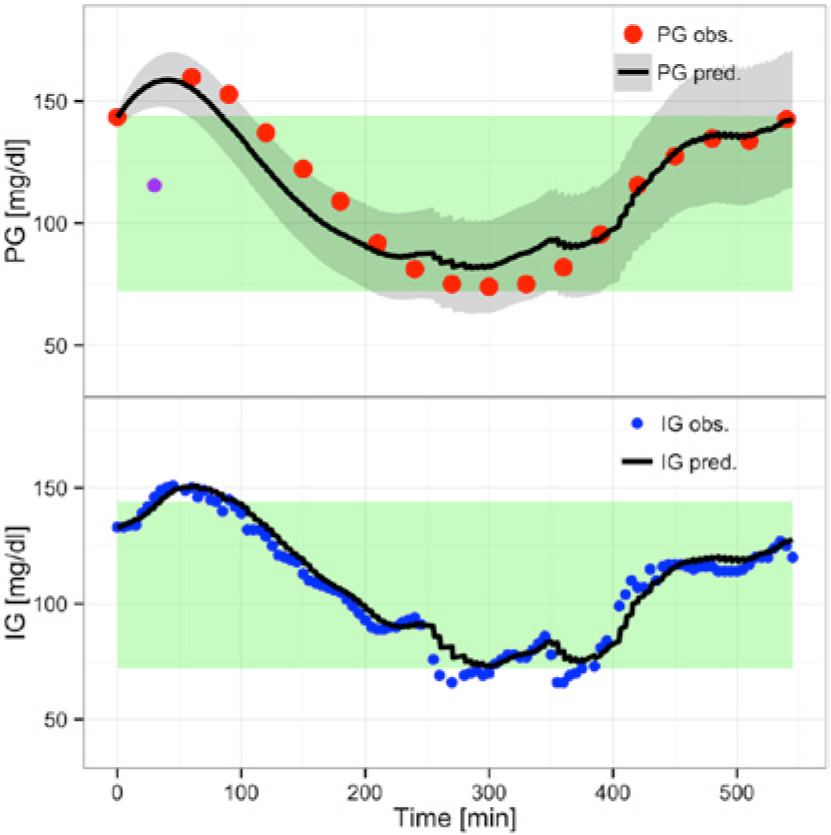
Figure 2 shows the predictions from a Bayesian estimation,
(Overall) Prediction with
The prediction of IG is not as precise as before and the confidence interval is wider, a direct consequence of the Bayesian method. The Bayesian method makes the prediction band for IG statistically meaningless. As we are interested only in the PG prediction, this is a minor problem. The IG prediction band will not be shown in the remaining results.
The prediction of PG is improved and the 95% prediction band is narrower. From a visual inspection it is seen that
It is not meaningful to statistically compare step 1 and step 2, as information criteria are defined from the pure likelihood function; therefore visual and physiological improvements are assessed.
Model Validation
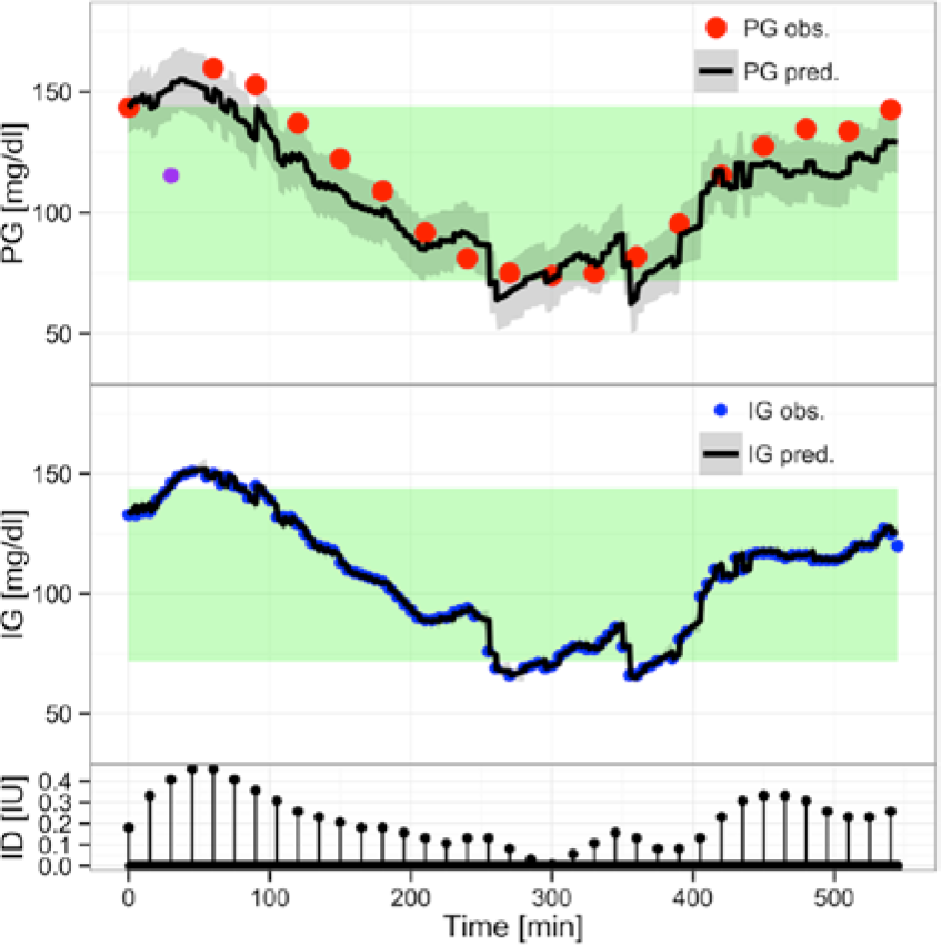
As it is desired to predict PG from IG observations, predictions without knowledge of the PG or insulin observations are computed.
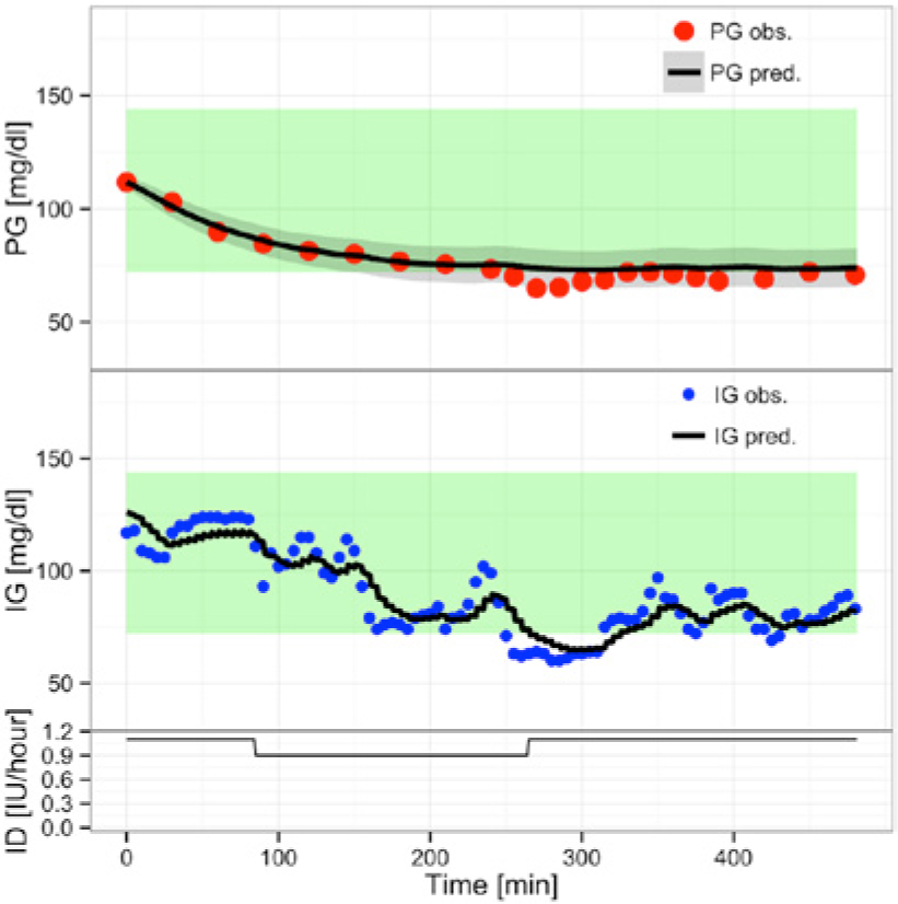
Data1
Prediction using
(step 3)
Figure 3 shows the 1-step-ahead prediction using
(Overall) Predicting with
Prediction using
(step 6)
Figure 4 shows the predictions using
(Overall) Prediction with
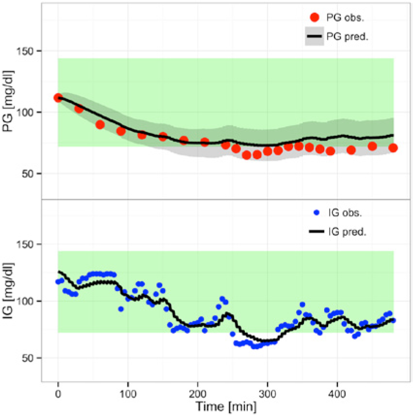
Data2
Predicting using
(Overall) Prediction with
Predicting using
(step 6)
Figure 6 shows the prediction using

(Overall) Prediction with
Discussion
This study shows that it is possible to predict PG from IG observations using a Bayesian method. This finding indicates that the final model can be used as a control algorithm that is implementable in a pump system.
Maximum Likelihood (Step 1)
Using maximum likelihood estimation, the IG influence on the PG prediction is evident. The many closely spaced observations have a tremendous influence on the likelihood. 32 The optimization minimizes the 1-step prediction, and as there are more IG observations, the optimizer will gain more from explaining the IG dynamics. To avoid this, a Bayesian method is suggested as a solution.
A Bayesian Method (Steps 2, 5 and 6)
It is assumed that the global parameter set for a patient will vary between days. This variation is assumed to have a limited span. This assumption enables us to cross-validate within the same patient. We expect that the parameter estimates from a given night will be similar to parameter estimates from another night. This allows us to use prior knowledge from 1 study night to estimate a new parameter set.
The ideal solution for a Bayesian method implementation is estimation of the optimal prior knowledge. However, an estimation of the variance of the variance of the measurement device requires a large amount of data. Instead, the literature was used to approximate measurement-device prior knowledge. The 95% prediction band is wide on the IG prediction since a Bayesian method is used. But as the focus of the study is prediction of PG this is accepted. The 95% prediction bands for PG are narrow.
As discussed by Donnet and Samson, Bayesian methods have been proposed and implemented for population pharmacokinetics/pharmacodynamics SDE-GB. 43 Using CTSM-R it is possible to implement Bayesian estimation on a single subject, obtaining valid and interpretable models. With this approach insulin observations are needed to estimate the parameters of the model. A similar approach could have been tested using clinical knowledge to fix the parameter. Future studies are needed to clarify this and should include several patients and preferably population modeling.
Physiological Modeling
The SDE-GB models applied allow for a physiological, opposed to a purely statistical, interpretation of the models, since the model structure is based on physiology. From a visual inspection it is evident that the statistical best model is not the physiologically and technologically most correct model.
The use of CTSM-R allows optimal conditions for the modeling procedure: that is, continuous-time dynamics with discrete time observations and a possibility of adopting a Bayesian modeling framework. This gives fewer parameters to estimate, which in turn gives a more robust estimation. Furthermore, previous knowledge is often given as differential equations, and therefore easily incorporated into existing models. 43 This maintains the physiological meaning of the model, and gives it interpretability for both the modelers and medical experts.
The examination of the covariance matrixes reveals that there is no severe parameter correlation. The covariance matrix has great potential in constructing a virtual patient database. Randomly selected parameter sets can be used to construct an infinite number of simulations for use as initial investigations, instead of costly human experiments.
Perspectives
A natural progression is to extend the Bayesian method to data where other factors, such as meals, have an influence. Building on Reifman et al., 16 a combination of data-driven AR models and Bayesian probability models should be investigated. The Bayesian probability ensures physiological interpretability and the AR processes capture sensor dynamics.
New optical-sensor techniques are currently under development as an alternative to the electrochemical transducer. Vaddiraju et al. provide an overview of advantages, disadvantages, and perspectives. 7
To obtain more knowledge about PG-IG dynamics, experiments with multiple glucose sensors, both electrochemical and optical, should be considered. Advantages of a multiple glucose sensor approach are not well investigated, but reports describing the advantages exist.44,45
Conclusion
The aim of this article was to extend an existing model describing PG-IG dynamical behavior to SDE-GB form With the SDE-GB model, and clinical data from a closed-loop study, parameters were estimated. The initial investigation used a maximum likelihood approach. Afterward a Bayesian method was investigated.
Using the maximum likelihood approach gave statistically reliable result, but there were deficiencies, as the ability to predict PG from IG observations was poor. A Bayesian method was successfully implemented, and it has been shown that parameters can be estimated using CTSM-R. Using a Bayesian estimate we were able to predict PG using IG observations. Furthermore we were able to cross-validate parameter estimates using a different data set from the same patient. Using prior knowledge from a previous study night, we were able to estimate usable parameters, indicating a close relation in intrapatient parameters.
These findings indicate that the model can be incorporated in an artificial pancreas that can be used as a closed-loop controller.
Footnotes
Appendix.
Estimated Parameter Values.
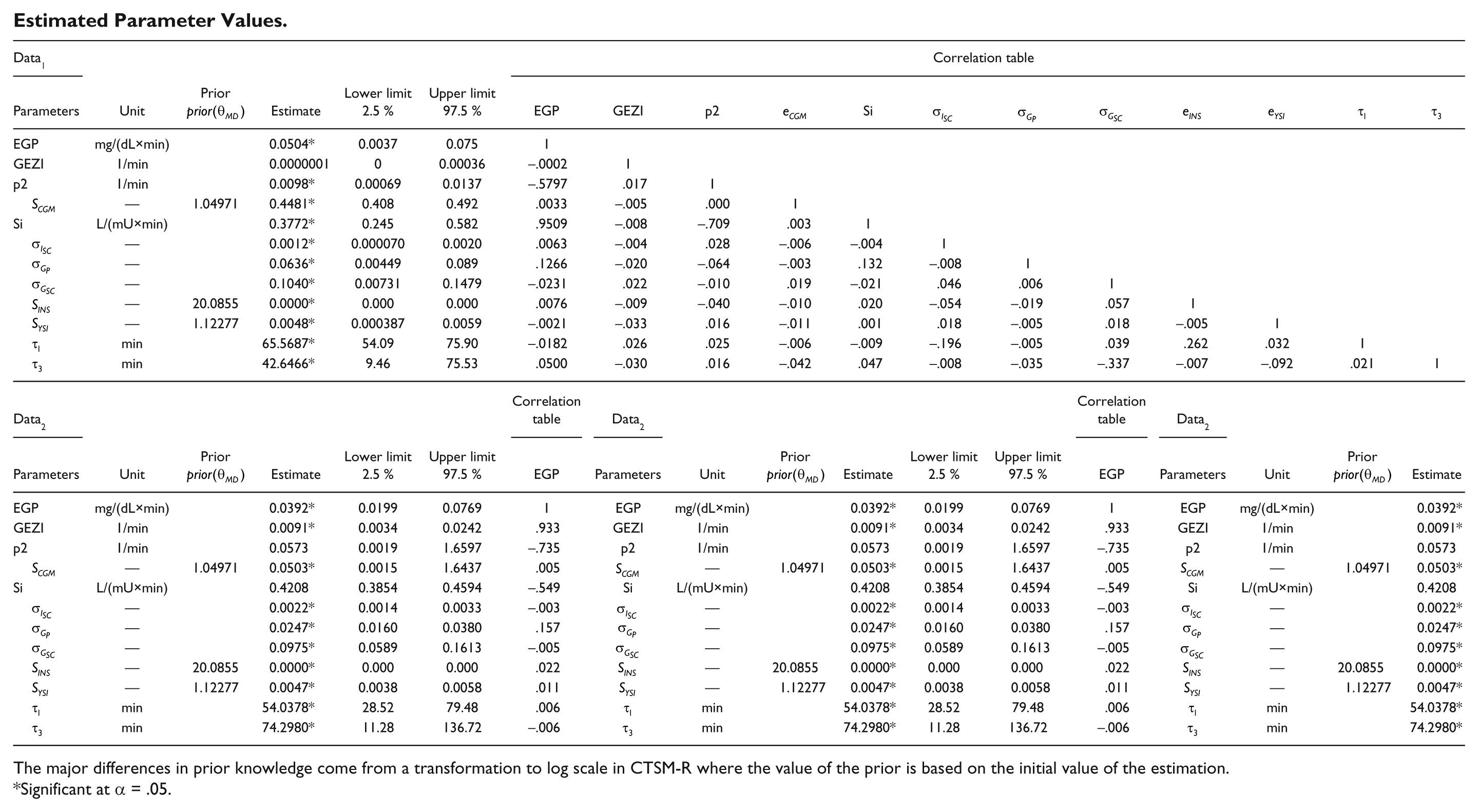
| Data1 |
Correlation table |
||||||||||||||||
|---|---|---|---|---|---|---|---|---|---|---|---|---|---|---|---|---|---|
| Parameters | Unit | Prior |
Estimate | Lower limit 2.5 % | Upper limit 97.5 % | EGP | GEZI | p2 |
|
Si |
|
|
|
|
|
|
|
| EGP | mg/(dL×min) | 0.0504* | 0.0037 | 0.075 | 1 | ||||||||||||
| GEZI | 1/min | 0.0000001 | 0 | 0.00036 | −.0002 | 1 | |||||||||||
| p2 | 1/min | 0.0098* | 0.00069 | 0.0137 | −.5797 | .017 | 1 | ||||||||||
| |
— | 1.04971 | 0.4481* | 0.408 | 0.492 | .0033 | −.005 | .000 | 1 | ||||||||
| Si | L/(mU×min) | 0.3772* | 0.245 | 0.582 | .9509 | −.008 | −.709 | .003 | 1 | ||||||||
| |
— | 0.0012* | 0.000070 | 0.0020 | .0063 | −.004 | .028 | −.006 | −.004 | 1 | |||||||
| |
— | 0.0636* | 0.00449 | 0.089 | .1266 | −.020 | −.064 | −.003 | .132 | −.008 | 1 | ||||||
| |
— | 0.1040* | 0.00731 | 0.1479 | −.0231 | .022 | −.010 | .019 | −.021 | .046 | .006 | 1 | |||||
| |
— | 20.0855 | 0.0000* | 0.000 | 0.000 | .0076 | −.009 | −.040 | −.010 | .020 | −.054 | −.019 | .057 | 1 | |||
| |
— | 1.12277 | 0.0048* | 0.000387 | 0.0059 | −.0021 | −.033 | .016 | −.011 | .001 | .018 | −.005 | .018 | −.005 | 1 | ||
| |
min | 65.5687* | 54.09 | 75.90 | −.0182 | .026 | .025 | −.006 | −.009 | −.196 | −.005 | .039 | .262 | .032 | 1 | ||
| |
min | 42.6466* | 9.46 | 75.53 | .0500 | −.030 | .016 | −.042 | .047 | −.008 | −.035 | −.337 | −.007 | −.092 | .021 | 1 | |
| Data2 |
Correlation table |
Data2 |
Correlation table |
Data2 |
|||||||||||||
| Parameters | Unit | Prior |
Estimate | Lower limit 2.5 % | Upper limit 97.5 % | EGP | Parameters | Unit | Prior |
Estimate | Lower limit 2.5 % | Upper limit 97.5 % | EGP | Parameters | Unit | Prior |
Estimate |
| EGP | mg/(dL×min) | 0.0392* | 0.0199 | 0.0769 | 1 | EGP | mg/(dL×min) | 0.0392* | 0.0199 | 0.0769 | 1 | EGP | mg/(dL×min) | 0.0392* | |||
| GEZI | 1/min | 0.0091* | 0.0034 | 0.0242 | .933 | GEZI | 1/min | 0.0091* | 0.0034 | 0.0242 | .933 | GEZI | 1/min | 0.0091* | |||
| p2 | 1/min | 0.0573 | 0.0019 | 1.6597 | −.735 | p2 | 1/min | 0.0573 | 0.0019 | 1.6597 | −.735 | p2 | 1/min | 0.0573 | |||
| |
— | 1.04971 | 0.0503* | 0.0015 | 1.6437 | .005 |
|
— | 1.04971 | 0.0503* | 0.0015 | 1.6437 | .005 |
|
— | 1.04971 | 0.0503* |
| Si | L/(mU×min) | 0.4208 | 0.3854 | 0.4594 | −.549 | Si | L/(mU×min) | 0.4208 | 0.3854 | 0.4594 | −.549 | Si | L/(mU×min) | 0.4208 | |||
| |
— | 0.0022* | 0.0014 | 0.0033 | −.003 |
|
— | 0.0022* | 0.0014 | 0.0033 | −.003 |
|
— | 0.0022* | |||
| |
— | 0.0247* | 0.0160 | 0.0380 | .157 |
|
— | 0.0247* | 0.0160 | 0.0380 | .157 |
|
— | 0.0247* | |||
| |
— | 0.0975* | 0.0589 | 0.1613 | −.005 |
|
— | 0.0975* | 0.0589 | 0.1613 | −.005 |
|
— | 0.0975* | |||
| |
— | 20.0855 | 0.0000* | 0.000 | 0.000 | .022 |
|
— | 20.0855 | 0.0000* | 0.000 | 0.000 | .022 |
|
— | 20.0855 | 0.0000* |
| |
— | 1.12277 | 0.0047* | 0.0038 | 0.0058 | .011 |
|
— | 1.12277 | 0.0047* | 0.0038 | 0.0058 | .011 |
|
— | 1.12277 | 0.0047* |
| |
min | 54.0378* | 28.52 | 79.48 | .006 |
|
min | 54.0378* | 28.52 | 79.48 | .006 |
|
min | 54.0378* | |||
| |
min | 74.2980* | 11.28 | 136.72 | −.006 |
|
min | 74.2980* | 11.28 | 136.72 | −.006 |
|
min | 74.2980* | |||
The major differences in prior knowledge come from a transformation to log scale in CTSM-R where the value of the prior is based on the initial value of the estimation.
Significant at α = .05.
Abbreviations
CGM, continuous glucose monitor; CSII, continuous subcutaneous insulin infusion; IG, interstitial glucose; MVP, Medtronic virtual patient; PG, plasma glucose; SDE-GB, stochastic-differential-equation-based gray-box; SDEs, stochastic differential equations; T1DM, type 1 diabetes mellitus.
Declaration of Conflicting Interests
The author(s) declared no potential conflicts of interest with respect to the research, authorship, and/or publication of this article.
Funding
The author(s) disclosed receipt of the following financial support for the research, authorship, and/or publication of this article: This work was funded as a part of the DIACON project by the Danish Council of Strategic Research (NABIIT project 2106-07-0034).